Abstract
A testing method is developed to evaluate the acceleration- and strain-based fatigue life of a thermal interface layer in the high-cycle fatigue regime. The methodology adopts vibration-based fatigue testing, where adhesively bonded beams are excited at their resonant frequency under variable amplitude loading using an electrodynamic shaker. Fatigue failure is monitored through shifts in modal frequency and modal damping. Key findings include the identification of a 4% frequency shift as the failure criterion, corresponding to macro-delamination. The thickness of the thermal interface material influences acceleration-based fatigue life, decreasing by a factor of 0.2 when reduced from 0.3 mm to 0.15 mm and increasing by 5.5 when increased to 0.5 mm. Surface quality has a significant impact on both acceleration-based and strain-based fatigue curves. Beams from chemically etched aluminum–magnesium alloy specimens exhibit a sevenfold increase in fatigue life compared to beams from untreated printed circuit boards. Strain-based fatigue life increases with temperature, with a 0.2 reduction at °C and an eightfold increase at °C relative to °C. The first principal strain is validated as a reliable local damage parameter, effectively characterizing fatigue behavior across varying TIM thicknesses.
1. Introduction
In the wake of the current technology trends of electrified power trains and connected as well as autonomous driving, the level of integration and miniaturization of automotive electronics is notably increasing. Correspondingly, adequate thermal management is necessary in order to ensure optimal operating conditions for high-power density electronics. This is typically achieved through thermally conductive gap fillers, usually referred to as thermal interface materials (TIMs), which connect printed circuit boards (PCB) and/or electronic components to a heat sink and therefore improve their heat dissipation efficiency. In addition to this main function, the TIMs are known to positively impact the dynamic behavior of automotive electronic systems as a result of the established adhesive connection together with their relatively high structural damping [1,2].
Hence, it is crucial to study the degradation effects of TIMs in order to ensure the reliability and safety of automotive electronics under operating loading conditions. The former can be classified into climatic and dynamic loads. Since the climatic loads including humidity, thermal loads and thermal–mechanical loads appear to be the major cause of failure in automotive electronics, most of the research work on the reliability of TIMs addressed the failure mechanisms and fatigue life prediction under the above-mentioned loads [3,4,5]. However, during their manufacturing process, shipping and through their service life, automotive electronics involving TIMs are subjected to broadband dynamic loads stemming from road bumps and engine compartment oscillations. The knowledge of the high-cycle fatigue (HCF) properties of TIMs is therefore mandatory for the design of reliable automotive electronic systems.
In this regard, the current investigation aims at characterizing the HCF performance of a TIM applied in engine control units (ECUs) as an adhesive gap filler attaching PCB to housing in order to improve the thermal management of ECUs. A growing interest is directed toward understanding the effect of adhesive fatigue failure of the TIM on the lifetime of electronic components in ECUs, which are typically designed to meet a failure-free criterion over an extended operational life typically exceeding the threshold of stress cycles.
Experimental procedures for characterizing the HCF performance of materials and specimens can be broadly classified into two main approaches: non-resonant and resonant techniques. Non-resonant testing methods predominantly use servo-hydraulic fatigue testing machines, which typically operate at excitation frequencies below 20–50 Hz [6]. Although these conventional machines are widely used for low-cycle fatigue (LCF) testing [7,8], their application for reaching stress cycles in the HCF regime remains challenging due to several factors. These include significant energy consumption caused by the continuous generation of oil pressure for each cycle [6], prolonged testing times that can extend up to several weeks to reach cycles [9] and inherent fatigue of the testing apparatus, which makes damage monitoring difficult due to potential strain gauge failures [10].
The resonant techniques make use of a mechanically or electromagnetically induced oscillator to drive a machine/specimen combination into a resonant or near-resonant condition. As a result, these machines enable higher testing frequencies while maintaining lower power consumption. A concise historical overview of resonant testing techniques over the past century is provided by [11]. Nowadays, the interest in the usage of electrodynamic shaker testing facilities to study the fatigue of suitably designed resonant specimens is on the rise. Depending on the design of the tested specimen, high excitation amplitudes can be reached in the specimen’s resonant frequency range. A valuable contribution to the shaker-based resonant HCF testing was introduced by George et al. [11,12]. The authors designed a plate specimen which was base-excited through sine wave-forms using an electrodynamic shaker and driven into a high-frequency resonant mode. Due to the shift in the natural frequency of the tested specimen, the authors had to interrupt the test many times to manually adjust the excitation frequency to meet the new peak response and continue the fatigue process [11]. An enhancement to the latter work is proposed by [13], who managed to design an uninterrupted fatigue test consisting of a sinusoidal excitation of the test structure at a constant frequency from the near-resonant area by recurring a real-time phase-locked control loop. The authors failed, however, to excite the specimen at exactly its resonant frequency. This led to the loss of more than one-third of the resonance amplification. In [14], the authors designed a fatigue test for cantilever plates and managed to produce a constant amplitude sinusoidal excitation at the specimens’ fundamental frequency. Although the shift in the modal frequency allowed the authors to detect the damage initiation, it led to a drastic reduction in the induced strain amplitude in the specimen since the excitation frequency was not continuously adjusted during the test to match the fundamental frequency. As a consequence, this test methodology yields a very long testing duration in case larger-scale damage of the specimen is targeted, e.g., when studying the crack propagation or characterizing the total failure. In a more recent study by [15], the authors introduced a shaker-based fatigue test and successfully reached cycle numbers within the very high cycle fatigue (VHCF) regime for a thin-walled structure. However, they were unable to excite the specimen precisely at its resonant frequency. Similar to the findings in [13], this limitation resulted in reduced testing efficiency and prolonged test durations.
Examples of HCF tests on adhesive assemblies using electrodynamic shakers include those introduced in [16,17,18]. In [16], the authors designed a fatigue test for single lap joints, employing sinusoidal signals to excite the specimens at their fundamental frequency. In the work of [17,18], a new HCF test method for adhesive assemblies was presented. The specimens consisted of a ceramic component bonded to a printed circuit board (PCB) and were designed to simulate real-world service conditions. Through an in-house control routine, the deflection amplitude was kept constant all along the test, and the excitation frequency was continuously adjusted to exactly meet the specimen’s fundamental frequency. Although different vibrational parameters such as the frequency f, the phase lag , the maximal deflection Z and the local strain were monitored through the fatigue process, the authors faced difficulties in the definition of a failure criterion for the bi-axial specimen based on the time behavior of the measured signals.
To summarize, the aforementioned contributions suggest promising shaker-based HCF testing methodologies, of which the substantial advantage resides in saving time and power consumption by making use of the resonance effects of the tested specimens. In all of these works, a sinusoidal excitation signal was used at a constant frequency and amplitude. This urged unavoidable challenges such as the need for sophisticated control routines to track the resonance and make use of the local amplification effects during the test as well as the difficulties in monitoring modal parameters and detecting the exact time at which the failure is occurring. Another substantial limitation is that automotive electronic systems are subjected to random vibration variable amplitude (VA) loads stemming from road irregularities. Therefore, relying on fatigue data from constant amplitude tests to assess fatigue life under variable amplitude service loads can be misleading [19,20].
These observations motivate the current study, which aims at characterizing the fatigue performance of a TIM from automotive electronic applications in the HCF regime. For this sake, purposely designed adhesive assemblies are base-excited using an electrodynamic shaker and driven into oscillations at their fundamental frequency. To overcome the above difficulties, a VA excitation signal is proposed consisting of a white noise load collective at a user-defined frequency range. By adequately choosing the frequency range of the VA signal, an uninterrupted excitation of the resonant frequency of the specimen is guaranteed throughout the fatigue test without recurring to adjust the excitation signal’s parameters. This significantly simplifies the online monitoring of transmissibilities at frequent intervals, thereby enhancing the accuracy in evaluating the shift in modal parameters throughout the test period. A failure criterion is then defined based on the correlation of the shift in the modal parameters to the damage, i.e., the interface delamination length and the fatigue curves are established for the TIM under study. Another key novelty of this study is the testing of specimens with varying interface layer thicknesses, ranging from 0.15 mm to 0.5 mm, under different temperature conditions. This approach enables a comprehensive analysis of the effects of climatic and geometric parameters on the fatigue performance of the tested adhesive assemblies. The following section provides a brief survey of the influence of these parameters on the fatigue performance of adhesive joints.
Several studies have investigated the influence of bondline thickness on the fatigue performance of adhesive joints, yielding varying conclusions. Comprehensive reviews on this topic are provided by [21,22]. Experimental findings from multiple studies [23,24,25] suggest the existence of an optimal bondline thickness, beyond which the fatigue performance of structural adhesive joints deteriorates. This decline is often attributed to an increased likelihood of defects, micro-cracks and voids within the adhesive layer, which facilitate premature fatigue crack initiation [22]. Conversely, a number of studies report an improvement in the fatigue performance of bonded joints with increasing adhesive thickness. For instance, ref. [26] observed this effect in elastomeric silicone adhesive joints, while [16] demonstrated a significant enhancement in the fatigue strength of single-lap joints with an increased adhesive thickness in the frontal area of the joint.
The effect of temperature on the fatigue performance of adhesive joints primarily depends on the adhesive material. A key factor influencing this behavior is the glass transition temperature () of the adhesive. Below , the adhesive behaves as a low-strain, rigid material, whereas above this temperature, it becomes more flexible with rubber-like properties. Common epoxy adhesives typically have a above room temperature, while flexible silicone adhesives typically undergo glass transition below −100 °C. Since mechanical properties change significantly when this transition occurs, experimental studies on epoxy-based structural adhesive joints consistently report a decline in fatigue strength with increasing temperature [27,28,29]. One of the few studies investigating the effect of temperature on elastomeric silicone adhesives is presented in [26]. Their research examined two different silicone adhesives, revealing contrasting behaviors: while the lap-shear strength of one adhesive decreased with increasing temperature, the other exhibited an opposite trend.
To the authors’ best knowledge, the impact of the above parameters on the high-cycle fatigue performance of a silicone-based thermal interface layer under random vibration loads is investigated for the first time in this study. The remainder of this paper is outlined as follows: Section 2 details the fatigue testing methodology, beginning with an overview of the studied material and its relevant properties, followed by a description of the specimens, test setup and experimental procedure. The damage identification method based on shifts in modal parameters is then introduced, along with the failure criterion for the tested assemblies. Furthermore, the numerical procedure used to evaluate local TIM strains is presented. Section 3 discusses the main findings, including the derivation of the fatigue curves (- and -) and a parametric analysis assessing the effects of TIM thickness, surface quality and temperature on the fatigue performance of the tested assemblies.
2. Materials and Methods
This section describes the investigated material, tested specimens, test setup, damage identification method and numerical procedure.
2.1. Material Characterization
The studied material is a two-component soft silicone filled with aluminum oxide (A) particles, which is widely used as a thermally conductive adhesive gap filler in automotive electronic systems. Its primary function is to dissipate heat from PCBs and electronic components by conducting it to a heat sink, such as aluminum housing. In [1], a numeric–experimental identification methodology of the dynamic material properties of the TIM under study was proposed and validated. The main output of this study was the characterization of the frequency- and temperature-dependent complex shear modulus of the TIM and the curve fitting to a fractional derivative viscoelastic material model [30]. The complex shear modulus is defined as
, and denote the frequency-dependent storage modulus, loss modulus and loss factor, respectively. The loss factor is a measure of the energy dissipated per cycle relative to the stored energy in a vibrating system and is related to the damping ratio by
The fractional derivative form of the complex modulus is given by
where and represent the relaxation modulus and glassy modulus, respectively, while and are the fractional parameters. The identified fractional derivative parameters at 20 °C are listed in Table 1.

Table 1.
Parameters of the fractional derivative model of the complex shear modulus at 20 °C.
The curves of the frequency-dependent complex modulus at different temperatures are obtained through the temperature-dependent horizontal and vertical shift factors ( and ), as shown in Table 2. These factors are defined by
Table 2.
Horizontal and vertical shift factors and for obtaining the shear modulus at −40 °C and 100 °C from the reference curve at 20 °C.
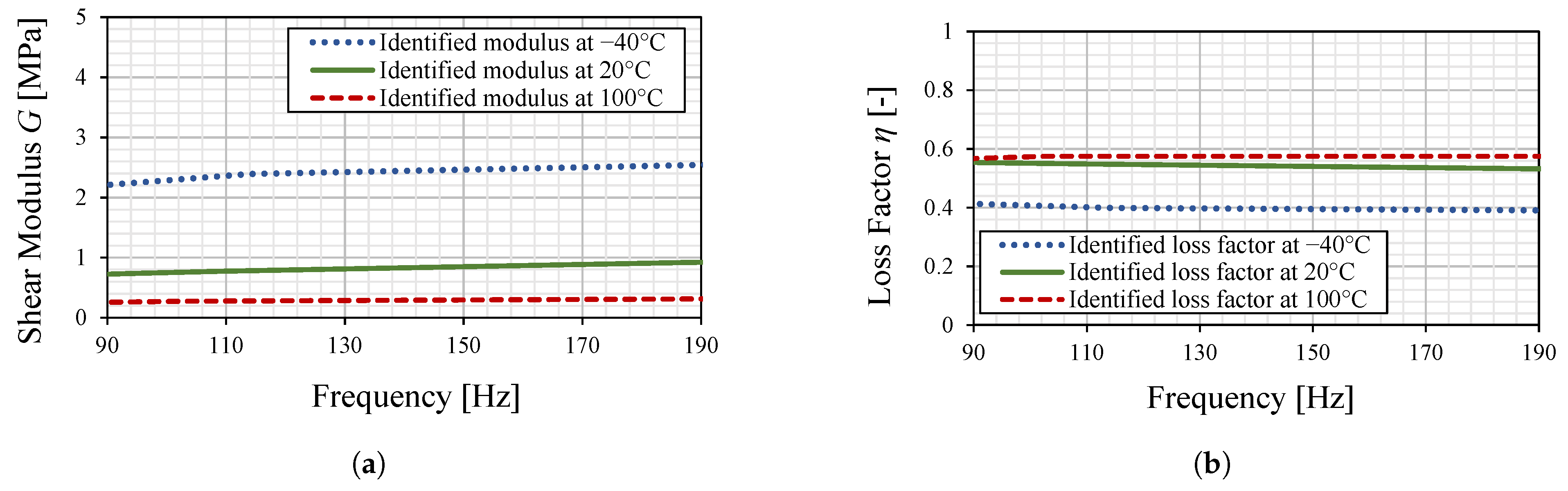
In the current study, the experiments are conducted at frequencies in the vicinity of the first bending mode of the tested specimens. Taking into account the shift in the main resonance throughout the tests as well as the scattering of the different specimens, the relevant frequency range can be reduced to 90–190 Hz. Figure 1 illustrates the evolution of the shear modulus and loss factor in the above frequency range.
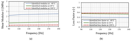
Figure 1.
Identified shear modulus (a) and loss factor (b) of the TIM under study in the frequency range of the conducted HCF experiments in this study.
Notably, the material parameters exhibit a flat behavior, indicating that the stiffness loss due to the frequency dependence of the dynamic material properties is negligible in this range.
Table 3 provides an overview of the material parameters of the TIM for the relevant temperatures considered in this study. The Poisson’s ratio is assumed to be constant across the tested temperatures, as it generally exhibits a flat behavior above the glass transition temperature. For the material under study, this transition occurs at approximately −100 °C, justifying the use of a constant value in the analysis [31].
Table 3.
Overview of the materials parameters of the TIM at relevant temperatures.
2.2. Geometry and Test Setup
The test structure consists of beam structures bonded to an aluminum plate using an adhesive thermal interface layer. Two different beam materials are evaluated in this study: AlMg3 and FR4 PCB. AlMg3, also known as EN AW-5754, is a non-heat-treatable aluminum–magnesium alloy containing approximately 3% magnesium by weight. FR4 is a composite substrate material consisting of alternating layers of fiberglass-reinforced epoxy resin and conductive copper. The tested PCB beams feature a four-layer copper structure and are coated with a green, photoimageable solder mask (PROPIMER® 77).
The TIM is applied with uniform thickness over the overlap area, ensuring consistency and precision using auxiliary spacers and dispensing forms. To further minimize scatter in dynamic behavior and therefore enhance the robustness of the identified fatigue model, tight machining tolerances are applied to the aluminum beams. The TIM is then cured for 30 min at 50 °C, ensuring optimal mechanical performance and bonding integrity.
One substantial advantage of the presented geometry is the ability to test up to six beams in one test run. In addition to the reproducibility and statistical robustness, the required testing time to identify the HCF limit is clearly reduced. The adopted test structure is illustrated in Figure 2 while the geometrical parameters and the different combinations of the tested specimens are summarized in Table 4.
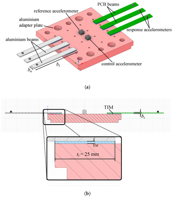
Figure 2.
Three-dimensional (a) and zoom-in (b) views of the adopted test structure: Six beams are adhesively assembled to an aluminum adapter plate mounted on an electrodynamic shaker. Both beam material and TIM thickness (w) are varied within the scope of an HCF parametric study.
Table 4.
Geometry and material parameters of the beam structures.
The test structure is then mounted on the rigid base plate of an electrodynamic shaker to perform the vibration tests as illustrated in Figure 3.

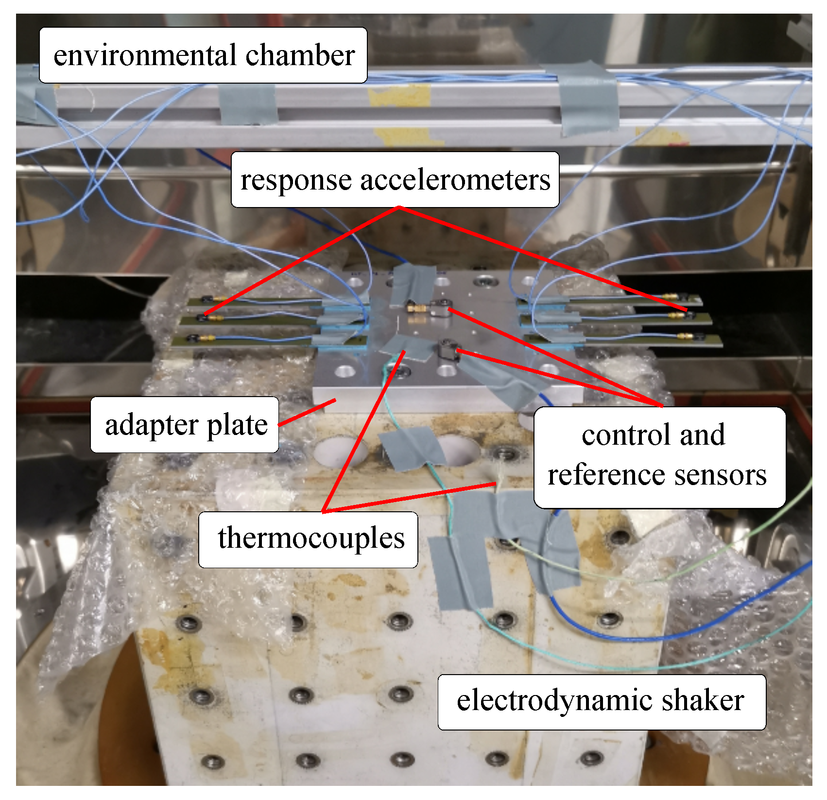
Figure 3.
Shaker test setup: B02 specimens mounted on the rigid shaker base inside an environmental chamber.
The shaker is placed inside an environmental chamber allowing HCF tests under different temperature conditions while thermocouples are applied in order to monitor the chamber and specimens’ temperature throughout the tests. Three constant temperatures are chosen for the fatigue tests of the specimens B02: room temperature (23 °C), low temperature (−40 °C) and high-temperature conditions (100 °C). All of the other specimen variants are tested under room temperature conditions (23 °C). The lower temperature limit of −40 °C was selected to prevent entering the crystallization range of the silicone-based TIM, which begins around −50 °C and leads to abrupt changes in dynamic material properties, causing measurement uncertainties.
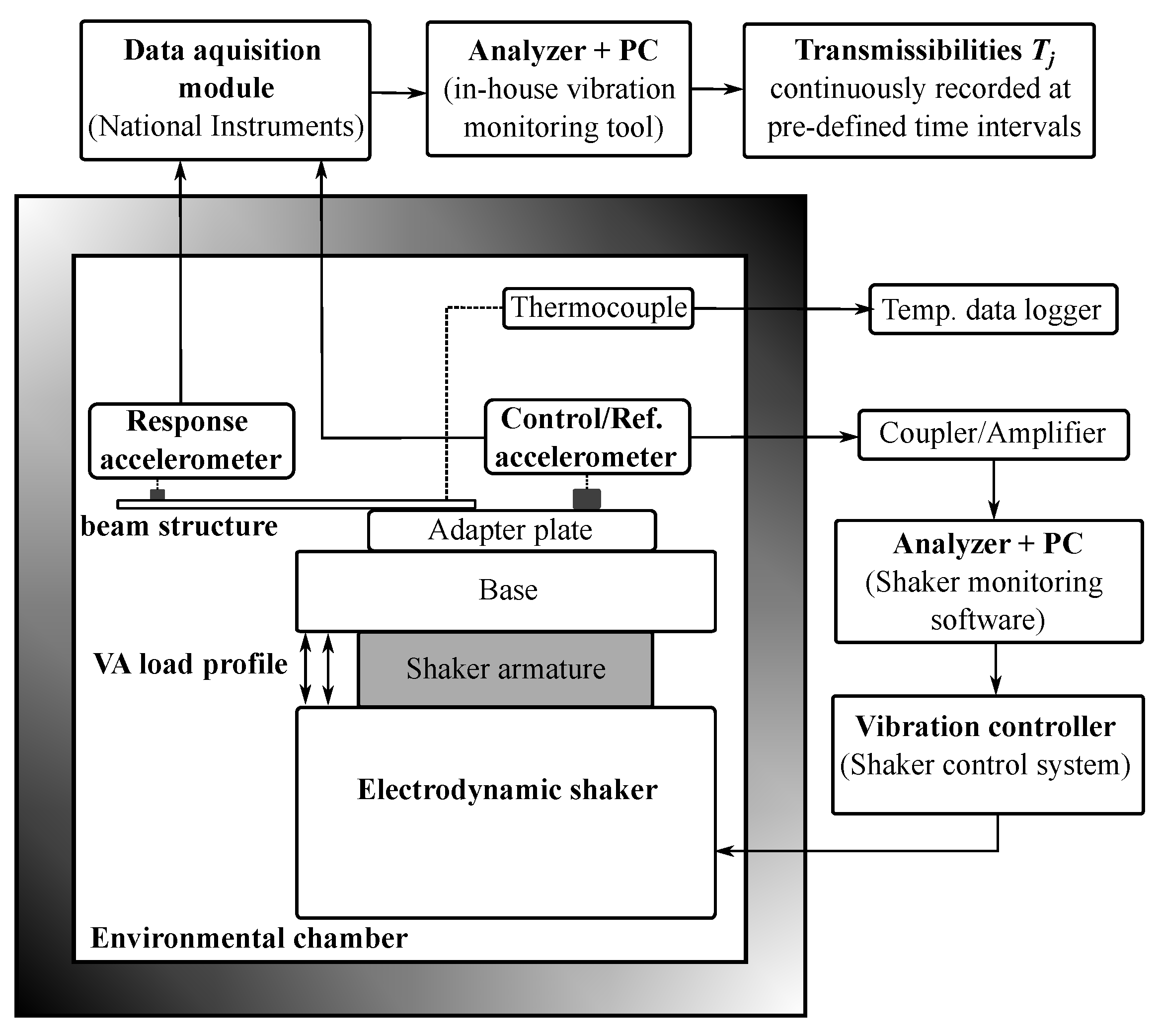
The acceleration of the shaker is measured and controlled by a piezoelectric accelerometer mounted on the adapter plate. In order to establish the transmissibility function corresponding to the acceleration input–output ratio, lightweight accelerometers (0.2 g) are placed toward the free end of the beams to measure the transverse acceleration response. Although these low-mass sensors minimize disturbances in the measured transmissibility, they have limitations in their operational temperature range. Specifically, their characteristic curve deviates from a flat response as temperatures approach 100 °C. Furthermore, the performance of the adhesive used to mount them on the beams degrades above 100 °C. These constraints influenced the selection of the upper temperature limit in this study. A schematic block-diagram of the experimental procedure is illustrated in Figure 4.

Figure 4.
Block-diagram of the experimental setup of the conducted HCF tests.
2.3. Experimental Procedure
The experiments are conducted on each of the specimens A0x and B0x as in Table 4 following the sequence presented in Figure 5. First, a resonance measurement at a low excitation level is performed with the main target of identifying the frequency range of the first transversal bending mode of the beams. The low excitation level guarantees avoiding undesirable pre-damages to the adhesive TIM layer. Examples of the measured transmissibilities of the first transverse mode are plotted in Figure 6.
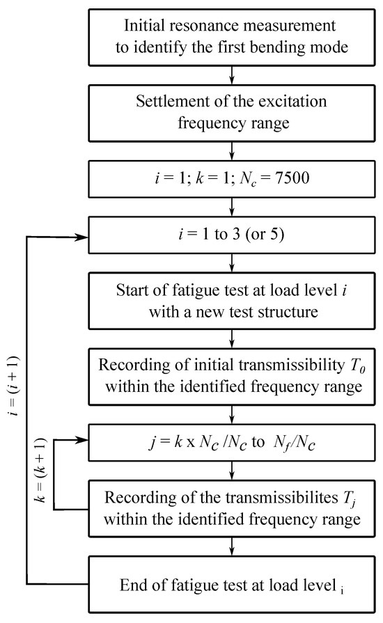
Figure 5.
Test sequence of the conducted HCF investigations for each specimens’ variant: A0x and B0x.

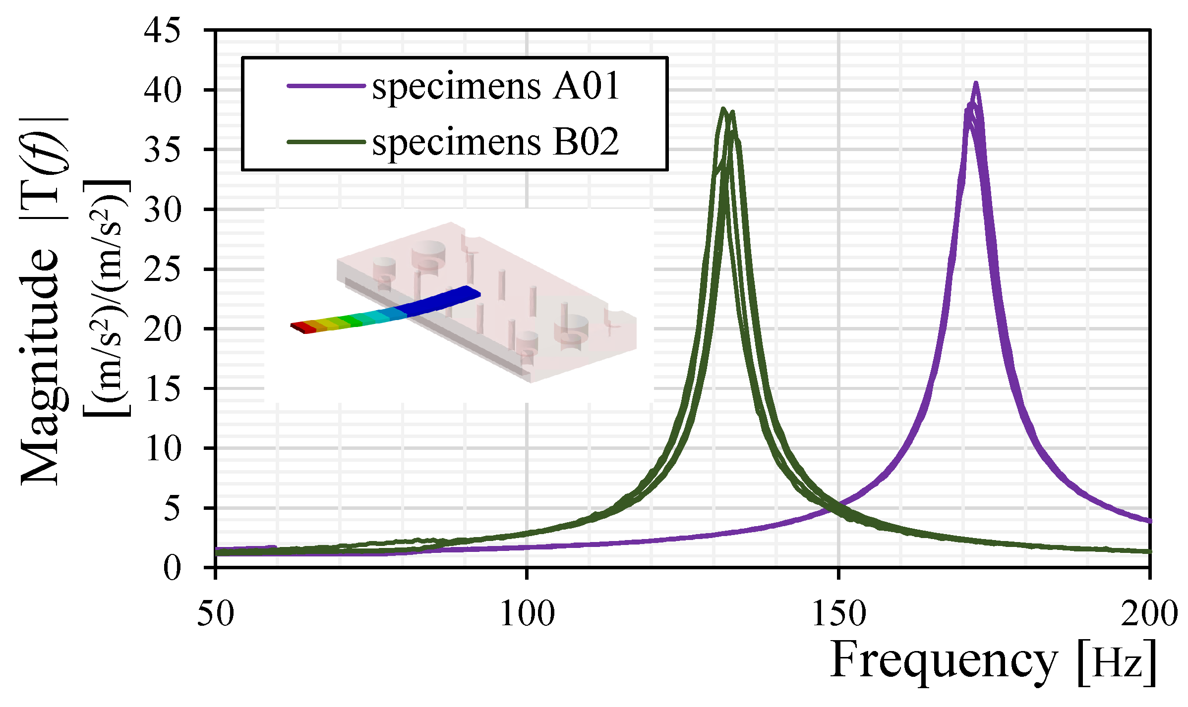
Figure 6.
Transfer functions of the specimens A01 and B02 established in the initial resonance measurement in order to identify the relevant frequency range for the fatigue tests.
A comparison between the measured and the theoretical natural frequencies of these beams is presented in Table 5. The analytical solution is calculated according to Bernoulli beam theory [32] for a cantilever beam with a single lap joint and is given by
where is the first mode shape coefficient, E is Young’s modulus (Pa), I is the moment of inertia (), is the material density () and A is the cross-sectional area (). The effective beam length is defined as [33]
where L is the total beam length, is the lap joint length and is the stiffness reduction factor, which varies between 0.5 and 1, depending on the joint properties. A higher value is typically observed in flexible adhesive joints and when the beams are made of different materials, as these conditions introduce additional compliance and reduce the overall stiffness of the structure [33]. As the resonant frequency is mainly determined by the beam’s elastic properties and boundary conditions, the adhesive layer influences it indirectly by modifying the effective free length as damage progresses. Crack initiation and propagation in the TIM layer reduce joint stiffness, leading to a gradual frequency shift. This effect is particularly relevant for tracking fatigue-induced degradation, as changes in resonance behavior correlate with interface weakening and delamination growth.
Table 5.
Comparison of analytically and experimentally identified natural frequencies of the first transversal mode of the tested beam structures.
In Figure 6, the PCB specimens exhibit greater scatter in the measured resonance compared to the aluminum ones. This is primarily due to the tighter machining tolerances applied to the aluminum beams, whereas the PCB beams were cut with less precision. Additionally, the multi-layer structure of the PCB introduces thickness scattering and equivalent elastic modulus variation due to material inconsistencies and fabrication tolerances.
Two different excitation frequency ranges for the aluminum and the PCB beams, yet with the same width, are opted for in the fatigue test, namely [20 Hz–200 Hz] for the PCB beams and [60 Hz–240 Hz] for the aluminum beams. The chosen bandwidth ensures that both specimen types, A0x and B0x, experience the same effective acceleration load () while also accounting for differences in their average first modal frequency. Moreover, it accommodates the progressive shift in the first modal frequency to lower values during the fatigue test, as revealed later in Figure 8a, ensuring continuous excitation of the first mode throughout the test until total delamination.
The choice of the bandwidth as well as of the appropriate load level for the fatigue test is based on the results of a precedently performed step-stress test (SST) for the chosen specimen’s variants. The SST consists of continuously increasing the shaker load amplitude at constant time steps while keeping the frequency range constant until failure occurs. By doing so, both the required load level as well as the time to failure for the actual fatigue test are rapidly estimated.
In order to monitor changes in the transfer behavior of the beam structures, the transmissibility functions (, ) are continuously recorded throughout the tests every 60 s, which roughly corresponds to an average number of cycles of = 7500 as mentioned in Figure 4. This automated monitoring procedure allows for the detection of changes in the modal parameters corresponding to stiffness loss and establishing a failure criterion for the adhesive TIM layer. The fatigue test at each load level is terminated once all beams experience complete delamination, resulting in their detachment from the base plate, or when the threshold of cycles is approached for the lowest load levels. The number of cycles completed by the tested specimens upon meeting these termination criteria is denoted as in Figure 5.
For both SST and actual fatigue tests, a VA base excitation consisting of a white noise acceleration spectral density (ASD) profile is chosen. The choice of VA loads in the current investigation rests on the following arguments:
- –
- As previously stated, the bandwidth of the testing profile allows for a continuous excitation of the main beam transversal mode and an uninterrupted monitoring of the modal parameters throughout the test without resorting to sophisticated control loops to adjust the frequency range along the test.
- –
- Since the fatigue behavior can be highly sensitive to the load time history, the classic approach of performing laboratory tests under constant amplitude (CA) load conditions to predict the lifetime under VA service loads may lead to inconsistencies and a lack of validity. Major reasons for this observation are potential differences in damage initiation sites, mechanisms of damage growth as well as threshold effects when cycles with high loads are mixed with small amplitude, but more frequent, load cycles [20].
- –
- The valuable contribution of E. Gaßner who performed VA fatigue experiments as early as in the 1940s is taken into account [34,35]. Based on these experiments, he then introduced the “scale lines”, which are nowadays called “Gaßner-curves”, where he plotted the fatigue life as a function of the maximum loads from the applied excitation load collectives [36].
Figure 7a illustrates an example time signal generated for a chosen load level from the fatigue test: AS = 4 (m//Hz, as in Figure 7c. The corresponding rainflow matrix histogram is displayed in Figure 7b. Indeed, the excitation signal can be divided into distinct load sequences with different amplitudes and frequencies of occurrence contributing each to the fatigue process of the TIM under study. An overview of the shaker excitation profile parameters at the different load levels from the fatigue tests of the specimen B02 is summed up in Table 6.
Table 6.
Overview of the shaker excitation profile parameters for the specimen B02 during the fatigue test.
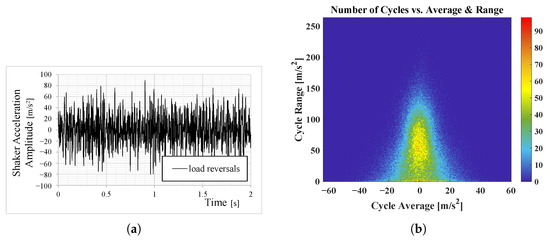

Figure 7.
Example of time-series signal (a) and 2D rainflow matrix histogram [37] (b) for the shaker excitation profile at a chosen load level from the fatigue test (ASD = 4 (m//Hz) (c).
Figure 7.
Example of time-series signal (a) and 2D rainflow matrix histogram [37] (b) for the shaker excitation profile at a chosen load level from the fatigue test (ASD = 4 (m//Hz) (c).


2.4. Damage Identification Based on Modal Parameters
As already pointed out, the transmissibilities are monitored along the fatigue test at each of the corresponding load levels, in order to detect possible changes in the transfer behavior, i.e., in the modal parameters of the tested beam structures.
In fact, the interest in relying on the modal parameters to detect damage in structures is on the rise. This is mainly due to the fact that the structural modal parameters (natural frequencies, mode shape and modal damping) are functions of the physical properties of the inspected structure. Therefore, changes in the latter parameters can be taken as proof of the existence, location and severity of structural damages. Extensive reviews of modal-based damage identification methods are given by [38,39]. These works mainly focused on surveying damage identification methods which use either modal frequency or mode shapes and their derivatives such as modal curvatures to detect possible defects. Methods relying on changes in the modal frequency are generally attractive among the research community because the modal frequencies can be easily determined from just a few measurement points and are generally less disturbed by experimental noise. It is, however, generally acknowledged that natural frequencies have a low sensitivity to damage particularly when complex structures are investigated [39]. Although mode shape-based identification methods are proven to have greater sensitivity to damage, they require several measurement points distributed on the structure and are therefore not convenient for the in situ detection of cracks and defects as aimed in the current study. In addition to the natural frequency and the mode shape, modal damping is also used, yet less frequently, in order to detect structural damage. An overview of the state of the art and state of the practice of using damping as a damage identification method is given by [40]. The main outcome of the aforementioned study states that damping is, to a certain extent, more sensitive to damage than modal frequency and mode shapes. Yet, uncertainties in damping estimation may affect its potential to detect structural defects.
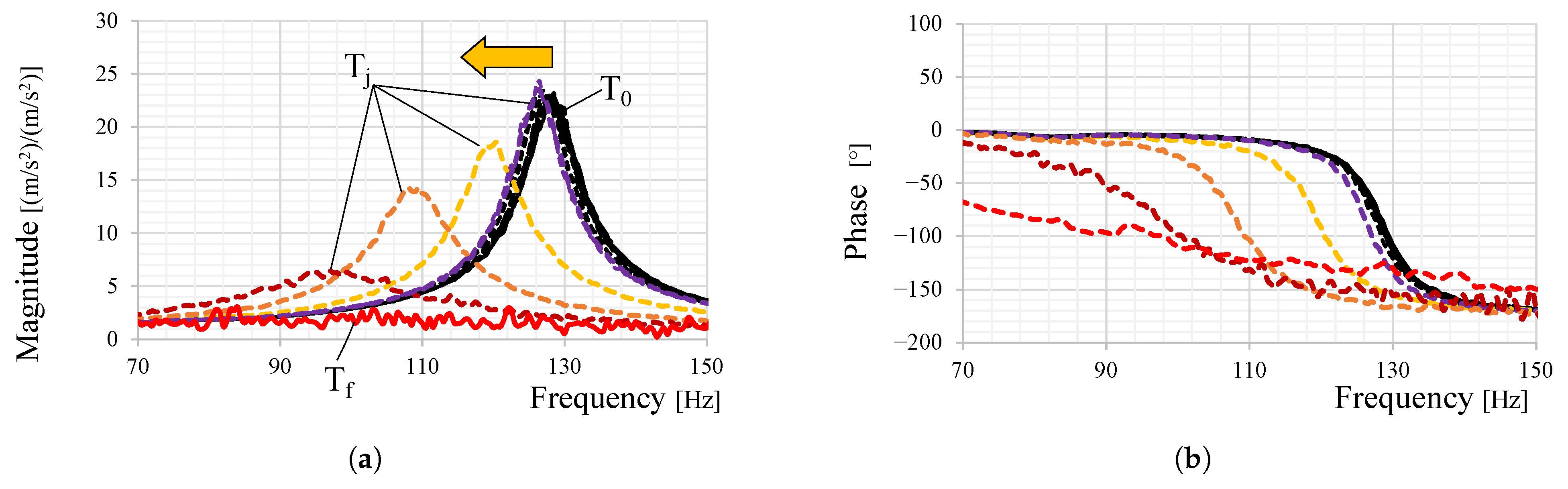
In the current study, the shift in both modal frequency and modal damping throughout the fatigue test is evaluated based on the recorded transmissibilities in order to detect the occurring fatigue-induced damage and establish a failure criterion for the TIM under study. Figure 8 illustrates the magnitude and phase of the recorded transmissibilities for a characteristic specimen (B02, beam No. 4, ASD = 4 (m//Hz). Clearly, the transmissibilities are continuously shifted to lower frequencies throughout the test. Two domains may be distinguished based on the recorded transmissibilities: one in which the frequency is constant to slowly decreasing with a slight increase in the amplitude and a second for which both frequency and amplitude are diminishing drastically.
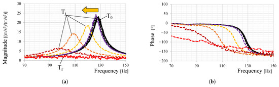
Figure 8.
Characteristic monitoring of the transmissibility’s magnitude (a) and phase (b) throughout the fatigue test for one specimen (B02, beam No. 4) at a chosen load level (ASD = 4 (m//Hz). denotes the reference transmissibility measured at the start of the fatigue test. is measured during the test, indicating the shift in the natural frequency to lower frequencies. is the transmissibility measured when the total delamination occurs.
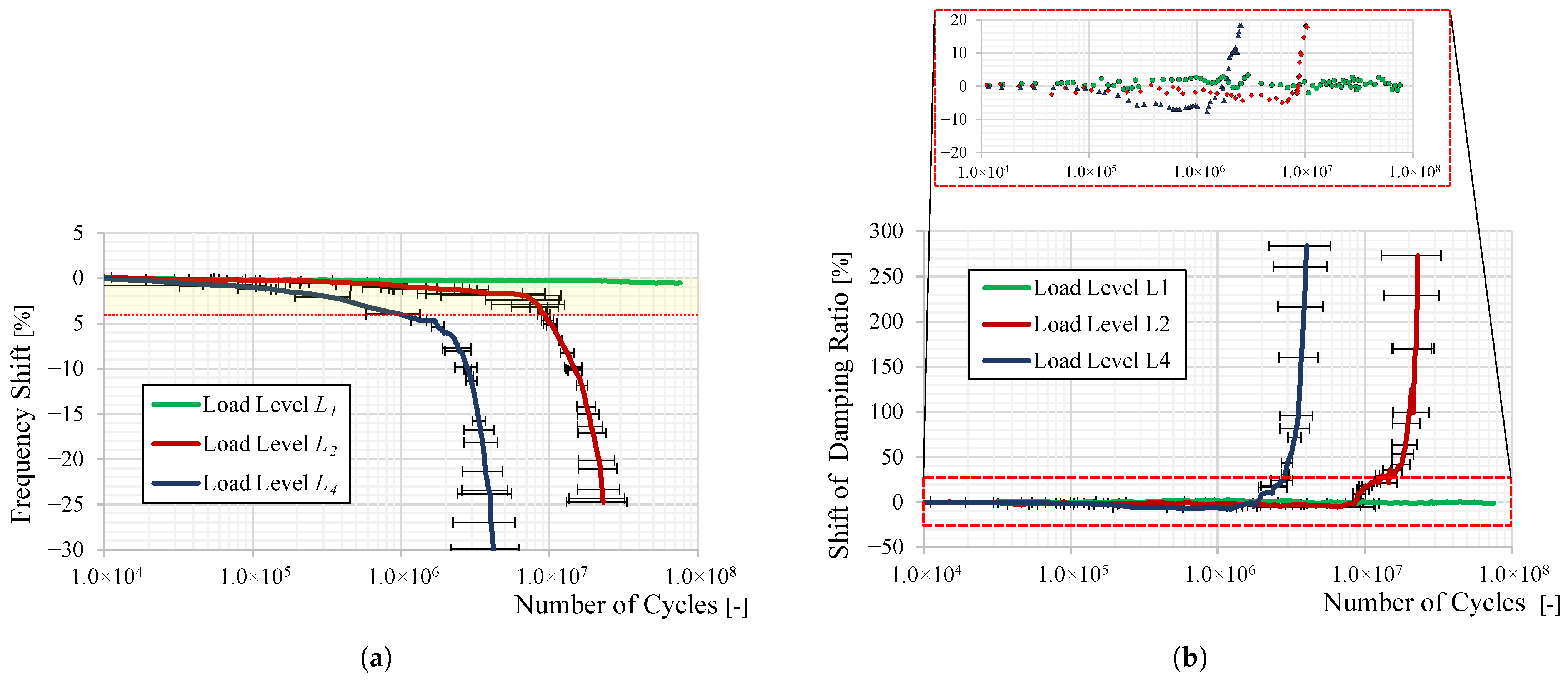
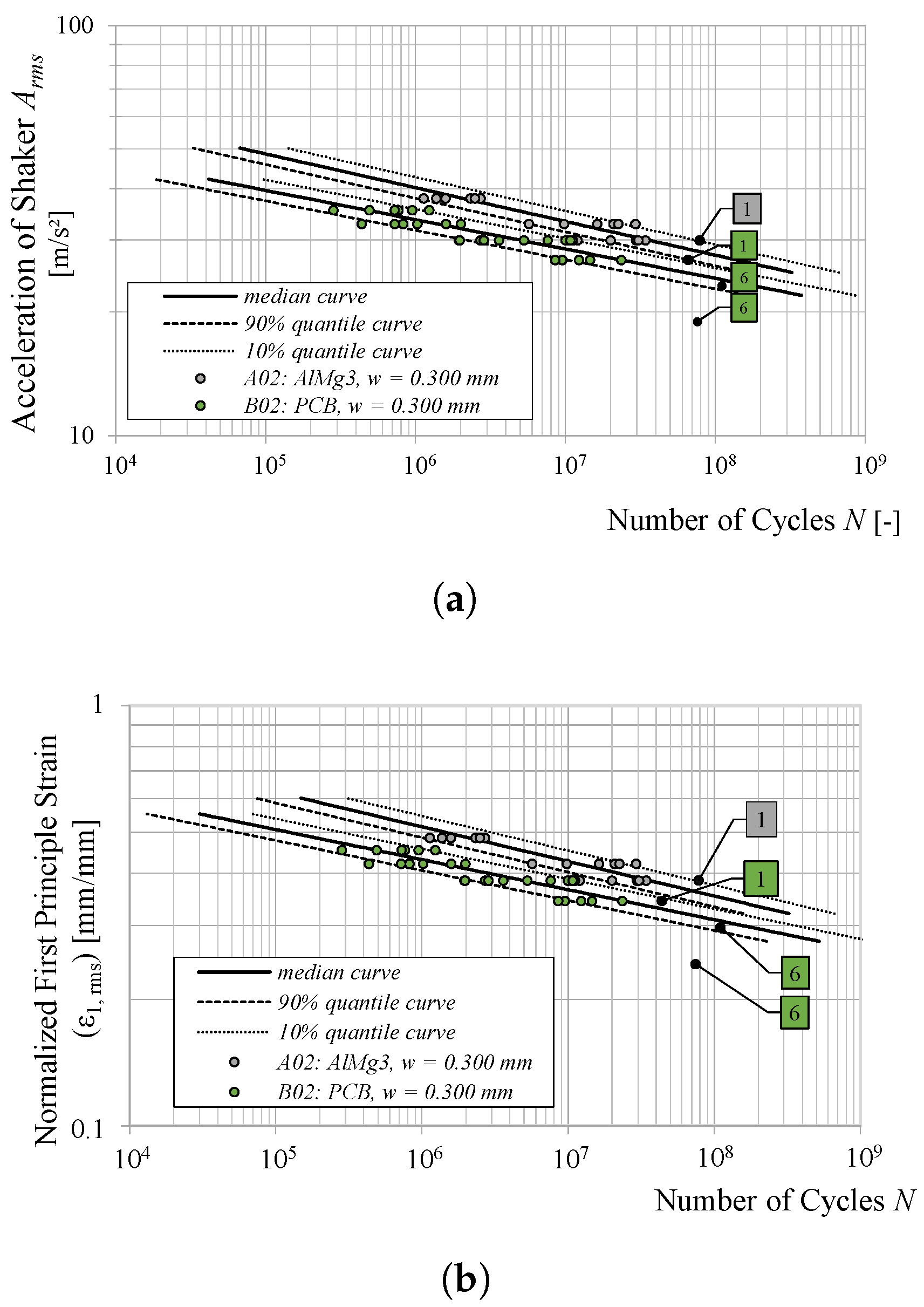
The progression of the monitored modal parameters (modal frequency and damping ratio) along the fatigue test is unveiled in Figure 9.

Figure 9.
Relative shift in the modal parameters: (a) resonant frequency and (b) damping ratio along the fatigue test for a characteristic beam from the B02 specimens at three load levels: , and , as defined in Table 6. Error bars are included representing variation among beams at the same load level.
The damping ratio is derived from the recorded transmissibilities according to the half-power bandwidth method as
where is the resonant frequency and are two particular frequencies from the left-hand and right-hand sides of , respectively, with a transmissibility amplitude of of the peak amplitude at [41]. The shift in the modal frequency and damping ratio is displayed as the percentage change relative to the initially measured values at ( and ). Additionally, the results are displayed for three different load levels and two beams each from the B02 specimens. Notably, a similar trend in frequency and damping shift is observed for other specimen types, including aluminum beams, as well as across different TIM thicknesses and temperature conditions.
Looking at the progression of the frequency shift in Figure 9a, one can distinguish two domains for the medium and high load levels ( and ): one with a slow change in the frequency followed by a second where the frequency shift is remarkably increasing. The lowest load level () has a rather flat behavior all along the fatigue test. The modal damping’s shift displayed in Figure 9b can similarly be divided into two domains: one with a flat curve progress and a second where the slope is almost vertical, indicating a drastic increase in the modal damping. An interesting finding from the modal damping curve progress is the existence of a transitional phase between the first and the second domain where the modal damping is actually decreasing, reaching a minimum and then starting to increase. Our interpretation of the above-identified domains in the curve progress is summarized in the following passage:
- (i)
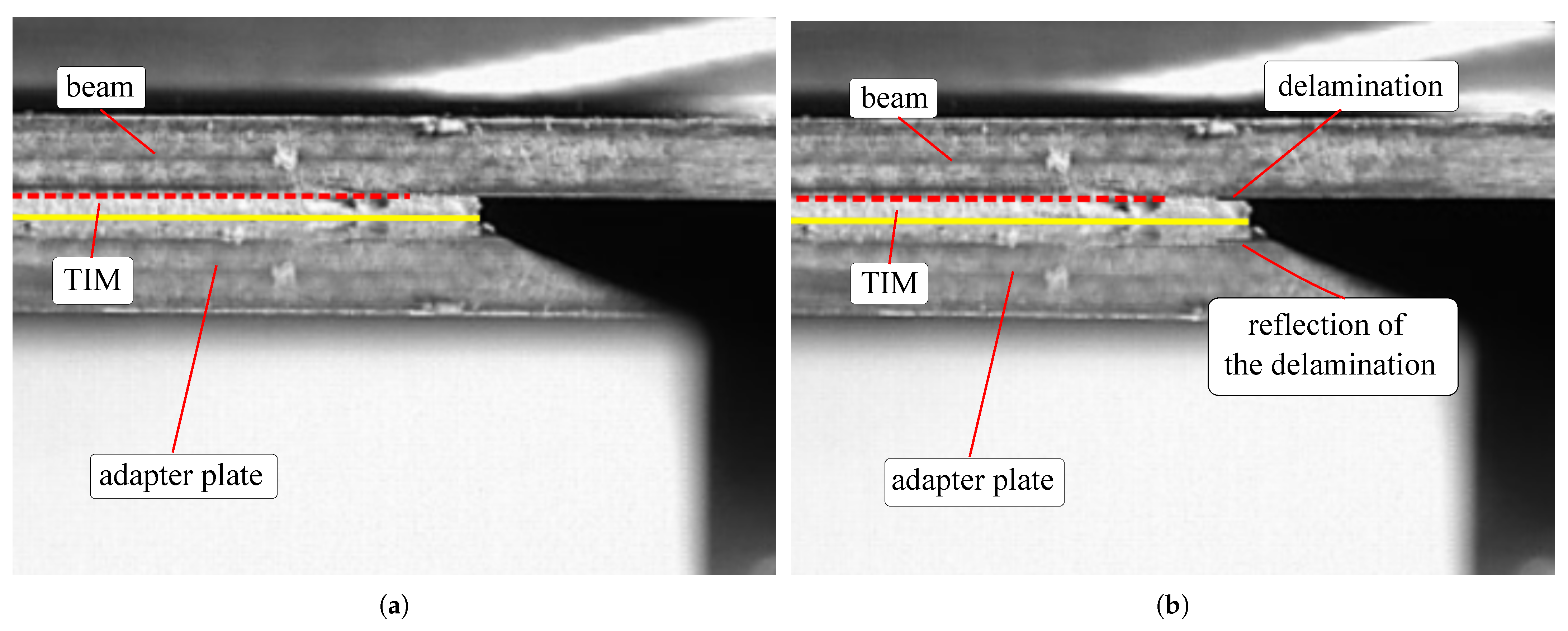
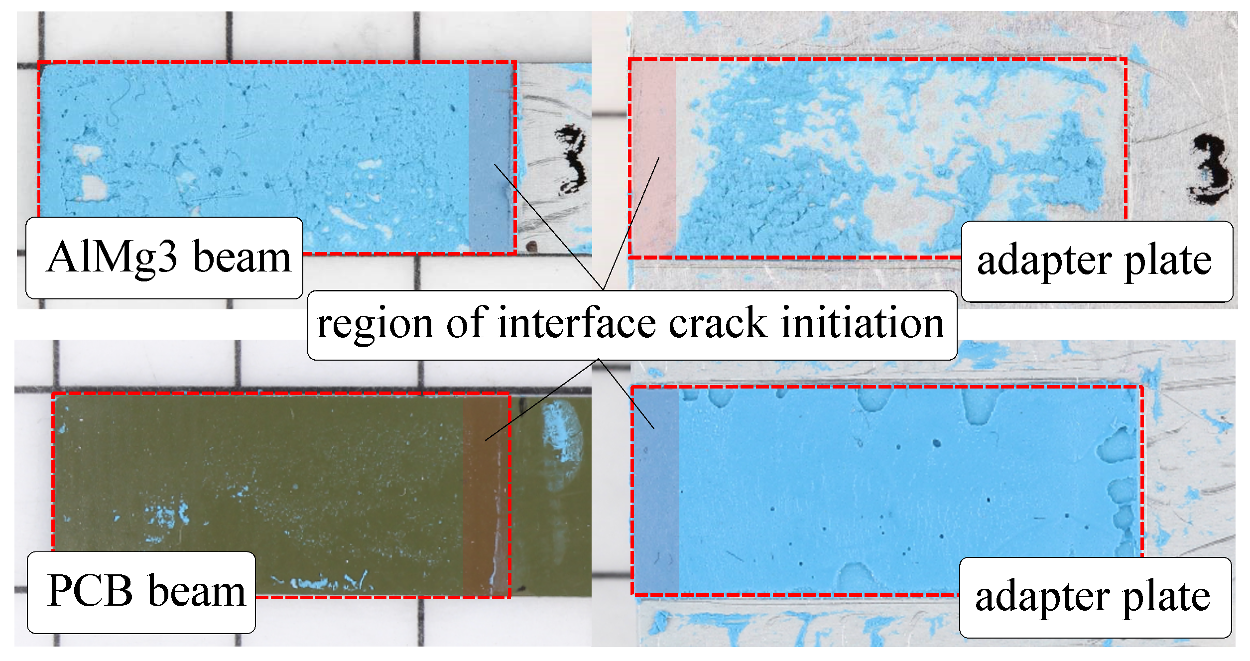
- Prior to evaluating the shift in the modal parameters and correlating it to possible damage in the tested adhesive assemblies, it is substantial to identify the failure pattern, i.e., mode. For this sake, two identification techniques were made use of, the first being the use of a high-speed camera (HSC) in situ to inspect the specimens for arising defects during the fatigue test. The second consists of visually analyzing the failure patterns of specimens tested until total failure. Figure 10 reveals the side view of the adhesive assembly beam—TIM plate at two different stages of the fatigue test for a B02 specimen tested at = 8 (m//Hz. Figure 10a is taken in the beginning of the test and Figure 10b after 3.5 h of the fatigue test, corresponding to around cycle counts and therefore located in the second domain of the modal parameters’ shift curves, corresponding to a rapid change in the frequency and damping. Surely, the HSC photographs confirm the presence of an interface crack, i.e., of an adhesive failure of the TIM, which seems to have been initiated at the TIM–beam interface. However, the use of HSC to detect the exact point of time and the location as well as to quantify the amount of damage is not best practice for very soft, elastomeric adhesive gap fillers such as the TIM under study. Therefore, we only relied on HSC to characterize the type and prove the presence of the damage during the fatigue test. The 100% delaminations, i.e., the total failure surfaces, are displayed in Figure 11 for both specimens with PCB as well as with aluminum beams. It may be noted that the PCB specimens exhibit some pores around the perimeter of the bonded area. However, these pores do not affect the frontal contact area, where delamination occurs. The findings are as follows: (1) All of the specimens show an adhesive failure, which starts in the frontal contact area (highlighted in red in Figure 11) and propagates toward the beam end. (2) Both aluminum as well as PCB beam specimens show the same adhesive failure pattern in the interface crack initiation area. Differences were detected, however, in the crack propagation pattern, which shows either a 100% adhesive failure for most of the B0x specimen or a mixed failure pattern for A0x specimens. Yet, the focus of this study is restricted to the characterization of the failure initiation. Therefore, the same failure mode can be assumed for all of the tested specimens, i.e., an adhesive interface delamination. (3) The adhesion fails typically at the PCB–TIM interface. For aluminum specimens, adhesive failures are predominantly observed at the adapter plate side. The main reason behind this observation is that the aluminum beams are chemically etched while the adapter plates are only cleaned using acetone. As for the PCB beams, they were not treated prior to the test. These remarks confirm the generally acknowledged observation stating the important role surface plays in the quality of the interface between adhesive and substrate in adhesive joints [21].
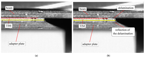 Figure 10. HSC photographs representing the side view of a representative beam from the specimens B02 during the fatigue test at = 8 (m//Hz in the beginning of the test (a) as well as after a couple of hours (b).
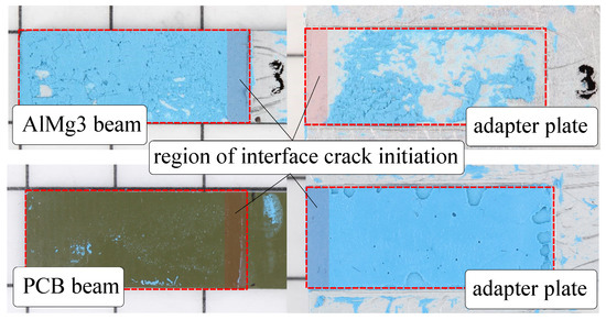 Figure 11. Failure patterns after 100% delamination was reached at the end of the fatigue test.
 - (ii)
- During the first domain of the curves in Figure 9 where the frequency is slowly diminishing and the damping is flat, no delamination has most likely occurred yet. The slight frequency shift corresponds to a stiffness loss, which may be linked to the softening of the TIM mainly due to internal changes in the micro-structure during the first cycles.
- (iii)
- The second domain where both modal parameters change in a rapid manner corresponds to a present macro-scale interface crack leading to a propagating adhesive failure, which decreases the overall stiffness and engenders friction-induced energy dissipation. This claim is confirmed by the HSC photographs in Figure 10.
- (iiii)
- The transitional area between the first and the second domain where both damping and frequency are slightly diminishing suggests the start of micro-scale defects which yet do not lead to increased damping because of the not yet prominent frictional effects. Although this claim cannot be proven using the HSC or by visually inspecting the failure pattern surfaces after test, this slight decrease in the modal damping during the fatigue process is observed in the literature such as in the works of [40,42].
To summarize, both tracking of the modal parameters as well as visual identification techniques were brought into play in the current study in order to detect, localize and characterize the occurring adhesive failure during the fatigue test. The results suggest that the interface crack initiation took place in the transitional domain between phase 1 and 2 of the modal parameters’ tracking curves in Figure 9. Yet, prior to deriving the fatigue life curves of the TIM, it is substantial to define a threshold of the frequency/damping shift, which can be applied as a failure criterion of the TIM. For this sake, an inverse correlation methodology of modal parameters’ shift to the interface crack length is introduced in the next section.
2.5. Correlation of the Shift in Modal Parameters to the Interface Crack Length
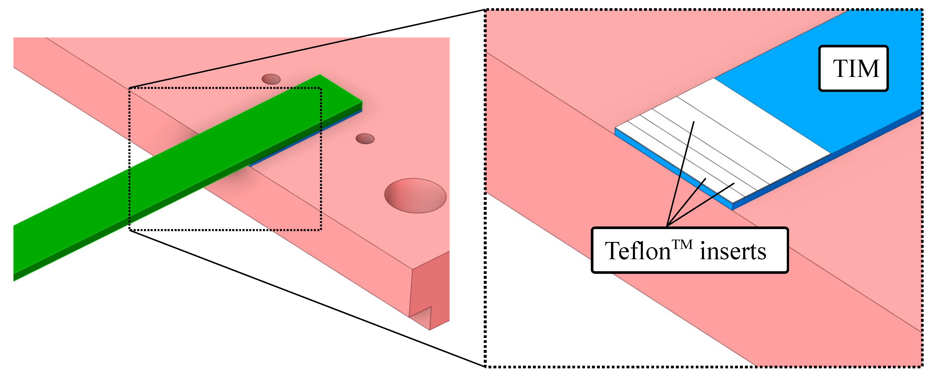
In order to correlate the observed shift in modal frequency and damping to the amount of fatigue-induced interface damage, the following inverse method is proposed: For B02 specimens, an artificial delamination, i.e., interface crack was generated using TeflonTM inserts placed in the frontal contact area to emulate the presence of a uniform macro-crack, as shown in Figure 12. Different lengths of the TeflonTM inserts were applied in order to identify a possible correlation of frequency and damping to the presence of an artificial crack. The emulated delamination lengths are 1, 2, 3, 5 and 8 mm. To account for the scattering effects, six beams are measured for each of the delamination lengths. In order to calculate the shift in the modal parameters, the measured average modal parameters of the artificially damaged specimens are compared to the average value of six “virgin” beams as well.
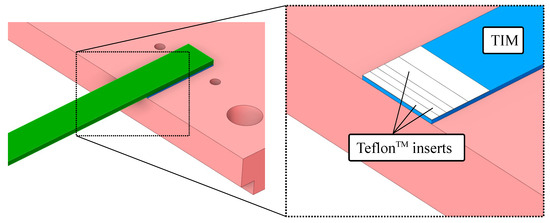
Figure 12.
Schematic view of the adopted specimens in the correlation study of shift in modal parameters to the amount of interface damage. TeflonTM inserts with different lengths are used to emulate the presence of an interface delamination.
The specimens are then mounted on an electrodynamic shaker using the same test setup as in the fatigue test illustrated in Figure 3, and the transmissibilities of each of the beam structures are measured at three different load levels: , and with AS = 0.1 (m//Hz, AS = 2 (m//Hz and AS = 4 (m//Hz. The frequency range of the white noise ASD excitation is the same as in the fatigue test. This investigation is performed under room temperature conditions RT = 23 °C.
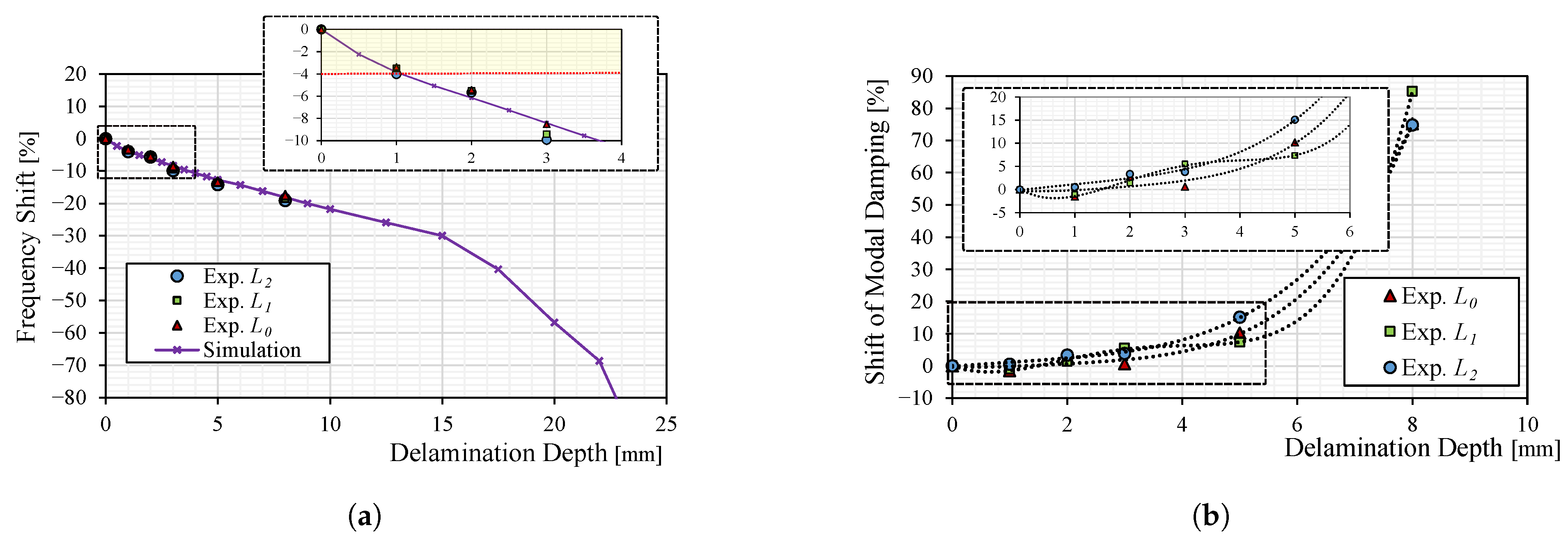
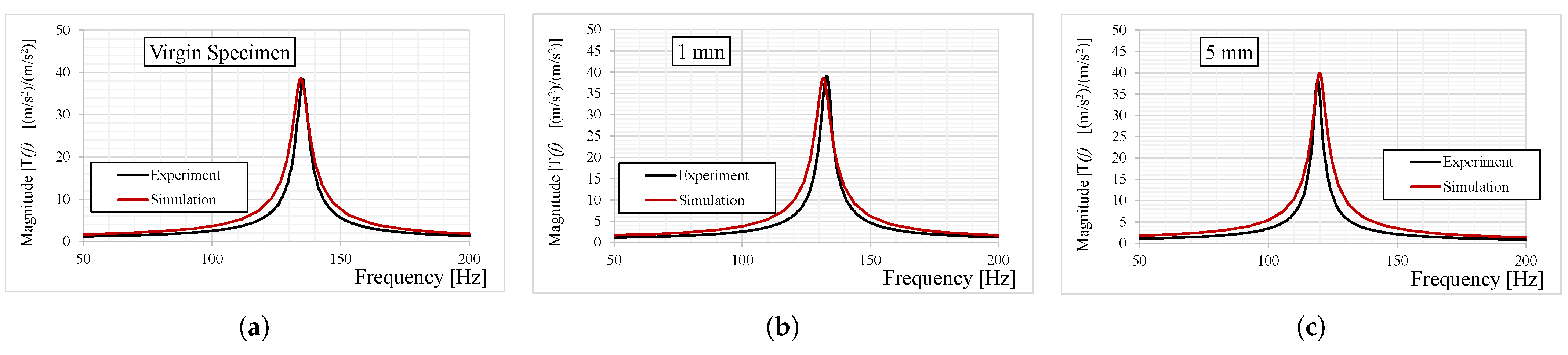
Figure 13 illustrates the plots of the shift in modal frequency and damping as a function of the artificial interface delamination length. A stiffness drop is visible in Figure 13a owing to the present artificial interface cracks and increasing with increased delamination length. A good agreement is observed for the results obtained from the resonance measurement to those from a finite-element analysis (FEA) where the delamination is modeled as no contact area and correlated to the drop in the modal frequency calculated from a modal analysis in the FE software (ANSYS 19.1, Ansys, Inc., Canonsburg, PA, USA) as illustrated in Figure 13a and Figure 14. This model can therefore predict the frequency drop if the delamination length is known a priori. However, its applicability is limited to the assumption of a uniform adhesive failure of the TIM, as observed in Figure 11 and modeled through the Teflon inserts. Additionally, the prediction is valid only for crack lengths up to 8 mm. Regarding the correlation between modal damping and delamination length, as shown in Figure 13b, a progressively rapid increase in modal damping is observed starting from a delamination length of approximately 2 to 3 mm. Although modal damping exhibits greater scatter compared to modal frequency, Figure 13b indicates that the damping measured at 1 mm for the load levels and is slightly lower than that of the virgin specimens before increasing progressively with further delamination growth.

Figure 13.
Output of the artificial delamination study: the shift in (a) modal frequency and (b) modal damping is correlated to the length/depth of the uniform interface delamination, and a failure criterion is established corresponding to a delamination length of 1 mm.
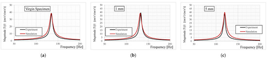
Figure 14.
Comparison of measured and computed transfer functions for (a) virgin specimens, (b) specimens with 1 mm delamination and (c) specimens with 5 mm delamination.
In reference to the presented results, a failure criterion of the tested specimens based on the frequency shift and guided by the behavior of the modal damping is opted for, namely a frequency shift of 4%, which corresponds to an occurring macro-scale interface crack. The corresponding delaminated surface amount matches that of a uniform artificial delamination of 1 mm.
2.6. Evaluation of the Local TIM Strains: Finite-Element (FE) Model Setup
Prior to establishing the fatigue curves based on the defined failure criterion, the local strains at the critical area of the TIM are evaluated through an FEA performed in ANSYS under the loading conditions of the fatigue test. Figure 15 illustrates the finite element model of the test structure. The beam and TIM are discretized using quadratic 3D 10-node tetrahedral structural solid elements (SOLID187) [43]. Given that the TIM is directly vulcanized onto both the beam and the plate, a multi-point constraint (MPC) is imposed at the beam–TIM and plate–TIM interfaces to ensure zero relative motion between the bonded elements. To replicate the shaker excitation, a random vibration base excitation is applied to the bottom surface of the base plate using the same ASD profiles listed in Table 6 while the material parameters of the TIM are taken from Table 3.
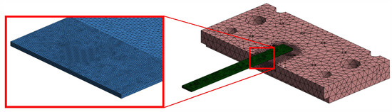
Figure 15.
Three-dimensional FE model of the test structure with detailed view of the meshing of the frontal area of the TIM where the highest strain levels are computed.
The effective strain parameter evaluated in this study is the first principal strain , which represents the maximum normal strain at a given point in the material. It occurs along the principal direction where the shear strain is zero and is computed as the largest eigenvalue of the strain tensor. The main mode shape of the jointed beam is transversal, inducing predominantly tensile stresses, making the first principal strain a suitable parameter for fatigue life prediction of the TIM under study.
It is well known that the computed strain values are highly sensitive to the mesh size. As the element size decreases, the calculated strain values tend to increase, primarily due to the stress/strain singularity at the interface of a bi-material system. To mitigate mesh dependence effects, a volume-weighted averaging method [44] is employed, allowing the calculation of an average effective strain across all elements in the critical area of the TIM. This approach ensures a more representative strain value and reduces numerical artifacts associated with mesh refinement. The volume-weighted average strain is expressed as
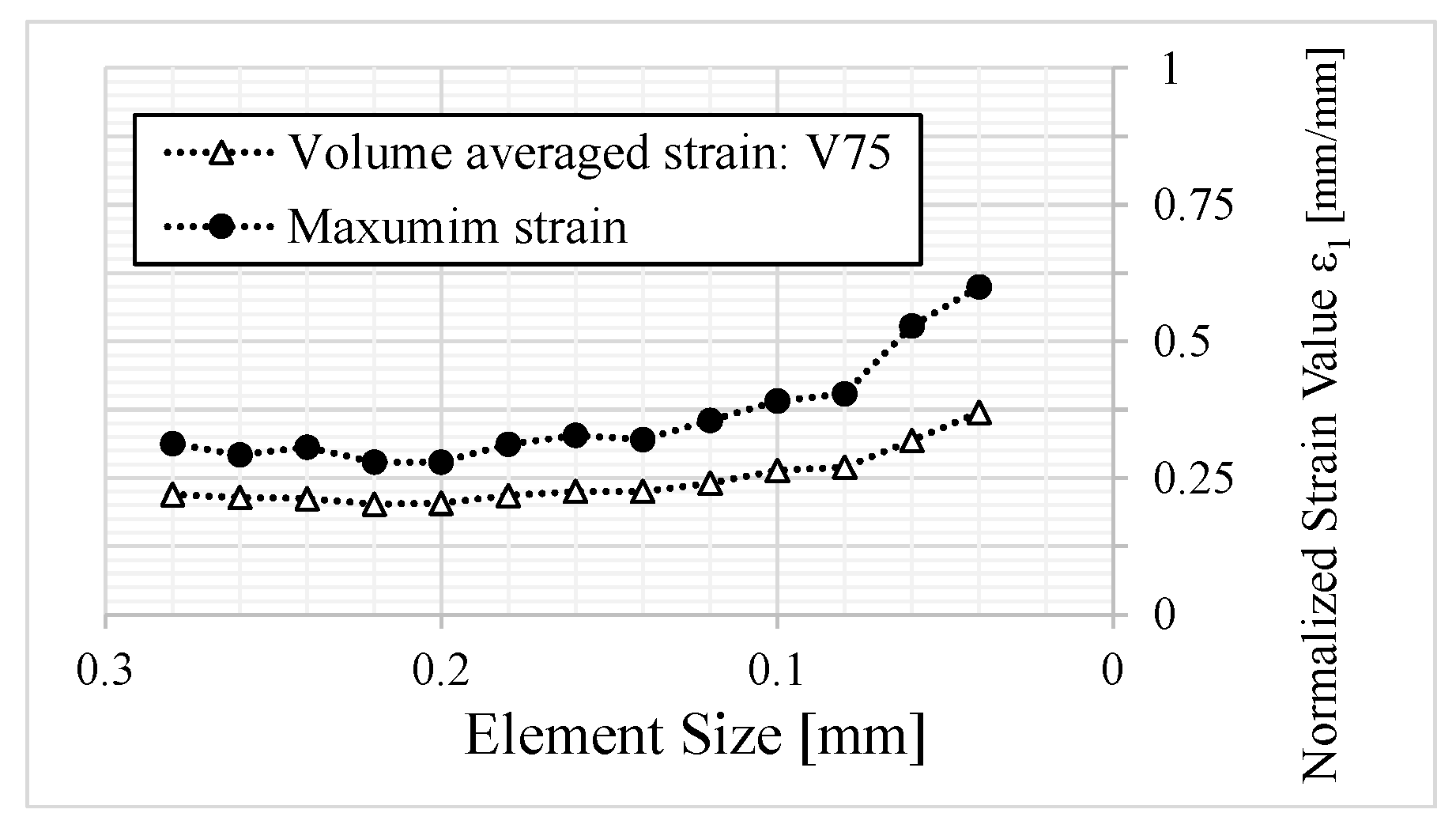
where is the volume-weighted average strain, is the strain in element i and is the volume of element i. The impact of the mesh size on the computed maximum and averaged strains computed for B02 specimens is illustrated in Figure 16. In Figure 17a, the distribution of in the frontal area of the TIM is illustrated. The location of the maximum strains correlates well with the observed location of the initiation of the delamination in Figure 10 and Figure 11. Figure 17b illustrates the so-called volume, which includes all elements with a strain value exceeding 75% of the maximum strain value in the evaluated TIM volume.

Figure 16.
Effect of mesh size on computed maximum and volume-weighted first principal strain in the TIM. The volume-averaged strain exhibits a flatter trend compared to the maximum strain. This suggests that the volume-averaging method attenuates singularity effects arising from geometric and material discontinuities.
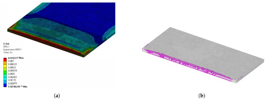
Figure 17.
Distribution of the first principle strain in the critical area of the TIM (a). The elements representing strain values beyond 75% of the maximum strain are highlighted in magenta (b).
Besides, the random vibration analysis of the fatigue test is based on the mode superposition (MSUP) method [45], a model order reduction technique that utilizes the natural frequencies and mode shapes obtained from a prior modal analysis to characterize the dynamic response of a structure in either the time or frequency domain. In this analysis, the strain power spectral density (PSD) is related to the shaker excitation ASD through the transfer function , which accounts for the frequency-dependent modal properties [45,46]:
The RMS value of the strain parameters is obtained by integrating the strain PSD over the frequency range of interest:
By applying Equation (6) to the computed during the random vibration analysis, the volume-averaged RMS values of the first principle strain are evaluated for all of the tested specimens at each of the load levels.
3. Results and Discussion: The Fatigue Life Curves, a Parametric Study
In this section, the main output of the current investigation, namely, the fatigue curves, is established and discussed, allowing a parameter study evaluating the effects of TIM thickness, surface quality and temperature on both the fatigue performance of the tested adhesive specimens and the HCF limit of the TIM.
3.1. Fatigue Curve Derivation
Both acceleration-based and strain-based fatigue curves are developed in the current work. The derived acceleration load capacities establish a relationship between the equivalent acceleration loads , measured by the control accelerometers on the adapter plate and the number of cycles to failure . Regarding the strain-based fatigue curves, they characterize the HCF limit of the TIM under study by correlating a local damage parameter—specifically, the first principal strain —to the number of cycles to failure . , and are referred to as such because they represent equivalent parameters derived under VA excitation, as depicted in Figure 7a.
The - relation can be expressed in terms of Basquin’s power law, of which the logarithmic representation yields [47]
where and are the characteristic Basquin’s parameters for the material under study, which are typically obtained from regression techniques taking into account the statistical uncertainties of both and at the different load levels of the fatigue test. The equivalent acceleration is typically taken as either the RMS acceleration or the peak acceleration . Both parameters can be estimated either from the time signal or from the ASD excitation spectrum measured by the control sensor (). Assuming to be stationary, zero mean and following a Gaussian distribution, these parameters are expressed as [47]
The factor hereby corresponds to the peak factor for a Gaussian process, which relates the expected peak amplitude to the RMS value. In this investigation, the - curves are plotted for the RMS acceleration . As for the number of cycles to failure, it is derived from the equivalent peak frequency of the beam’s first transversal mode, which is expressed as , where and are the second and fourth statistical moments of the beam’s acceleration response signal defined by the following equation:
Here, stands for the ASD spectrum measured by the response accelerometers placed toward the free end of the tested beams as in Figure 3. Due to the narrow bandwidth of , which is mainly dominated by the beam’s first transverse bending mode, the following relation can be assumed: , where is the resonant frequency of the beams for each of the tested specimens.
Based on Equation (9) and for , the - curves can furthermore be described through the following relation by conservatively assuming a single slope over the whole cycle range for the fatigue curve:
with and .
By substituting and by the computed volume-averaged RMS first principle strains , the Basquin power law of the - curves can be obtained as
with and .
Taking into account Equations (7) and (8), it can be shown that the RMS strain computed in an MSUP analysis is proportional to the RMS excitation acceleration of the shaker. These two parameters are related through the so-called acceleration-to-strain ratio. Consequently, a comparison of Equations (13) and (14) leads to the conclusion that
In other words, both the acceleration-based (-) and the strain-based fatigue curves (-) exhibit the same slope within the relevant HCF range.
The estimates of the fatigue life curve parameters are obtained using the maximum likelihood (ML) method, assuming a log-normal distribution for the number of cycles to failure at each tested load level. The regression is performed using the commercial software Minitab 22. Details regarding the derivation of fatigue life parameters considering statistical uncertainties with the ML method can be found in [20].
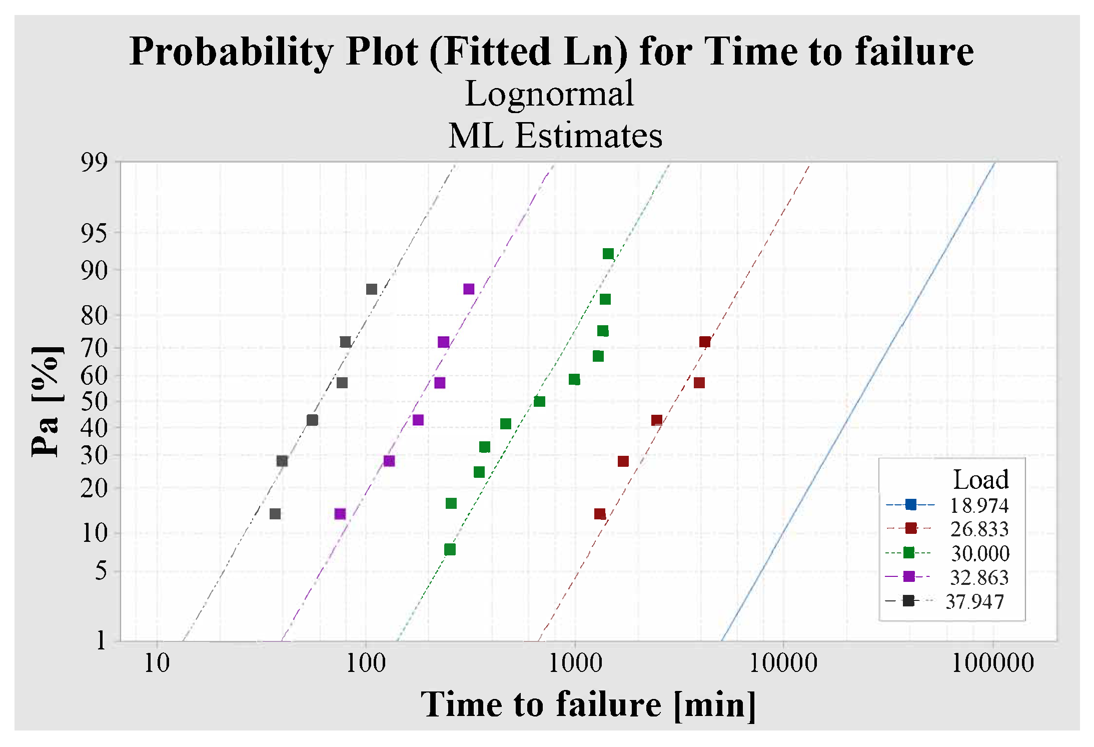
As illustrated in Figure 18, the time to failure, i.e., the number of cycles to failure from the fatigue test of B02 specimens, exhibits a strong correlation with the cumulative failure probability function () obtained under the assumption of a log-normal distribution.
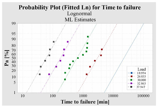
Figure 18.
Logarithmic-normal distribution of the time to failure from the fatigue test of a characteristic specimen (B02) for 5 different load levels ( in ) as defined in Table 6. Note that the lowest load level has only run-outs. Therefore, the distribution of the actual failures for the lowest load level does not match the estimated cumulative failure line.
The identified fatigue curve parameters for each of the tested specimen variants, i.e., the Basquin’s parameters ( and ) and the log-normal standard deviation s are summarized in Table 7. In the following, the fatigue life curves - and - are plotted, and the effect of the above-mentioned parameters is disclosed.
Table 7.
Basquin power law parameters and log-normal standard deviation of each the tested specimen’s variants obtained from ML estimation. The parameters and s are identical for both - and - curves.
3.2. Effect of the TIM Layer Thickness
The results presented in Figure 19a clearly indicate that an increase in bondline thickness leads to a longer fatigue life in the - curves. At a given shaker load level of m/, the predicted number of cycles to failure decreases by a factor of 0.2 when the thickness is reduced from 0.3 mm to 0.15 mm and increases by a factor of 4.5 when the thickness is increased from 0.3 mm to 0.5 mm. Notably, the slopes of the fatigue curves remain nearly identical across all tested thicknesses. This observation is consistent with previous findings reported in [26] for elastomeric adhesive joints, suggesting that the tested thicknesses in this study remain below the optimal adhesive thickness reported in the literature, beyond which fatigue performance deteriorates.
Figure 19.
- (a) and - (b) curves of the B0x specimens showing the effect of TIM layer thickness on the fatigue robustness of the tested adhesive assemblies.
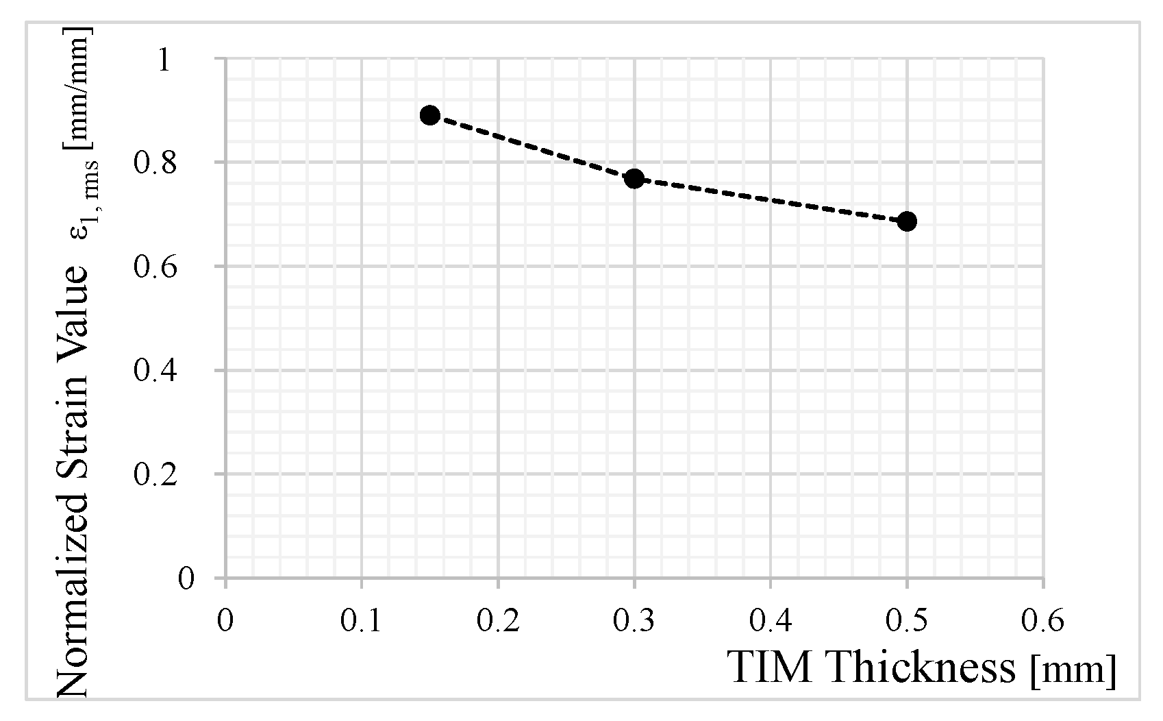
This trend can be attributed to the decrease in the volume-averaged first principal strain, , obtained from FEA as the thickness of the TIM increases. This relationship is illustrated in Figure 20 for an RMS shaker load of 30 m/, demonstrating that a thicker bondline results in lower strain magnitudes, thereby enhancing fatigue resistance.
Figure 20.
Effect of the thickness of the TIM layer on the volume-averaged strains from FEA under the same shaker acceleration load.
Taking this into account, the - curves of all the evaluated B0x specimens converge into a single - curve, as illustrated in Figure 19b. The Basquin’s parameters of this curve are = −13.12, = 12.99 and the log-normal standard deviation is s = 0.61. This confirms the robustness and suitability of as a local damage parameter for predicting the HCF performance of the TIM. Unlike acceleration-based fatigue analysis, which is highly influenced by geometric variations, the strain-based approach provides a more intrinsic measure of the TIM’s fatigue performance. This demonstrates that can effectively capture fatigue behavior regardless of changes in bondline thickness, provided that other influencing factors, such as temperature and surface quality, remain constant.
3.3. Effect of Adherend’s Surface Quality
Figure 21 illustrates the fatigue curves of specimens A02 and B02, both featuring a TIM thickness of m and tested under identical temperature conditions at room temperature (). The results indicate that the surface quality of the beams affects both the - and - curves of the tested adhesive assemblies.
Figure 21.
- (a) and - (b) curves plotted for the A02 and B02 specimens tested both under RT conditions to highlight the effect of the substrate surface on the HCF performance of the adhesive assemblies.
Specifically, the AlMg3 specimens, which were chemically etched before testing to enhance surface quality, exhibited superior fatigue performance compared to the PCB beams, which received no prior surface treatment in order to replicate real-world application conditions in engine ECUs. At a shaker load level of m/, the predicted number of cycles to failure, derived from both the - and - curves, increased by a factor of seven for the AlMg3 specimens compared to the untreated PCB beams.
Since the failure pattern of the tested specimens primarily corresponds to an adhesive failure in the frontal contact zone, as illustrated in Figure 11, the surface quality of the adherend plays a crucial role in determining the fatigue performance of the assemblies. This finding is further supported by the trend observed in the - curve plots in Figure 21b and aligns with previous research on the influence of surface treatments on adhesive joint durability, as reviewed in [21].
3.4. Effect of Ambient Temperature
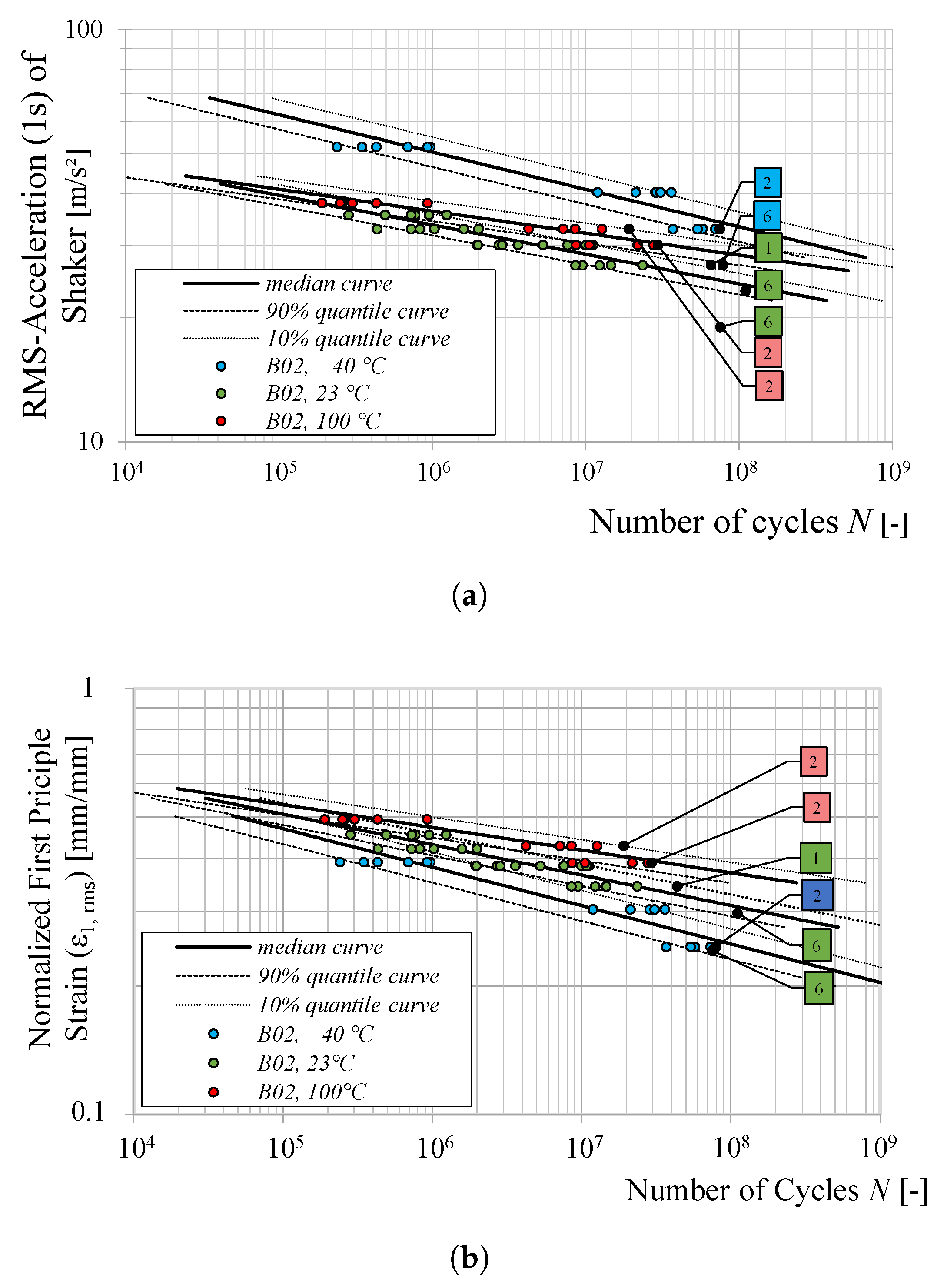
The acceleration fatigue curves (-) for B02 specimens tested at three different temperature conditions (23 °C, −40 °C and 100 °C) are shown in Figure 22a. The results indicate that specimens tested at −40 °C exhibit a significantly improved fatigue performance compared to those tested at 23 °C and 100 °C. However, the conventional trend of decreasing fatigue life with increasing temperature for structural epoxy adhesives is not strictly followed, as the fatigue performance at 100 °C does not degrade significantly compared to 23 °C. Additionally, the fatigue curve at 100 °C has a steeper slope, suggesting a more rapid transition between different fatigue regimes.
Figure 22.
- (a) and - (b) curves plotted for the B02 specimens tested under three different ambient temperature conditions: 23 °C, −40 °C and 100 °C.
This increased slope at 100 °C is likely influenced by measurement uncertainties, as the accelerometers used for transmissibility measurements deviate from their nominal response characteristics at elevated temperatures, particularly near 100 °C. As a result, some deviations in the fatigue life estimation at 100 °C must be interpreted with caution.
These inconsistencies indicate, furthermore, that the - curves may not be suitable for accurately assessing the influence of temperature on the fatigue strength of the studied adhesive assemblies, suggesting that the acceleration-based approach does not sufficiently capture the complex temperature-dependent failure mechanisms of the investigated TIM. Therefore, strain-based evaluation is necessary to provide a comprehensive understanding of the temperature effect.
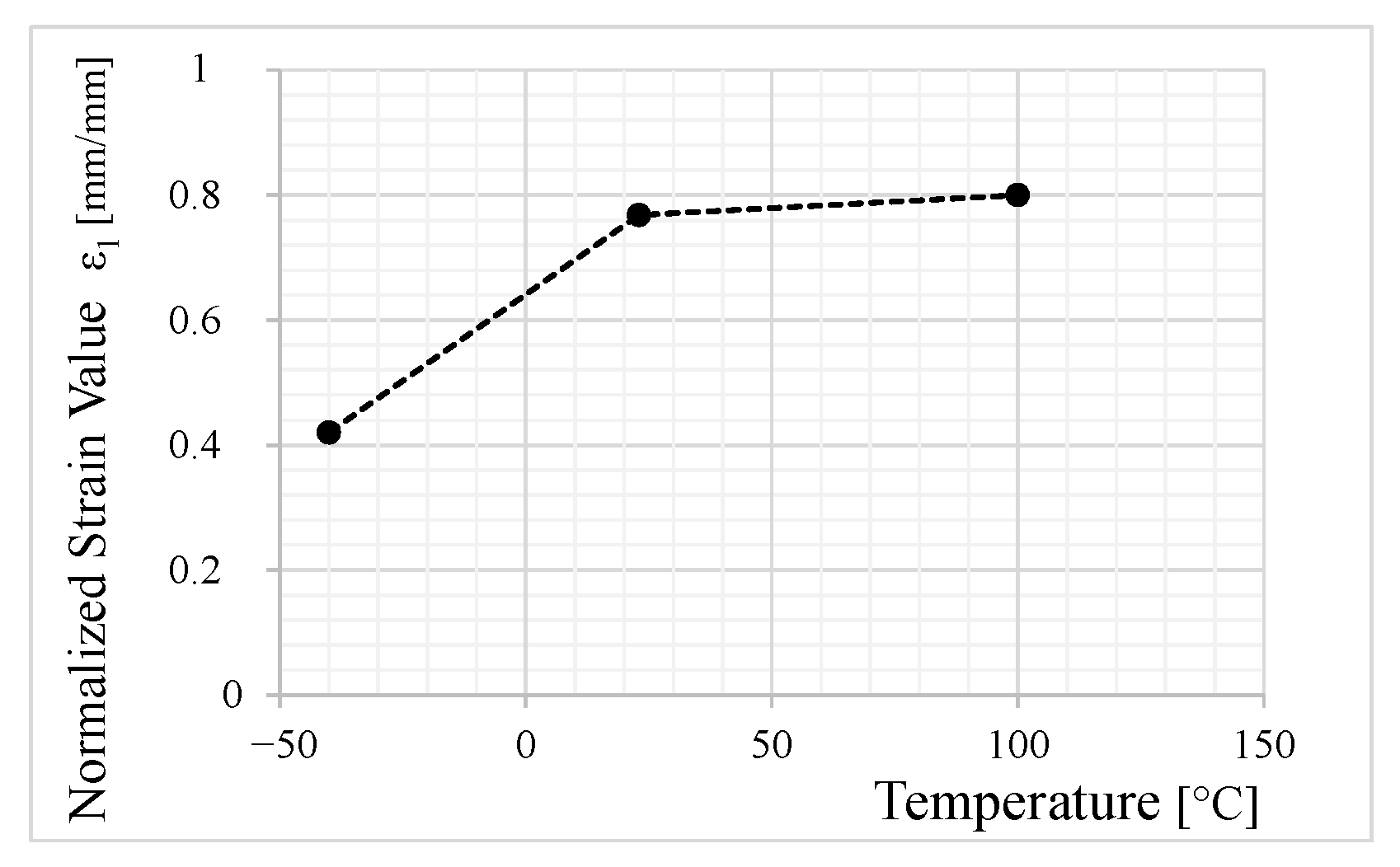
To further investigate the influence of temperature, the local volume-averaged first principal strain () is evaluated and presented in Figure 23. This is performed by considering the shift factors and material parameters listed in Table 2 and Table 3. Although specimens at −40 °C demonstrate superior fatigue performance, this behavior is primarily attributed to the increased stiffness of the TIM at lower temperatures, which in turn reduces local strain magnitudes and extends the number of cycles to failure.
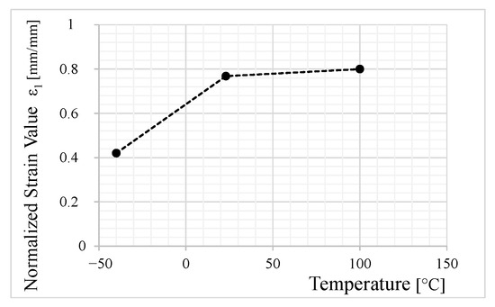
Figure 23.
Effect of ambient temperature on the volume-averaged strain from FEA under the same RMS shaker load of 30 m/.
Interestingly, the strain-based fatigue curves (-) plotted in Figure 22b reveal that at a fixed local strain amplitude ( mm/mm), the number of cycles to failure exhibits the following response to temperature changes:
- At −40 °C, the fatigue life decreases by a factor of 0.2 compared to 23 °C.
- At 100 °C, the fatigue life increases by a factor of eight relative to 23 °C.
This behavior suggests that conventional fatigue trends observed in structural epoxy adhesives may not be directly applicable to soft elastomeric silicones, such as the investigated TIM. The findings are consistent with previous research on elastomeric adhesives [26], specifically for one of the two tested adhesives in that study, further emphasizing the need for strain-based fatigue models when evaluating such materials. Nevertheless, while these results provide valuable insights, the influence of measurement uncertainties—particularly at elevated temperatures—must be considered when interpreting the findings.
4. Conclusions
This study presents a vibration-based testing approach for evaluating the HCF performance of TIMs used in automotive electronics. The methodology enables continuous excitation of the specimen’s first transversal mode using an electrodynamic shaker, allowing for efficient fatigue characterization under variable amplitude service conditions. The key findings of this study are summarized as follows:
- Failure criterion: a frequency shift of 4% is established as the failure criterion, corresponding to macro-delamination of the adhesive interface.
- Influence of thickness: the acceleration-based fatigue life decreases by a factor of 0.2 when reducing the TIM thickness from 0.3 mm to 0.15 mm and increases by a factor of 5.5 when increasing the thickness to 0.5 mm.
- Validation of as a local damage parameter: the first principal strain effectively describes the fatigue behavior across different TIM thicknesses while remaining independent of geometric variations, reinforcing its suitability for fatigue life prediction.
- Effect of surface quality: chemically etched AlMg3 specimens show an acceleration- and strain-based fatigue life increase by a factor of seven compared to untreated PCB specimens, highlighting the role of surface preparation in adhesion strength.
- Temperature influence: Strain-based fatigue life decreases by a factor of 0.2 at °C and increases by a factor of 8 at °C compared to the reference value at 23 °C. This trend deviates from the conventional behavior observed in structural epoxy adhesives, indicating a more complex temperature dependence of the fatigue performance in soft elastomeric TIMs.
Future research should aim to expand the tested temperature range beyond °C while incorporating intermediate temperatures to improve the resolution of temperature-dependent fatigue behavior. Additionally, validating the strain-based damage parameter for more complex adhesive geometries in real-world automotive applications will further enhance the robustness and applicability of the proposed methodology.
Author Contributions
Conceptualization, A.F., A.S., W.M.-H. and A.Z.; methodology, A.F., A.S., W.M.-H. and A.Z.; software, A.F., A.S. and W.M.-H.; validation, A.F.; formal analysis, A.F., A.S. and A.Z.; investigation, A.F.; resources, A.F., A.S., W.M.-H. and A.Z.; data curation, A.F., A.S., W.M.-H. and A.Z.; writing—original draft preparation, A.F.; writing—review and editing, A.F., A.S. and A.Z.; visualization, A.F.; supervision, A.S., W.M.-H. and A.Z.; project administration, A.S. and W.M.-H. All authors have read and agreed to the published version of the manuscript.
Funding
This research received no external funding.
Institutional Review Board Statement
Not applicable.
Informed Consent Statement
Not applicable.
Data Availability Statement
The measurement data presented in this paper are available upon request from the corresponding author after prior approval by Robert Bosch GmbH due to data privacy.
Conflicts of Interest
Authors Alaa Fezai, Anuj Sharma and Wolfgang Müller-Hirsch were employed by the company Robert Bosch GmbH. The remaining authors declare that the research was conducted in the absence of any commercial or financial relationships that could be construed as a potential conflict of interest.
References
- Fezai, A.; Sharma, A.; Mueller-Hirsch, W.; Zimmermann, A. Identification of the viscoelastic material parameters of soft thermal interface layers through forward and inverse measurement techniques. IEEE Trans. Instrum. Meas. 2020, 69, 4908–4918. [Google Scholar]
- Poshtan, E.A.; Hegde, S.; Roessle, A. Mechanical behavior of thermal interface materials in electronic components under dynamic loading conditions. In Proceedings of the ASME 2017 International Technical Conference and Exhibition on Packaging and Integration of Electronic and Photonic Microsystems, San Francisco, CA, USA, 29 August–1 September 2017. [Google Scholar]
- Due, J.; Robinson, A.J. Reliability of thermal interface materials: A review. Appl. Therm. Eng. 2013, 50, 455–463. [Google Scholar]
- Skuriat, R.; Li, J.F.; Agyakwa, P.A.; Mattey, N.; Evans, P.; Johnson, C.M. Degradation of thermal interface materials for high-temperature power electronics applications. Microelectron. Reliab. 2013, 53, 1933–1942. [Google Scholar] [CrossRef]
- Carlton, H.; Pense, D.; Huitink, D. Thermomechanical degradation of thermal interface materials: Accelerated test development and reliability analysis. J. Electron. Packag. 2020, 142, 031112. [Google Scholar]
- Stanzl-Tschegg, S. Very high cycle fatigue measuring techniques. Int. J. Fatigue 2014, 60, 2–17. [Google Scholar]
- Zhong, X.; Li, Y.; Wang, J.; Chen, M.; Liu, Z. Study of fatigue damage behavior in off-axis CFRP composites using digital image correlation technology. Heliyon 2024, 10, e25577. [Google Scholar]
- Boutar, Y.; Naïmi, S.; Achour, T.; Khenfer, L.; Feaugas, X. Cyclic fatigue testing: Assessment of polyurethane adhesive joints’ durability for bus structures’ aluminium assembly. J. Adv. Join. Process. 2021, 3, 100053. [Google Scholar]
- Costa, P.; Nwawe, R.; Soares, H.; Reis, L.; Freitas, M.; Chen, Y.; Montalvão, D. Review of multiaxial testing for very high cycle fatigue: From ‘conventional’ to ultrasonic machines. Machines 2020, 8, 25. [Google Scholar] [CrossRef]
- Adam, T.J.; Horst, P. Experimental investigation of the very high cycle fatigue of GFRP [90/0]s cross-ply specimens subjected to high-frequency four-point bending. Compos. Sci. Technol. 2014, 101, 62–70. [Google Scholar] [CrossRef]
- George, T.J.; Seidt, J.; Shen, M.H.H.; Nicholas, T.; Cross, C.J. Development of a novel vibration-based fatigue testing methodology. Int. J. Fatigue 2004, 26, 477–486. [Google Scholar]
- George, T.J.; Shen, S.M.H.H.; Scott-Emuakpor, O.; Nicholas, T.; Cross, C.J.; Calcaterra, J. Goodman diagram via vibration-based fatigue testing. J. Eng. Mater. Technol. 2005, 127, 58–64. [Google Scholar] [CrossRef]
- Cesnik, M.; Slavic, J.; Boltežar, M. Uninterrupted and accelerated vibrational fatigue testing with simultaneous monitoring of the natural frequency and damping. J. Sound Vib. 2012, 331, 5370–5382. [Google Scholar] [CrossRef]
- Khalij, L.; Gautrelet, C.; Guillet, A. Fatigue curves of a low carbon steel obtained from vibration experiments with an electrodynamic shaker. Mater. Des. 2015, 86, 640–648. [Google Scholar]
- Himmelbauer, A.; Tillmanns, M.; Winter, G.; Gruen, F.; Kiesling, C. A novel high-frequency fatigue testing methodology for small thin-walled structures in the HCF/VHCF regime. Int. J. Fatigue 2021, 146, 106146. [Google Scholar] [CrossRef]
- Kubit, A.; Zielecki, W.; Kaščák, Ľ.; Szawara, P. Experimental study of the impact of chamfer and fillet in the frontal edge of adherends on the fatigue properties of adhesive joints subjected to peel. Technol. Autom. Montażu 2023, 1, 3. [Google Scholar] [CrossRef]
- Ben Fekih, L.; Verlinden, O.; De Fruytier, C.; Kouroussis, G. New high cycle fatigue test facility of adhesively bonded ceramic electronic components. In Proceedings of the 15th European Conference on Spacecraft Structures, Materials and Environmental Testing, Noordwijk, The Netherlands, 28 May–1 June 2018. [Google Scholar]
- Ben Fekih, L.; Verlinden, O.; Kouroussis, G. Derivation of a fatigue damage law for an adhesive from in-situ bending tests. Eng. Fract. Mech. 2021, 45, 107587. [Google Scholar] [CrossRef]
- Stanzl-Tschegg, S.E.; Mayer, H.; Stich, A. Variable amplitude loading in the very high-cycle fatigue regime. Int. J. Fatigue Fract. Eng. Mater. Struct. 2002, 25, 887–896. [Google Scholar] [CrossRef]
- Johannesson, P.; Svensson, T.; de Maré, J. Fatigue life prediction based on variable amplitude tests’ methodology. Int. J. Fatigue 2005, 27, 954–965. [Google Scholar] [CrossRef]
- Abdel Wahab, M.M. Fatigue in adhesively bonded joints: A review. ISRN Mater. Sci. 2012, 2012, 746308. [Google Scholar] [CrossRef]
- Malekinejad, H.; Carbas, R.J.C.; Akhavan-Safar, A.; Marques, E.A.S.; Castro Sousa, F.; da Silva, L.F.M. Enhancing fatigue life and strength of adhesively bonded composite joints: A comprehensive review. Materials 2023, 16, 6468. [Google Scholar] [CrossRef]
- Tang, J.H.; Sridhar, I.; Srikanth, N. Static and fatigue failure analysis of adhesively bonded thick composite single lap joints. Compos. Sci. Technol. 2013, 86, 18–25. [Google Scholar]
- Sahin, R.; Akpinar, S. The effects of adherend thickness on the fatigue strength of adhesively bonded single-lap joints. Int. J. Adhes. Adhes. 2021, 107, 102845. [Google Scholar]
- Zamani, P.; Jaamialahmadi, A.; da Silva, L.F.M. Fatigue life evaluation of Al-GFRP bonded lap joints under four-point bending using strain-life criteria. Int. J. Adhes. Adhes. 2023, 122, 103338. [Google Scholar] [CrossRef]
- Banea, M.D.; da Silva, L.F.M. Static and fatigue behaviour of room temperature vulcanising silicone adhesives for high-temperature aerospace applications. Mater. Werkst. 2010, 41, 325. [Google Scholar]
- Kang, S.G.; Kim, M.G.; Kim, C.G. Evaluation of cryogenic performance of adhesives using composite-aluminum double-lap joints. Compos. Res. 2007, 79, 301–309. [Google Scholar]
- Tan, W.; Na, J.; Wang, G.; Xu, Q.; Shen, H.; Mu, W. The effects of service temperature on the fatigue behavior of a polyurethane adhesive joint. Int. J. Adhes. Adhes. 2021, 107, 102819. [Google Scholar]
- Houjou, K.; Shimamoto, K.; Akiyama, H. Effect of test temperature on the shear and fatigue strengths of epoxy adhesive joints. J. Adhes. 2022, 98, 2599–2617. [Google Scholar]
- Pritz, T. Five-parameter fractional derivatice model for polymeric damping materials. J. Sound Vib. 2003, 265, 935–952. [Google Scholar]
- Carneiro, V.H.; Puga, H. Temperature variability of Poisson’s ratio and its influence on the complex modulus determined by dynamic mechanical analysis. Technologies 2018, 6, 81. [Google Scholar] [CrossRef]
- Bauchau, O.A.; Craig, J.I. Euler-Bernoulli Beam Theory. In Structural Analysis: Solid Mechanics and Its Applications; Springer: Dordrecht, The Netherlands, 2009; Volume 163, pp. 173–221. [Google Scholar]
- Ingole, S.B.; Chatterjee, A. Vibration analysis of single lap adhesive joint: Experimental and analytical investigation. J. Vib. Control 2010, 17, 1547–1556. [Google Scholar]
- Gaßner, E. Festigkeitsversuche mit wiederholter Beanspruchung im Flugzeugbau. Luftwissen 1939, 6, 61–64. [Google Scholar]
- Gaßner, E. Auswirkung betriebsähnlicher Belastungsfolgen auf die Festigkeit von Flugzeugbauteilen. Jahrb. Deutsch. Luftfahrtforsch. 1941, 1, 472–483. [Google Scholar]
- Gaßner, E. Betriebsfestigkeit, eine Bemessungsgrundlage für Konstruktionsteile mit statistisch wechselnden Betriebsbeanspruchungen. Konstruktion 1954, 6, 97–104. [Google Scholar]
- Amzallag, C.; Gerey, J.P.; Robert, J.L.; Bahuaud, J. Standardization of the rainflow counting method for fatigue analysis. Int. J. Fatigue 1994, 16, 287–293. [Google Scholar]
- Doebling, S.; Farrar, C.; Prime, M. A summary review of vibration-based damage identification methods. Shock Vib. Dig. 1998, 30, 91–105. [Google Scholar]
- Fan, W.; Qiao, P. Vibration-based damage identification methods: A review and comparative study. Struct. Health Monit. 2010, 10, 83–111. [Google Scholar]
- Cao, M.S.; Sha, G.G.; Gao, Y.F.; Ostachowicz, W. Structural damage identification using damping: A compendium of uses and features. Smart Mater. Struct. 2017, 26, 043001. [Google Scholar]
- Bert, C.W. Material damping: An introductory review of mathematic measures and experimental technique. J. Sound Vib. 1973, 29, 129–153. [Google Scholar]
- Khoshmanesh, S. The effect of the fatigue damage accumulation process on the damping and stiffness properties of adhesively bonded composite structures. Compos. Struct. 2022, 287, 115328. [Google Scholar]
- ANSYS Mechanical User’s Guide, Release 19.1; ANSYS, Inc.: Canonsburg, PA, USA, 2018.
- Wong, T.E.; Palmieri, F.W.; Reed, B.A.; Fenger, H.S.; Cohen, H.M.; Teshiba, K.T. Durability/Reliability of BGA Solder Joints under Vibration Environment. In Proceedings of the IEEE 2000 Electronic Components and Technology Conference, Las Vegas, NV, USA, 21–24 May 2000; pp. 1083–1088. [Google Scholar]
- Maia, N.M.M.; Silva, J.M.M. Theoretical and Experimental Modal Analysis; Research Studies Press: Baldock, UK, 1997. [Google Scholar]
- Maniar, Y.; Konstantin, G.; Sharma, A.; Binkele, P.; Schmauder, S. Solder joint lifetime modeling under random vibrational load collectives. JOM 2020, 72, 898–905. [Google Scholar]
- Haibach, E. Betriebsfestigkeit: Verfahren und Daten zur Bauteilberechnung, 3rd ed.; Springer: Berlin/Heidelberg, Germany, 2006. [Google Scholar]


Disclaimer/Publisher’s Note: The statements, opinions and data contained in all publications are solely those of the individual author(s) and contributor(s) and not of MDPI and/or the editor(s). MDPI and/or the editor(s) disclaim responsibility for any injury to people or property resulting from any ideas, methods, instructions or products referred to in the content. |
© 2025 by the authors. Licensee MDPI, Basel, Switzerland. This article is an open access article distributed under the terms and conditions of the Creative Commons Attribution (CC BY) license (https://creativecommons.org/licenses/by/4.0/).