Abstract
In recent years, driver assistance systems in cars, buses, and trucks have become more common and powerful. In particular, the introduction of AI methods to sensors, signal fusion, and traffic recognition allows us to step forward from actual level-2 assistance to level-3 Advanced Driver Assistance Systems (ADAS), where driving becomes autonomous and responsibility shifts from the driver to the automobile manufacturers. This, however, requires a high-precision risk assessment of failure, which can only be achieved by extensive data acquisition and statistical analysis of real traffic scenarios (which is impossible to perform by humans). Therefore, critical driving situations have to be identified and classified automatically. This paper develops and compares two different strategies—a traditional rule-based approach derived from deterministic causal considerations, and an AI-based approach trained with idealized cut-in, cut-out, and cut-through maneuvers. Application to a 10-h measurement sequence on a German highway demonstrates that the latter has the higher performance, whereas the former misses some of the safety-relevant events to be identified.
1. Introduction
About 95% of traffic accidents are due to erroneous decision-making of the drivers [1]. Driver assistance systems may cut down the number of accidents if their reliability is higher than that of human drivers. However, as such assistance systems become more powerful, they additionally have to compensate for the effect that a confident driver will become less watchful. Reliability becomes even more of a critical issue when gradually switching from level-2 to level-3, or higher assistance [2], where automobile OEMs (original equipment manufacturers) must assume full responsibility for any failures of their control systems. Mercedes-Benz was the first to release an officially certified level-3 assistant for autonomous driving on German highways, called Drive Pilot [3,4]. Other major players, such as BMW and Volvo, are poised to introduce similar products with enhanced performance to the market.
High reliability and low failure rates will be essential for the acceptance of self-driving vehicles by both consumers and politicians. This, however, somehow contradicts the software architecture behind such products, as the realization of self-driving functionalities is closely correlated with the development of AI methods. In particular, the appearance of deep learning was a major game changer, also enforcing a major paradigm change compared to traditional product development: models are extracted from data correlations instead of causal deduction starting from proven principles. The more powerful such models become, the higher the interpretability of predictions lost [5]. To counteract this property, car manufacturers have to work on two fronts: (i) making AI algorithms safe enough for autonomous driving, and (ii) carefully assessing the failure rate of such systems.
The safety challenge cannot be tackled with traditional field testing since the mileage required for assessing the desired low failure rate would be much too high [6]. Therefore, software-in-the-loop simulation (SiL) is utilized, embedding the real ADAS and sensor models in virtual vehicle models [7,8,9]. To save costs, only critical traffic scenarios are simulated. The simulation will then provide conditional probabilities of failure of the ADAS w.r.t. to various scenarios. For a final assessment of the overall failure probability, the rate of occurrence of these scenarios has to be known.
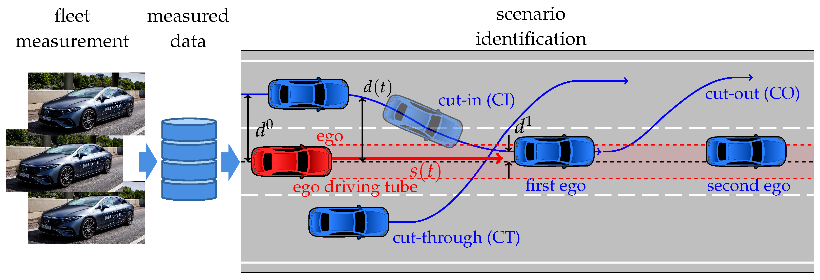
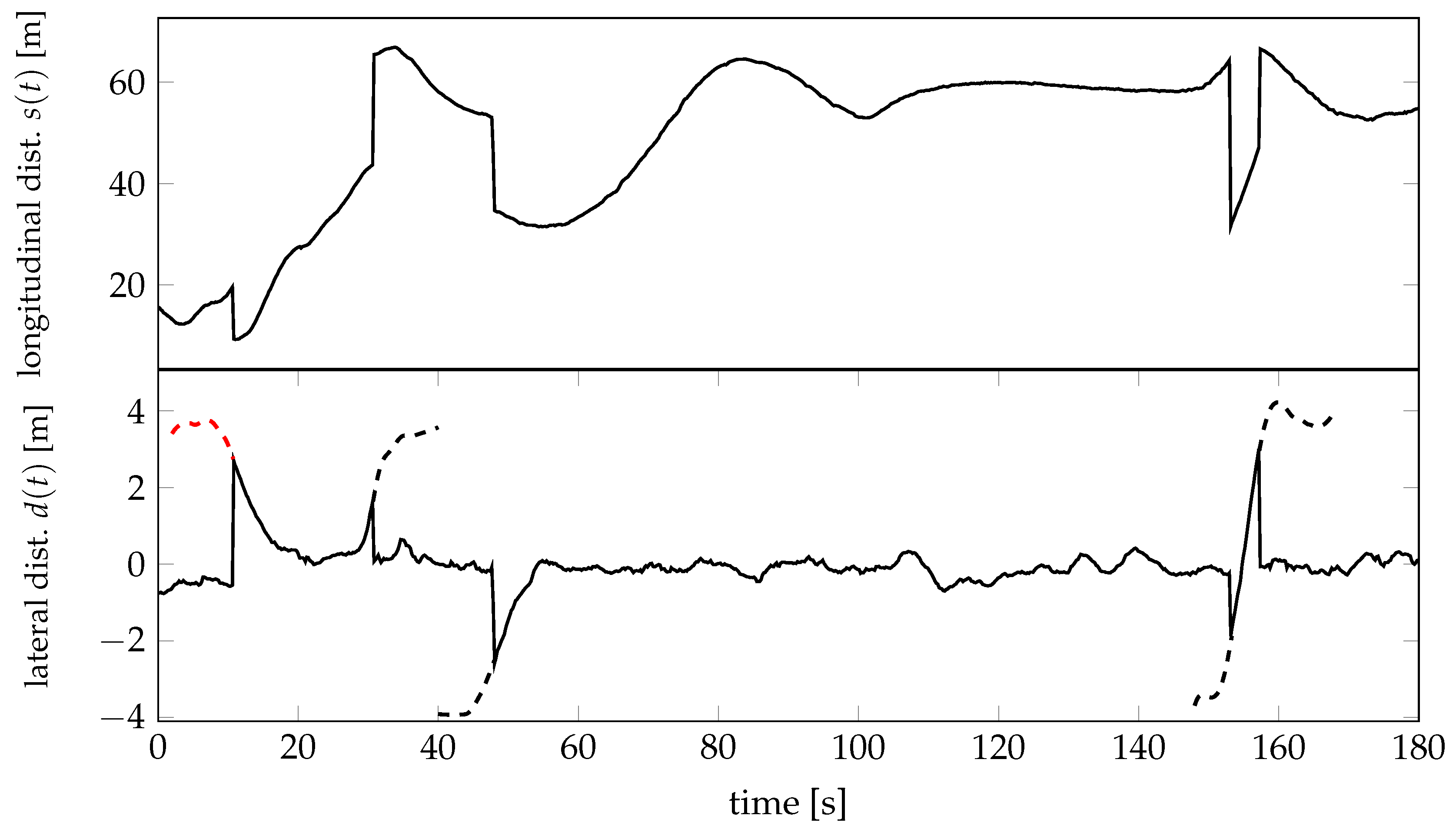
In close cooperation of automobile manufacturers with research institutions, the German research project PEGASUS [10] defined various logical scenarios with associated parameters. Here, the three scenarios—cut-in, cut-out, and cut-through—will be considered in more detail; see Figure 1. Mercedes-Benz AG has been collecting a rich dataset over the years via a large measurement fleet of vehicles, called ego, equipped with radar, lidar, and several cameras monitoring the traffic in the surrounding area. Only a minor subset of this data was analyzed by human engineers to extract characteristic time snippets and label them by the corresponding scenario class. To automatically find such events in a large dataset of measurements, an algorithmic search has to be performed. One possibility is to use pattern recognition of activities of the ego vehicle and the surrounding traffic [6,11,12,13,14]. The question, however, arises if the above-mentioned scenarios may simply be identified from measurements of the longitudinal distance between the ego and the first ego vehicle running ahead of the ego or from lateral distances of vehicles running on neighboring lanes; se Figure 2. The measurements are typically made with a measurement frequency of resulting in time steps of size . These raw signals are then preprocessed by filling up dropouts and smoothing signals by filtering. The lateral data are additionally corrected by eliminating road curvature effects [15].
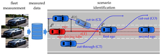
Figure 1.
Scenario identification from fleet measurements.
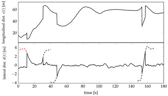
Figure 2.
Measured data for longitudinal distance and lateral distance .
Section 2 will use the measurement to detect cut-in, cut-out, and cut-through scenarios from sudden jumps when a car is entering or leaving the ego driving tube, see the upper plot in Figure 2. Rules will be derived from kinematic considerations and their impact on the longitudinal distance signal. Section 3 will build a detection and classification algorithm upon measurements of lateral distance and its characteristic time-behavior associated with the above maneuvers; see the lower plot in Figure 2. Preliminary studies [16] on several machine learning algorithms have shown that a strategy based on the Time Series Forest (TSF) approach [17] is suited best. As a machine learning approach, it requires training data, which is why Section 4 develops a simple procedure to generate idealized training maneuvers from pieces of time series. Both classification algorithms are tested and compared in Section 5 using the measurements of a 10-h ride on a German highway.
2. Rule-Based Classification Tree
The basis for deterministic scenario detection involves distance measurements in the longitudinal direction; see the upper plot in Figure 2. Whenever there is a sharp transition from high to low values, this indicates a cut-in (CI) maneuver. This occurs because the distance suddenly shifts from the first ego vehicle to a shorter distance to the vehicle that is cutting in. This vehicle enters the driving lane of the ego vehicle, becoming the new vehicle in front and reducing the gap; see Figure 1. In Figure 2, this occurs for . Subsequently, the ADAS reacts and enlarges the distance again to a proper, velocity-dependent distance. However, for , the distance value suddenly jumps from a low to a high value, indicating a cut-out (CO) maneuver, where the distance increases to the vehicle in front of the former first ego, called the second ego, after the latter has left the ego driving tube. Cut-through (CT) maneuvers combine both characteristics, the abrupt drop, and increase in within a short period of time, where the distance first reduces to the crossing vehicle and then back to the former first ego. This can be observed for 151–158 s.
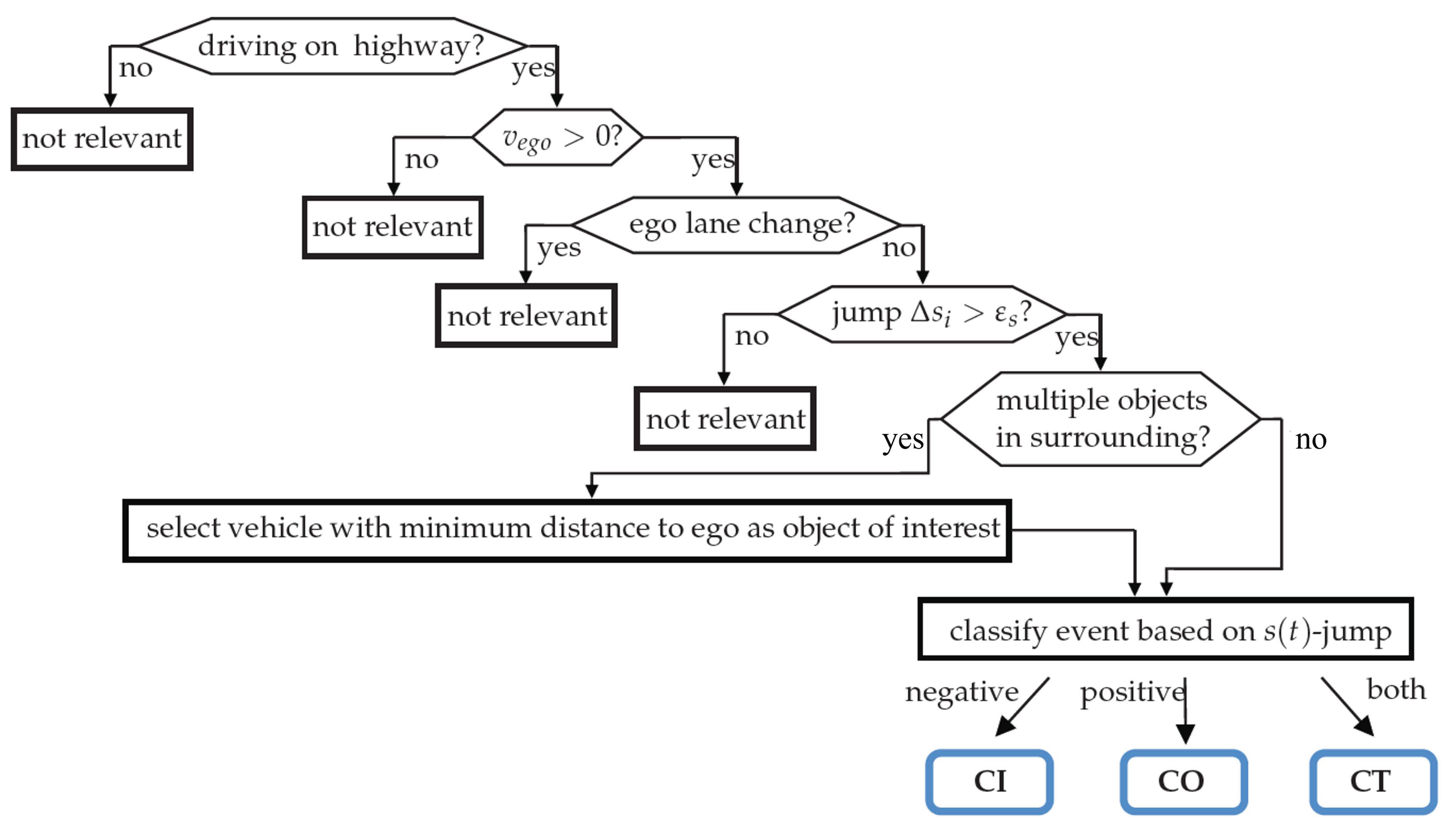
These relations may be embedded in a rule-based decision tree, as shown in Figure 3. The first three nodes exclude situations irrelevant to safety assessment. They check if the ego vehicle is driving on a highway with sufficient velocity since only then ADAS may take over control. Further ego lane changes are actually prohibited while driving in the level-3 mode. The more interesting fourth node detects jumps in the longitudinal distance to the vehicle driving ahead, where the difference of subsequent measurements has to exceed a user-defined threshold , i.e., . This could indicate one of the relevant scenarios (cut-in, cut-out, or cut-through), which may be directly classified depending on the sign of the jump if there exists only a single neighbor object in the subsequent measurement snippet. A cut-in maneuver suddenly shortens the distance yielding a negative jump; cut-out enlarges with a positive jump, and cut-through combines both jumps if they occur within a predefined time interval . In the following, and are chosen.

Figure 3.
Rule-based decision tree for scenario classification.
If multiple objects are located in the surrounding neighborhood of the ego vehicle and perform maneuvers, the distances between the ego and all objects of interest are measured at time points, , where a vehicle enters the ego-driving tube. The vehicle with the minimum distance is then the most critical and relevant one for scenario classification, whereas the other vehicles are ignored.
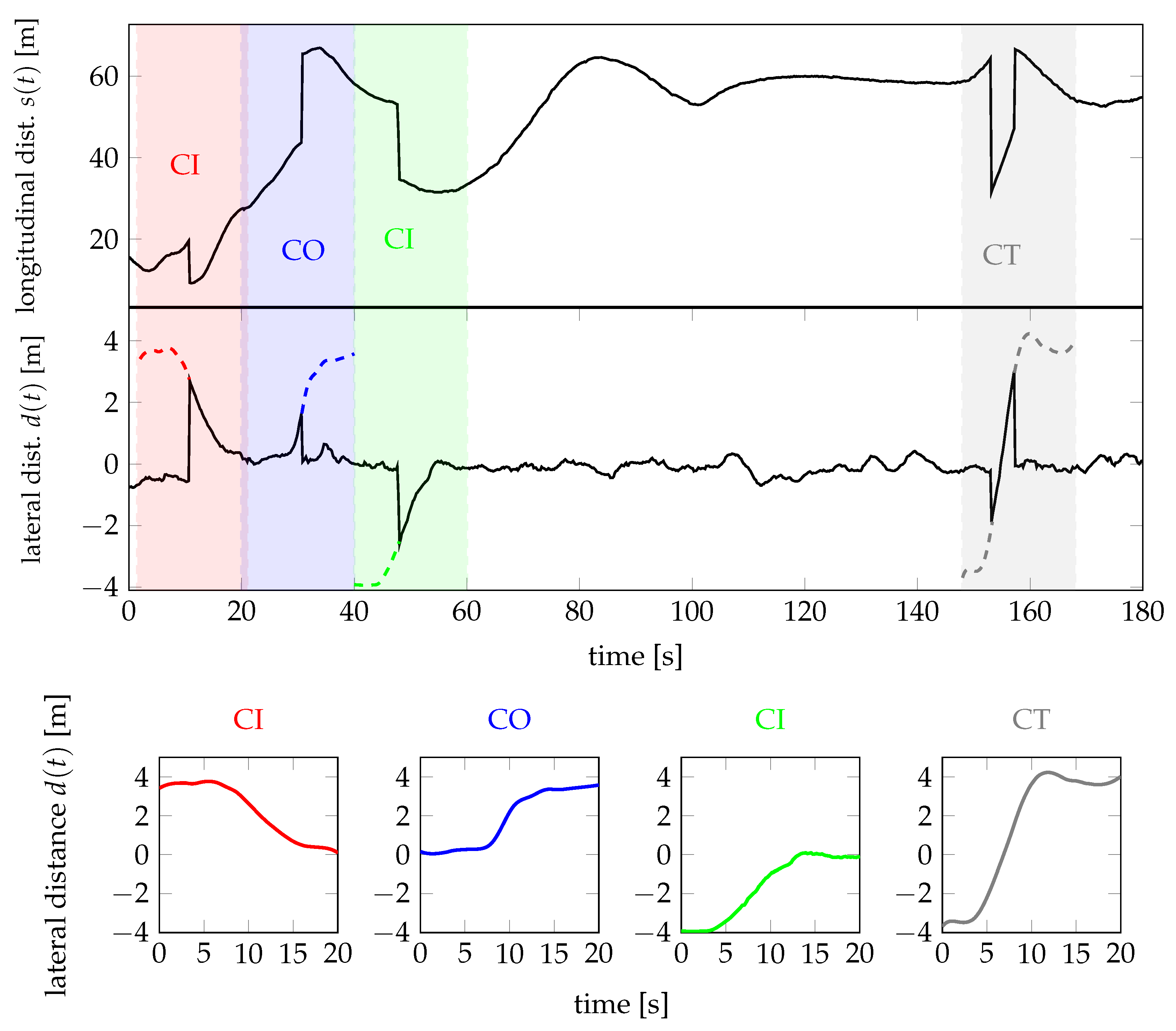
When applying the rule-based decision tree to the measurement section in Figure 2, it detects four relevant scenarios; see Figure 4. Additionally, it extracts corresponding snippets of the lateral distance around the respective time point when the -jump arises. They confirm the correct classification: in the first CI-event the cut-in vehicle enters from the left adjacent lane (distance about corresponding to the lane width), in the second CI-event from the right adjacent lane (distance about ). During cut-out, the vehicle leaves the ego lane to the left. Finally, the cut-through vehicle crosses from right to left.
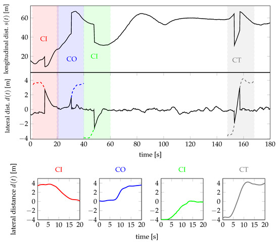
Figure 4.
Scenarios identified from distance measurement with corresponding snippets of lateral distance .
At first glance, what appears logical and has thus become state-of-the-art, has two drawbacks: First, noisy data, sensor dropouts, and ghost objects can disrupt the deterministic classification method described. Second, tolerances for jump-through () and cut-through durations () have to be chosen by experience, which may have a major impact on the robustness of classification. AI-based approaches, as discussed in the next section, are often more robust since they learn such parameters from training data.
3. AI-Based Classification Scheme
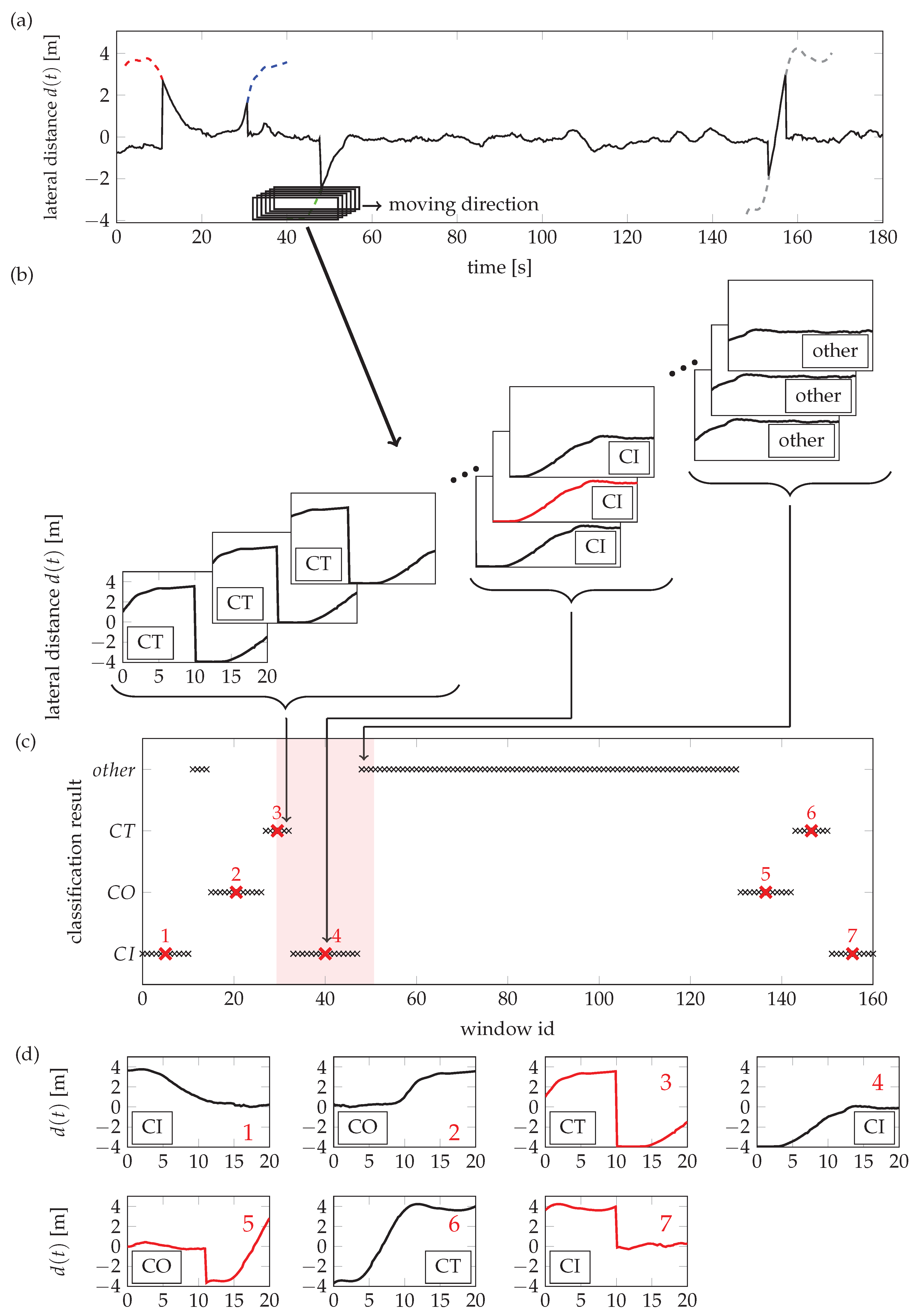
Analogous to the rule-based classification, the general conditions—such as the ego vehicle driving on a highway at sufficient velocity without performing a lane change—remain valid. But the main difference involves using the lateral distance behavior instead of for classification, to align more closely with real drivers, who primarily rely on lateral information to assess driving maneuvers [18]. To identify scenario classes from a long sequence of measured data , a moving window approach is applied; see Figure 5. The sliding window of length extracts pieces of the measurement to classify each window separately. Figure 5b shows some selected 20 s-sequences in the time range from to . From visual inspection, it can already be concluded that the trajectory pieces have different characteristics. The first three windows show a jump from almost 4 m to m in the lateral direction moving from right to left because the window moves in time from left to right. This may be considered a cut-through scenario. After some time, the jump diminishes, and the next three selected windows exhibit a gradual increase in already observed for a typical cut-in maneuver. Again, after a while, this increase shifts to the left, and the last three windows display an almost straight line, which does not fit any of the three defined scenarios and is, therefore, classified as “other”.
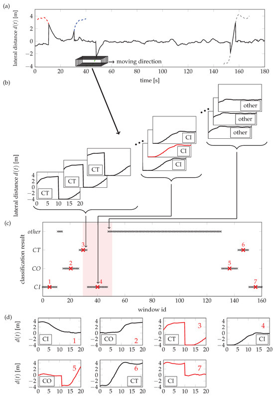
Figure 5.
Selected moving windows (b) extracted from a lateral distance measurement (a) and corresponding classification (c), which finally results in aggregated scenarios (d).
This procedure results in the classification sequence in Figure 5c, where the time-step of moving the window is , which is short enough to ensure that every driving maneuver is included in at least one of the analysis windows. Obviously, adjacent windows mostly yield the same classification results associated with the same event. Therefore, these sliding window classification results have to be aggregated in final scenario events. Here, we determine that a sequence of at least five identical classification results can be summarized as a single event, each with associated time frames centered around the time points marked by red crosses for the scenario classes CI, CO, and CT. In particular, the middle crosses are taken as references, respectively, where the final windows with the corresponding lateral trajectories of these events are illustrated in Figure 5d.
The kernel of the procedure is the assignment of a label to each window, W, referring to “cut-in”, “cut-out”, or “cut-through”, where classification is solely based on the measured lateral distances ; see Figure 6. If none of these scenarios apply to W, the label is assigned. Presuming a measurement frequency of , each window of length contains data points. Thus, the data basis of ssequences extracted from the measurement campaign of real driving tests is represented as a time series with an associated class c to be determined:
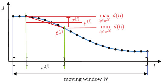
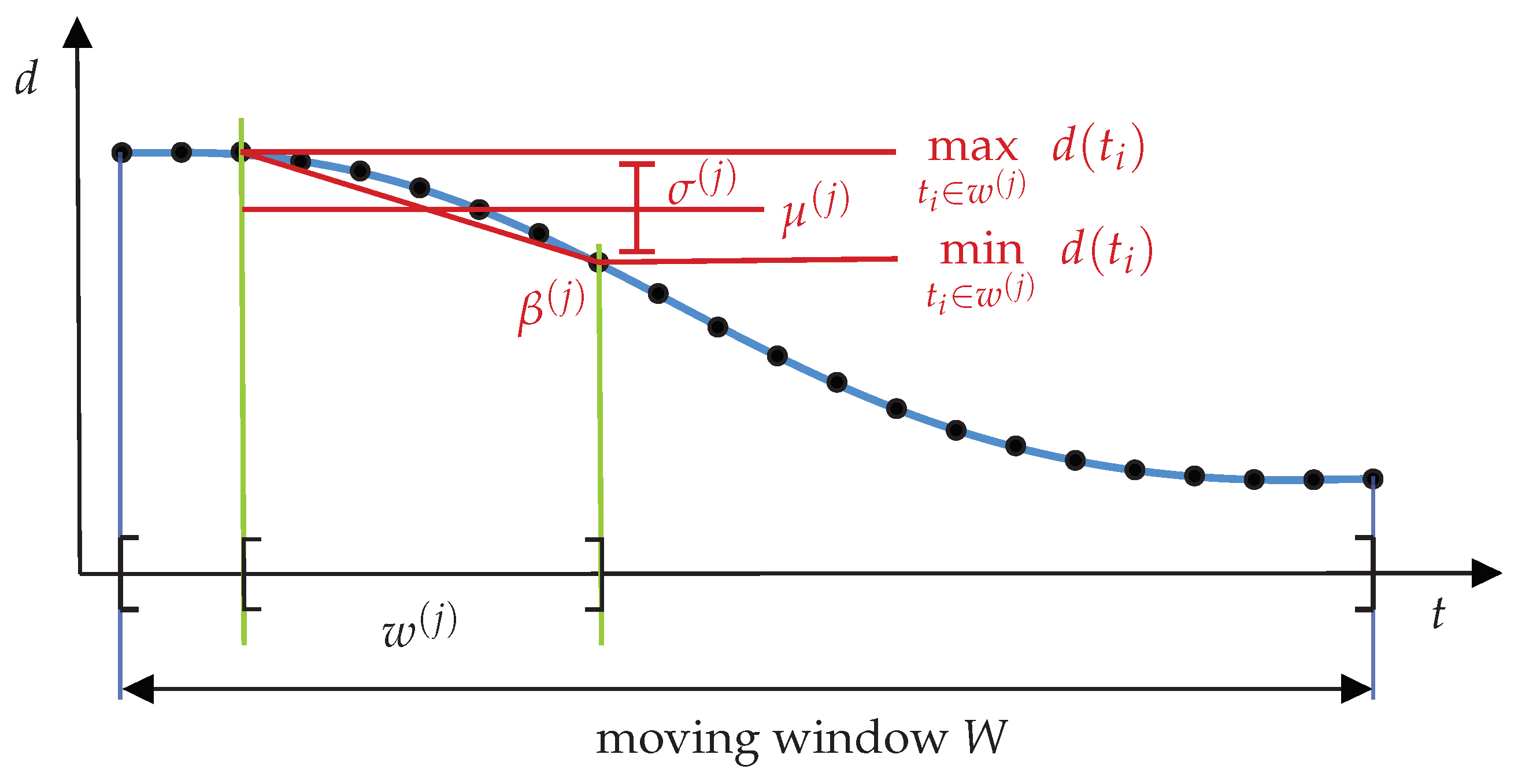
Figure 6.
Feature extraction from subinterval .
The applied classification method is based on the time series forest (TSF) approach [17] using a specific feature-engineering procedure. It splits the window, W, into randomly selected subintervals and assigns features like the mean, variance, and slope to each subinterval. In total, N subintervals are obtained by the so-called bagging, a randomized stripping of the whole window, W, into fixed, equal-width subintervals with replacement (here the bagging interval size is set to resulting in data points, c.f. Figure 6). In the following, interval features are considered and summarized in the feature vector, as follows:
The extracted features are the mean , standard deviation , and the slope of a regression line, Figure 6, as follows:
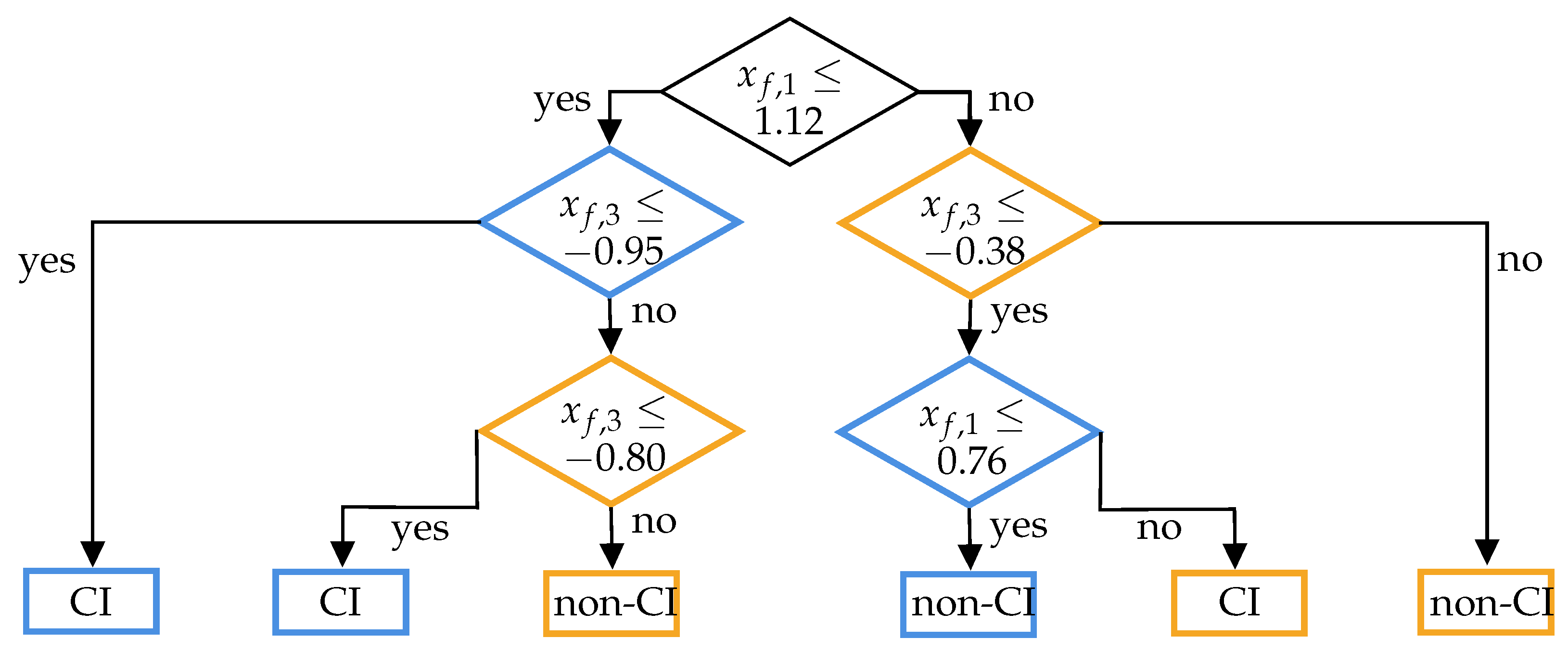
The calculations of the feature vectors are repeatedly applied to all randomly stripped subintervals, also known as sample generation. These samples are then used to build up a decision tree by learning splitting criteria as the base component of a classification tree (see, e.g., Figure 7), classifying CI or non-CI. When satisfying this decision rule, the respective instances of the sample are sent to the left child node (blue), otherwise, to the right child node (yellow). These subsets are then further split until either the subsets become too small or a user-defined maximum depth of the classification tree is reached (in the following, is limited to the maximum depth 8). In the example in Figure 7, is only three, and only binary classification is demonstrated for simplicity, although TSF is capable of dealing with multi-class problems, as in our application.
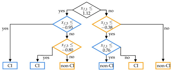
Figure 7.
Exemplary binary time series decision tree of depth , where non-CI represents CO, CT, or other.
Similar to the rule-based decision tree, time series trees also employ a top-down, recursive strategy. However, in this approach, each node independently learns the best-split feature, , and the best threshold for the split criterion from training, instead of pre-defining it. To achieve this, the best thresholds are found for all features , , individually by maximizing a combination of entropy gain and margin [17]. Let denote the maximum values of the split for each feature ; the one with the highest value is then selected for this specific node, as follows:
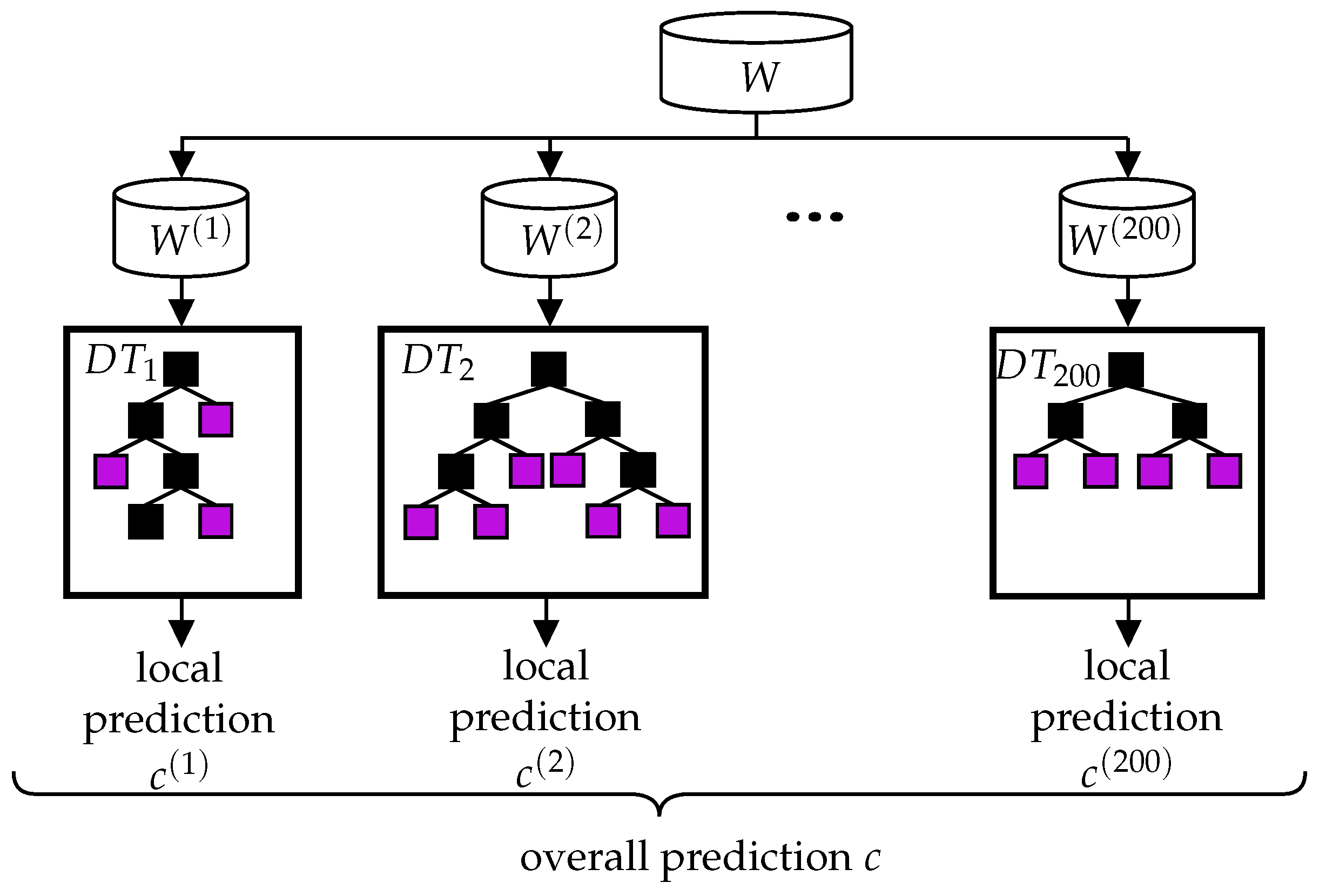
The resulting tree and, thus, its classification result, depends on the training set used. To make the classification procedure more robust, ensemble learning is applied: several different training subsets are generated by bagging, each resulting in its own decision tree . Applied to any test data, these multiple decision trees will predict different classification outcomes . To end up with a unique result, this tree ensemble is combined, such that the majority of classes define the final class c; see Figure 8. In this paper, the classification model consists of time series decision trees, each resulting from subintervals consisting of data points, respectively. In order to train the classification trees, a training set with hundreds of examples for each class is required. Since manual labeling of real measurement data is rather time-consuming, trajectories are generated as idealized driving maneuvers, as described in Section 4. The advantage is that the labels are known a priori.
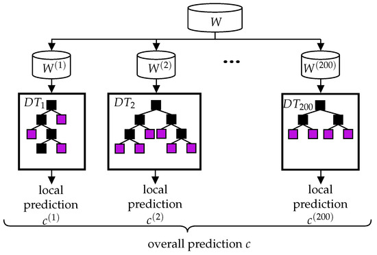
Figure 8.
Exemplary ensemble of time series decision trees with individual results combined to determine the final predicted class c.
The obtained time series-based machine learning classification model may then be applied to real-world data for automatic labeling of long-term measurements by performing classification of the moving windows. Figure 5 shows a short section of such a measurement with corresponding classification results. Similar to the rule-based approach in Figure 4, the AI approach finds the same four events labeled 1, 2, 4, and 6 in Figure 5c,d. In addition to the rule-based approach, the AI classification finds another three events, 3, 5, and 7, highlighted in red in Figure 5d. These, however, are misclassifications. The jump in event 3 from to was misinterpreted as a cut-through, although it actually resulted from switching the focus from the cut-in vehicle to another vehicle performing the next cut-in. Similarly, events 5 and 7 are misinterpretations of the different phases of a single cut-through maneuver 6. It should be noted that all these are speculations since the lack of causality in AI methods makes the interpretability of predictions difficult or even impossible. To be honest, the sequence in Figure 5 was selected to demonstrate the possibility of misclassification. Therefore, the above comparison should not be taken too seriously, but a rigorous assessment of the TSF performance must be made according to Section 5.
4. Generation of Idealized Maneuvers as Training Data
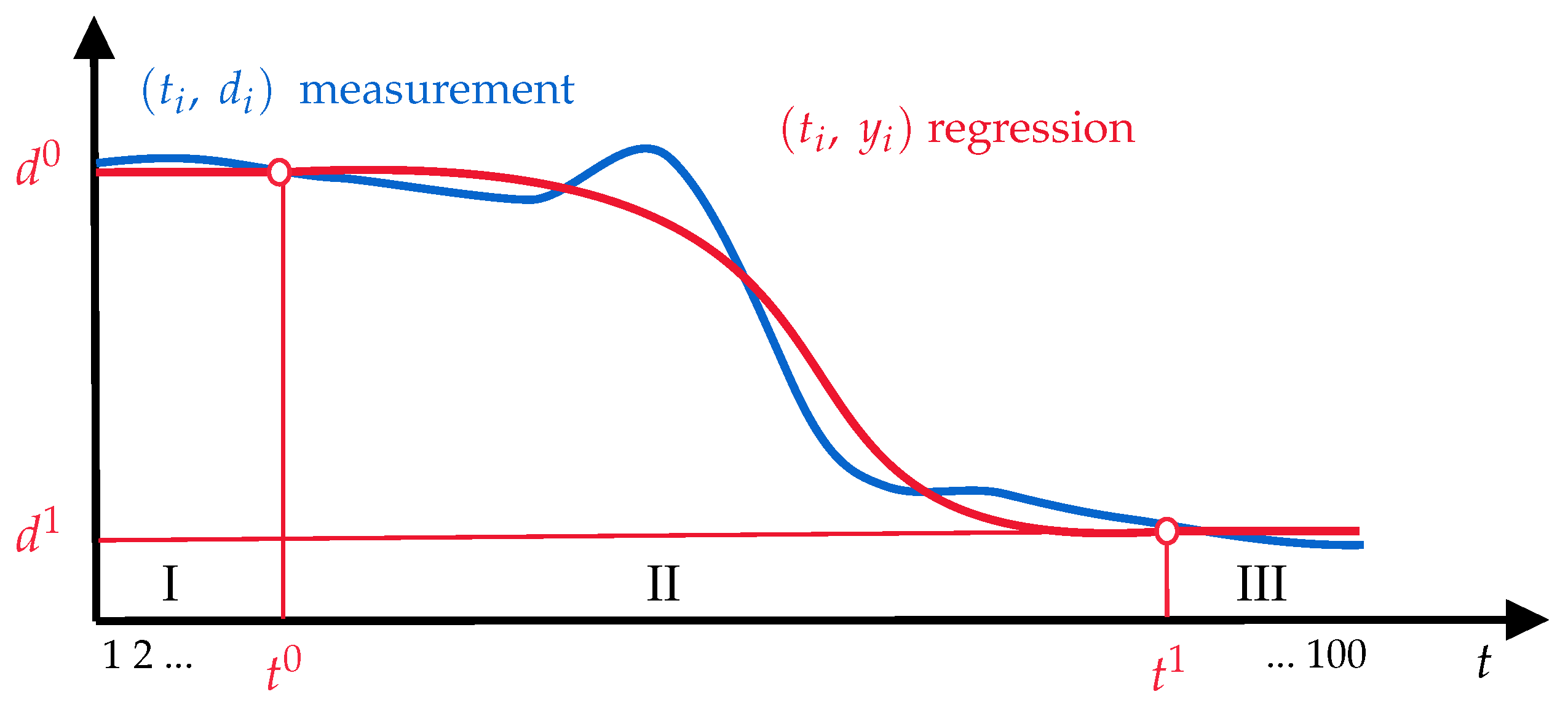
Apart from proper feature extraction and the model setup, the availability of enough training examples plays an important role in machine learning. In principle, labeled maneuvers obtained from measurements would be the best choice if available in a sufficient amount, otherwise, training data may be generated artificially [15,19]. To demonstrate the power of machine learning strategies, extremely idealized maneuvers will be used here, which are deduced from measurement data. According to Figure 1, ideal maneuvers have an initial phase with constant lateral distance , an S-shaped middle part describing the lane change, and a final phase that is also constant. Such an idealized cut-in maneuver is shown in Figure 9 as a red curve and can be described as a monotonic function by a cubic Hermite spline with three sections: (I) a constant initial phase with value for , (II) a 3rd-order polynomial, and (III) a constant end phase with value for . Realistic values of the parameters determining this curve may be obtained by regression of a measured lateral trajectory , ; see the blue curve in Figure 9. Thereby, we assume time snippets consisting of 100 points similar to the specifications above. For simplicity, the original real-time is substituted by its associated index, i, i.e.,
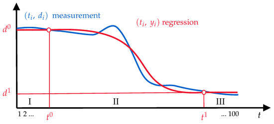
Figure 9.
Idealized parametric model (red) describing a real cut-in maneuver (blue) by the three-section Hermite-spline regression.
The goal of regression is to find the transition points as well as the initial and final position values in an optimal sense. This may be formulated as a two-stage minimization problem, as follows:
Generally, a cubic polynomial with boundaries and may be described as follows:
where
with
For zero derivatives , Equation (7) simplifies to the following:
Applied to the three sections, for the given and , we obtain the following regression conditions:
With submatrices , and , this may be summarized as an overestimated system of linear equations for , :
where , , . The values and then result from the least-squares solution and the final Hermite-spline is given as .
The outer minimization problem in Equation (6) may be solved by any nonlinear optimization algorithm. In order to avoid constraint (5) for and , we can re-parametrize the problem with normalized parameters :
A two-phase solution strategy is chosen, where global optimization by differential evolution [20] as the first phase is combined with local optimization by sequential quadratic programming (SQP), with the BFGS update [21] as the second phase to find global optimal parameters and, thus, , for the regression problem (6). Each evaluation of the cost function requires a least-square solution of Equation (12), which is pretty fast. Differential evolution explores the parameter space to find an initial guess for the global minimum, while the SQP algorithm refines this solution to find a more precise minimizer.
As a result, we find the idealized maneuvers in Figure 10. In the upper row, cut-in maneuvers start from lateral distances of about , which is the typical lane width of German highways, and ends at about . Cut-out maneuvers begin from the ego lane with and involve a lane change to the neighboring lane, ending with . Cut-through maneuvers typically start from the right neighboring lane with and proceed to . In the lower row, analogous training maneuvers from the other side are shown. Obviously, measurements reveal a wide variety of slow and fast lane changes, which have to be detected by the algorithms described in Section 2 and Section 3. It should be noted that the training samples in Figure 10 could also be generated artificially by randomly selecting the parameters , , , and within proper ranges and computing along Equation (11). Here, it should also be noted that the used classification model is trained with around 8000 generated trajectories from each scenario.
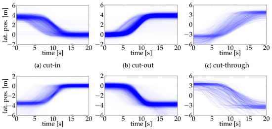
Figure 10.
Samples of idealized maneuvers: (a) cut-in from left and right, (b) cut-out to left and right, and (c) cut-through from right and left.
5. Comparison of Classification Strategies
In order to test the performances of the two classification approaches presented in Section 2 and Section 3 on real measurement data, 10 h of motorway driving are labeled, manually resulting in 77 cut-in (CI) maneuvers, 111 cut-out (CO) maneuvers, and 10 cut-through (CT) maneuvers. This is considered the ground truth. The classification quality of the rule-based (RB) decision tree and TSF-based model may then be assessed from the confusion matrices in Table 1.

Table 1.
Confusion matrix for the scenario classification.
The absolute frequencies or counts of predictions from the corresponding classification models, compared to the actual scenario events that occurred, are displayed. For example, Table 1a can be interpreted as follows: the rule-based decision tree correctly classifies 66 of the 77 CI events but misses 11 CI events and incorrectly classifies 8 other events as CI. Obviously, both approaches avoid misclassification with respect to the considered scenario types—CI, CO, or CT—but they do sometimes miss events or misclassify non-interesting measurement parts (= other) as one of the interesting scenarios. Therefore, cross-comparing the classification errors of the two classification models might be interesting. Table 2 highlights the falsely predicted events, which are labeled as ‘other’, in comparison to the predicted events from the other method for the same ones.

Table 2.
Cross-comparison between prediction errors of the different classification approaches.
Based on these results, it can be concluded that the TSF complements the rule-based classification approach, e.g., in overall scenario classes, the TSF correctly predicts a relatively significant number of events that were falsely labeled by other methods. In contrast, the rule-based classifier correctly identifies only one event mislabeled in the TSF predictions. At first glance, the TSF appears to perform better, but an objective assessment requires additional metrics.
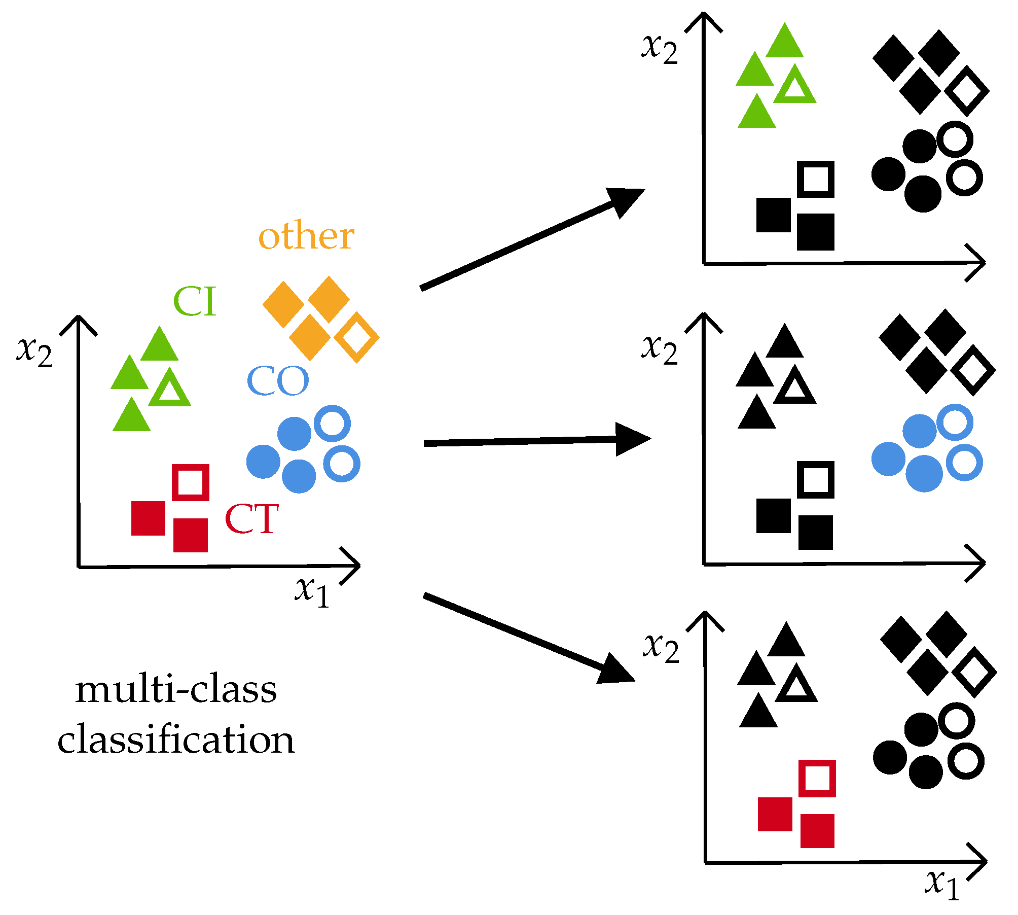
To apply the usual classification quality metrics to this multi-class classification problem, a transformation is needed that decomposes it into several binary tasks. The simplest approach is the One-vs-all (OVA) transformation shown in Figure 11. It generates three binary problems for the three classes, , where each problem discriminates a selected class from the other three classes, including [22]. The resulting binary classification then only distinguishes two discrete classes, e.g.,
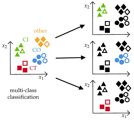
Figure 11.
One-vs-all transformation of multi-class classification problems into binary classification problems (colors and marker types refer to predicted classes, filled markers refer to correct classification, unfilled markers refer to misclassification).

Table 3.
Confusion matrix for cut-in (CI) after OVA transformation.
An ideal classifier would classify all cut-in events as CI and all non-CI maneuvers as non-cut-in. Misclassification occurs when a cut-in maneuver is classified as non-CI, or a non-CI event is classified as CI. These two variants of misclassifications have rather different implications. They are, therefore, distinguished when determining the classification quality.
We can count the following four cases of classification results after the OVA transformation; see Table 3a:
- : number of true-positive outcomes (CI is classified as CI).
- : number of true-negative outcomes (non-CI is classified as non-CI).
- : number of false-positive outcomes (non-CI is classified as CI).
- : number of false-negative outcomes (CI is classified as non-CI).
Based on the absolute frequencies of these four cases, commonly used criteria may be applied. For instance, the accuracy, i.e.,
indicates how well a binary classifier predicts the correct result. According to Table 3, the rule-based decision tree has a lower accuracy of compared to of TSF and, thus, has a lower classification performance.
Regarding problems with several classes, it is important to check the recall and precision of each class. The goal is to achieve maximum recall and precision for each label, which directly results in high accuracy. Recall is the probability that a real event is classified correctly, whereas precision describes the probability that the prediction of an event is correct. In other words, high precision means that the identified scenarios are likely to belong to the corresponding class, whereas high recall means that a large proportion of the real scenarios is identified.
The results of the rule-based decision tree (DT) and time series forest (TSF) for all three scenario types are listed in Table 4. Additionally, the supervised TSF (sTSF) was investigated, which is an extension of TSF, where feature intervals are not randomly selected from the entire time series but are instead determined based on their discriminative ability, enhancing the efficiency of TSF [23]. Moreover, additional features such as median, minimum, maximum, and interquartile range were extracted. All three classification approaches demonstrate high precision and recall performances for all three scenarios. In contrast to the impression gained from the discussion in Section 3, the slight differences confirm that TSF outperforms the other two classifiers. Notably, its highly sensitive approach results in outstanding precision, and its robustness—bolstered by a large number of decision trees with significant depth —yields almost the best recall values for all scenario types.

Table 4.
Precision and recall of various classification methods.
Finally, an overall measure summarizing all three scenarios will be computed. Thereby, it typically should be taken into account that, due to the different rates of occurrence of the different scenario classes, the evaluated dataset is imbalanced. However, because of their equal relevance for risk assessment, here, each scenario class is taken into account equally to define total precision and total recall as arithmetic means
This ultimately results in Table 5, highlighting that over all scenarios, the TSF outperforms the two other classification methods.

Table 5.
Total precision and recall for various classification methods.
6. Conclusions
Validating highly automated driver assistance systems requires accurate risk assessment of safety-relevant driving situations. Detecting and classifying such scenarios in large datasets of measurements is a crucial initial step in the validation process. The currently applied rule-based scenario classification fails to meet all quality needs and is therefore replaced here by a time series forest (TSF) approach, which achieves better classification results. Due to its use of lateral distances to all neighboring vehicles, the TSF approach misses fewer critical scenarios than the rule-based decision tree, which only looks ahead along the ego-driving tube. It is also more robust against misclassifications of non-critical scenarios, thus leading to more reliable predictions of failure probabilities. It should be emphasized that highly idealized samples have been used for training the machine learning model. To further improve its robustness, measured snippets of more realistic artificial maneuvers generated by [15] may be used instead. Additionally, features may be extracted from and combined with the -features already used in the paper.
7. Patents
A patent application is in the preliminary examination.
Author Contributions
Methodology and paper writing, Z.K. and D.B.; software and investigation, Z.K.; supervision, D.B. All authors have read and agreed to the published version of the manuscript.
Funding
The second author is funded by the Deutsche Forschungsgemeinschaft (DFG, German Research Foundation), project no. 501840485.
Data Availability Statement
The datasets presented in this article are not available due to the privacy restrictions of the OEM. Requests to access the datasets should be directed to correspondence.
Conflicts of Interest
The authors declare no conflicts of interest.
References
- Europäisches Parlament. Safer Roads: New EU Measures to Reduce Car Accidents. Available online: https://www.europarl.europa.eu/topics/en/article/20190307STO30715/safer-roads-new-eu-measures-to-reduce-car-accidents (accessed on 7 August 2024).
- Society of Automotive Engineers. Taxonomy and Definitions for Terms Related to Driving Automation Systems for On-Road Motor Vehicles; ISO, J3016_202104; SAE International: Warrendale, PA, USA, 2021. [Google Scholar]
- van der Aalst, W. Six Levels of Autonomous Process Execution Management. arXiv 2022, arXiv:2204.11328. [Google Scholar]
- Richter, A.; Walz, T.P.; Dhanani, M.; Häring, I.; Vogelbacher, G.; Höflinger, F.; Finger, J.; Stolz, A. Components and their Failure Rates in Autonomous Driving. In Proceedings of the 33rd European Safety and Reliability Conference (ESREL 2023), Southampton, UK, 3–7 September 2023. [Google Scholar]
- Goodfellow, I.; Bengio, Y.; Courville, A. Deep Learning; MIT Press: Cambridge, MA, USA, 2016. [Google Scholar]
- Reichenbächer, C.; Rasch, M.; Kayatas, Z.; Wirthmueller, F.; Hipp, J.; Dang, T.; Bringmann, O. Identifying Scenarios in Field Data to Enable Validation of Highly Automated Driving Systems. In Proceedings of the 8th International Conference on Vehicle Technology and Intelligent Transport Systems-VEHITS, Online, 27–29 April 2022; SciTePress: Setúbal, Portugal, 2022; pp. 134–142, ISBN 978-989-758-573-9, ISSN 2184-495X. [Google Scholar] [CrossRef]
- Wagner, J.; Häring, J. Validierung von hochautomatisierten Fahrfunktionen mit cloud-basierter Simulation. ATZ 2020, 122, 50–55. [Google Scholar] [CrossRef]
- Pfeffer, R.; He, J.; Sax, E. Development and implementation of a concept for the meta description of highway driving scenarios with focus on interactions of road users. In Proceedings of the 6th International Conference on Vehicle Technology and Intelligent Transport Systems–VEHITS, Prag, Czech Republic, 2–4 May 2020. [Google Scholar]
- Bock, J.; Krajewski, R.; Eckstein, L.; Klimke, J.; Sauerbier, J.; Zlocki, A. Data Basis for Scenario-Based Validation of HAD on Highways. In Proceedings of the 27th Aachen Colloquium Automobile and Engine Technology, Aachen, Germany, 8–10 October 2018. [Google Scholar]
- PEGASUS. 2019. Available online: https://www.pegasusprojekt.de/en/pegasus-method (accessed on 14 April 2024).
- Muslim, H.; Endo, S.; Imanaga, H.; Kitajima, S.; Uchida, N.; Kitahara, E.; Ozawa, K.; Sato, H.; Nakamura, H. Cut-Out Scenario Generation with Reasonability Foreseeable Parameter Range from Real Highway Dataset for Autonomous Vehicle Assessment. IEEE Access 2023, 11, 45349–45363. [Google Scholar] [CrossRef]
- Zlocki, A.; König, A.; Bock, J.; Weber, H.; Muslim, H.; Nakamura, H.; Watanabe, S.; Antona-Makoshi, J.; Taniguchi, S. Logical Scenarios Parameterization for Automated Vehicle Safety Assessment: Comparison of Deceleration and Cut-In Scenarios from Japanese and German Highways. IEEE Access 2022, 10, 26817–26829. [Google Scholar] [CrossRef]
- Ma, X.; Ma, Z.; Zhu, X.; Cao, J.; Yu, F. Driver Behavior Classification under Cut-In Scenarios Using Support Vector Machine Based on Naturalistic Driving Data; SAE Technical Paper 2019-01-0136; SAE: Warrendale, PA, USA, 2019. [Google Scholar] [CrossRef]
- De Gelder, E.; Paardekooper, J.P.; Saberi, A.K.; Elrofai, H.; den Camp, O.O.; Kraines, S.; Ploeg, J.; De Schutter, B. Towards an Ontology for Scenario Definition for the Assessment of Automated Vehicles: An Object-Oriented Framework. IEEE Trans. Intell. Veh. 2022, 7, 300–314. [Google Scholar] [CrossRef]
- Kayatas, Z.; Bestle, D.; Bestle, P.; Reick, R. Generation of Realistic Cut-in Maneuvers to Support Safety Assessment of Advanced Driver Assistance Systems. Appl. Mech. 2023, 4, 1066–1077. [Google Scholar] [CrossRef]
- Pirouz, A. Identifizierung Kritischer Fahrszenarien aus Messdaten Mittels Machine Learning Methoden. Master’s Thesis, University of Stuttgart, Stuttgart, Germany, 2021. [Google Scholar]
- Deng, H.; Runger, G.; Tuv, E.; Vladimir, M. A Time Series Forest for Classification and Feature Extraction. Inf. Sci. 2013, 239, 142–153. [Google Scholar] [CrossRef]
- Roesener, C.; Harth, M.; Weber, H.; Josten, J.; Eckstein, L. Modelling Human Driver Performance for Safety Assessment of Road Vehicle Automation. In Proceedings of the 21st International Conference on Intelligent Transportation Systems (ITSC), Maui, HI, USA, 4–7 November 2018. [Google Scholar] [CrossRef]
- De Gelder, E.; Hof, J.; Cator, E.; Paardekooper, J.P.; den Camp, O.O.; Ploeg, J.; De Schutter, B. Scenario Parameter Generation Method and Scenario Representativeness Metric for Scenario-Based Assessment of Automated Vehicles. IEEE Trans. Intell. Transp. Syst. 2022, 23, 18794–18807. [Google Scholar] [CrossRef]
- Storn, R.; Price, K. Differential Evolution—A Simple and Efficient Heuristic for Global Optimization over Continuous Spaces. J. Glob. Optim. 1997, 11, 341–359. [Google Scholar] [CrossRef]
- Fletcher, R. Methods of Optimization; Wiley: Chichester, UK, 1987. [Google Scholar]
- Rifkin, R.; Klautau, A. In Defense of One-vs-All Classification. J. Mach. Learn. Res. 2004, 5, 101–141. [Google Scholar]
- Cabello, N.; Naghizade, E.; Qi, J.; Kulik, L. Fast and Accurate Time Series Classification through Supervised Interval Search. In Proceedings of the IEEE International Conference on Data Mining, Sorrento, Italy, 17–20 November 2020. [Google Scholar] [CrossRef]
Disclaimer/Publisher’s Note: The statements, opinions and data contained in all publications are solely those of the individual author(s) and contributor(s) and not of MDPI and/or the editor(s). MDPI and/or the editor(s) disclaim responsibility for any injury to people or property resulting from any ideas, methods, instructions or products referred to in the content. |
© 2024 by the authors. Licensee MDPI, Basel, Switzerland. This article is an open access article distributed under the terms and conditions of the Creative Commons Attribution (CC BY) license (https://creativecommons.org/licenses/by/4.0/).

