Non-Linear Model of Predictive Control-Based Slip Control ABS Including Tyre Tread Thermal Dynamics

Abstract

Vehicle dynamics can be deeply affected by various tyre operating conditions, including thermodynamic and wear effects. Indeed, tyre temperature plays a fundamental role in high performance applications due to the dependencies of the cornering stiffness and potential grip in such conditions. This work is focused on the evaluation of a potentially improved control strategy’s performance when the control model is fed by instantaneously varying tyre parameters, taking into account the continuously evolving external surface temperature and the vehicle boundary conditions. To this end, a simplified tyre thermal model has been integrated into a model predictive control strategy in order to exploit the thermal dynamics’ dependents within a proposed advanced ABS control system. We evaluate its performance in terms of the resulting braking distance. In particular, a non-linear model predictive control (NMPC) based ABS controller with tyre thermal knowledge has been integrated. The chosen topic can possibly lay a foundation for future research into autonomous control where the detailing of decision-making of the controllers will reach the level of multi-physical phenomena concerning the tyre–road interaction.

1. Introduction

Tyres play an important role in vehicle dynamics modelling and control, as they allow the vehicle’s interaction with the road. The vehicle’s dynamic performance may vary considerably depending on the road and tyre characteristics (inner pressure, ageing, and temperature), which can affect tyre friction and stiffness due to multi-material interactions and viscoelastic rubber matrix compositions [1,2,3,4].

The widely accepted systems such as the Anti-lock Braking System (ABS), Traction Control (TC), and Electronic Stability Control (ESC) may still perform sub-optimally without considering the tyres’ multi-physical phenomena (temperature, wear, etc.) [5,6,7,8,9]. A vehicle dynamics control system that either does not control tyre temperature or only regulates the tyre temperature will not be able to ensure adequate vehicle performance. Such systems could potentially be modified by incorporating tyre states (especially temperature) to improve their performance [10,11,12].

This paper investigates whether the proposed model-based optimal controller will be able to improve the overall performance of the system considering the tyre thermodynamics and its influence on adherence and stiffness quantities in the controller model. To this end, an ABS was chosen as the target system in this work, adopted as a preliminary application making use of the tyres’ longitudinal interaction, but nevertheless it constitutes an necessary foundation for further studies making use of vehicle yaw-rate regulators or full autonomous controllers, such as that presented by Sakhnevych [13]. In particular, this study includes the thermodynamic variation and its influence on the global dynamics of the vehicle directly within the control logic, trying to understand how an optimal control logic should be designed to govern both thermal and non-linear dynamic behaviour of the system in all possible boundary conditions of interest, identified by the ambient asphalt and air temperatures. To examine the potential of giving the controller the knowledge of tyre temperature on the performance of ABS, a non-linear model predictive control-based slip control ABS was developed and tested on a full-car plant model within a simulation environment. The main objective of ABS is to maximise the braking performance, quantified by braking distance, and at the same time, to guarantee the vehicle’s steering ability. This objective can be synthesised as the controller system keeping the longitudinal slip value around the point corresponding to the maximum longitudinal force. In a braking manoeuvre, the tyre heats up inevitably, affecting both the slip stiffness and the peak grip. The knowledge of the peak grip will help the controller make better decisions of control input, i.e., brake torque. The information concerning the vehicle’s non-linear physical limits, in their turn depending on the instantaneous thermal states of tyres and on the boundary conditions (in terms of air and track temperatures), can be of great additional value for the optimal behaviour of a safety- and performance-oriented control strategy. Therefore, advanced driving systems should become adaptive due a continuous physically-based evaluation of adherence, sensitive to environmental conditions, and possibly by employing scientifically reliable model-based fusion methodologies.

The remainder of the paper is organised as follows: Section 2 describes the overall methodology, including the tyre and vehicle models used. Section 3 presents the results obtained from the developed tyre and full-car model compared to the validated full-car VI CarRealTime from the VI-grade GmbH model and RIDEsuite tyre model results. In Section 4 the controller description is presented described. In Section 5 the test and metrics adopted to evaluate the control strategy’s performance are presented. Section 6 shows the results, and the discussion is presented in Section 7.

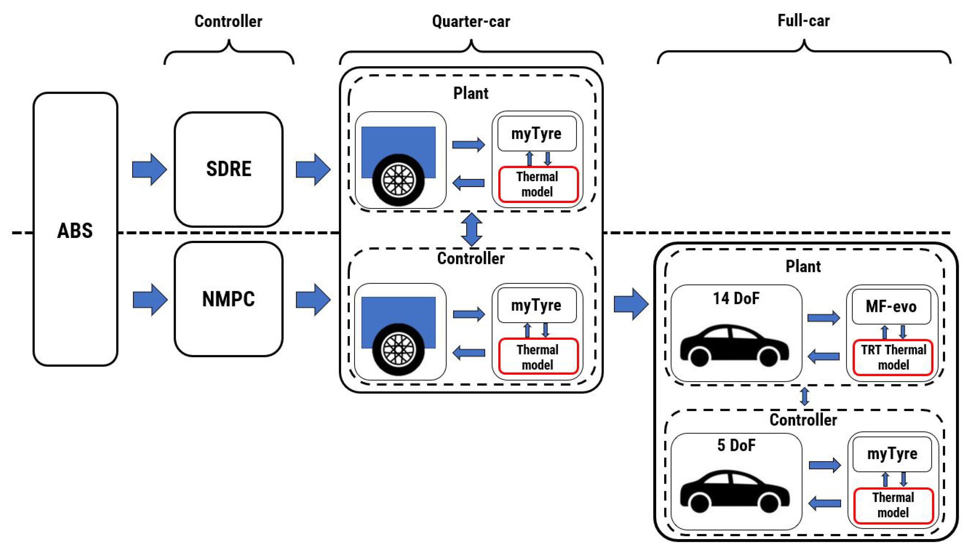
2. Methodology and Co-Simulation Platform

Modern computer technology has enabled us to solve complex non-linear problems numerically in finite time with great accuracy; nowadays, it is very common for organisations to develop digital twins of products for prototyping. This approach has great benefits in the fact that testing variations are virtually infinite as compared to real world testing. Hence, products can be developed quickly while being cost-effective. Of course, the former statement is only true if the plant models being used are validated. However, such an approach at least helps cut down a lot of possibilities that would have been tested in real-life prototypes with no fruitful results.

Such a method is especially great for research studies where an exploration of the proposed idea is to be checked or the focus is at least not to develop the whole product but just the concept.

As the application is concerned with vehicle control related to tyre performance, existing control systems such as ABS and ESC instantly come to mind. ABS in particular was chosen to be developed and tested. The focus was kept on high-level control and not the detailing of the low level hydraulic braking system, i.e., the actuator dynamics.

Concerning the optimal controllers, as stated in the literature survey, SDRE and NMPC were the two chosen options to test. Figure 1 shows the approach taken for the whole ABS development process. For each controller, first the quarter-car approach was used. In this system, the plant was modelled the same as the prediction model used inside the controllers.

After the quarter-car development, the full-car controller was developed only for the NMPC-based controller, as the SDRE controller did not provide much opportunity for tuning and was very unstable at lower velocities. It was performed using the co-simulation in a Simulink environment. The full-car model has 14 degrees of freedom (DoF), based on the mathematical representation described in [14], and has been modelled in a MATLAB/Simulink environment as follows:

• Six DoF to reproduce longitudinal, lateral, vertical, pitch, roll, and yaw motion of the vehicle body;
• Four DoF concerning the wheel rotation and four DoF for the wheel normal displacement, with the hypothesis that the degrees of freedom relative to the motion between the wheel and the vehicle body can be neglected along the longitudinal and lateral directions, allowing only the independent rotational and vertical displacements.

Furthermore, the parameterised vehicle is rear-wheel drive with front steering and internal combustion engine. The tyre model is described by Pacejka’s magic formula evolved model and is coupled with the validated high-fidelity multi-physical tyre described in Section 2.1 and thermal model described in [15] called ’TRT: Thermo Racing Tyre’, whereas the prediction model inside the controller includes a 5-DOF vehicle longitudinal model (Section 2.3.2) coupled with the same myTyre as used in the case of the quarter-car. The whole controller was modelled in Simulink, and Simulink was the environment for the simulations with the full-car model.

2.1. Tyre Model

This section explains the tyre model developed for the prediction model inside the optimal controllers. It has been named ’myTyre’ so that the reader can easily understand and pinpoint its exact usage. This model is a combination of the basic equations of the Pacejka tyre model [16] and the tyre tread thermal model used to alter the stiffness and the peak force of the Pacejka equations. The literature showed that using a steady-state tyre model (for the optimal controller predictions) should be good for ABS simulations, and thus no transient effects (such as relaxation length for the longitudinal force) were modelled. The following paragraphs explain the details of the Pacejka force model, the thermal model, and the connection between the two, as shown in Figure 2.

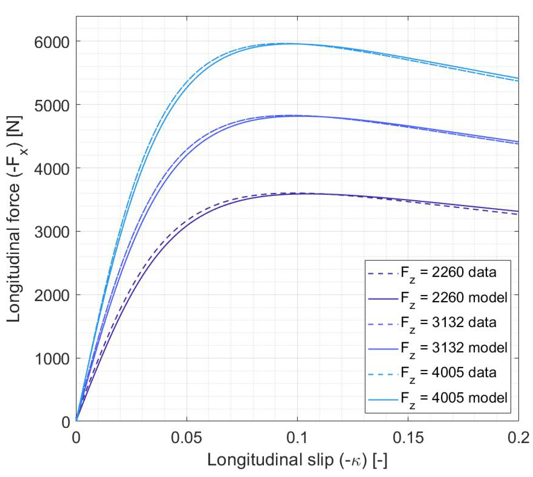
Tyre Force Model—Pacejka Model Based

The most famous empirical tyre model equation, the Pacejka MF tyre model [16], has been used to represent the longitudinal tyre forces. It has been used in innumerable applications since its inception in 1990s. Based on the similarities concept, each parameter inside the equation is related to different characteristics of the tyre, such as peak force and stiffness. Additionally, the dependencies of these parameters can be made functions of the desired variable—for example, the tyre’s normal load. For high-level ABS controller testing, longitudinal tyre modelling is sufficient, especially for longitudinal tests where no lateral tyre slip is encountered. In this study, the focus is only kept on the performance of ABS in straight-line tests with the same coefficient of friction for all the tyres; hence, a pure longitudinal model is sufficient. In the case of brake test cases involving cornering or split-$\mu$ conditions, the use of a combined slip–tyre equation is crucial.

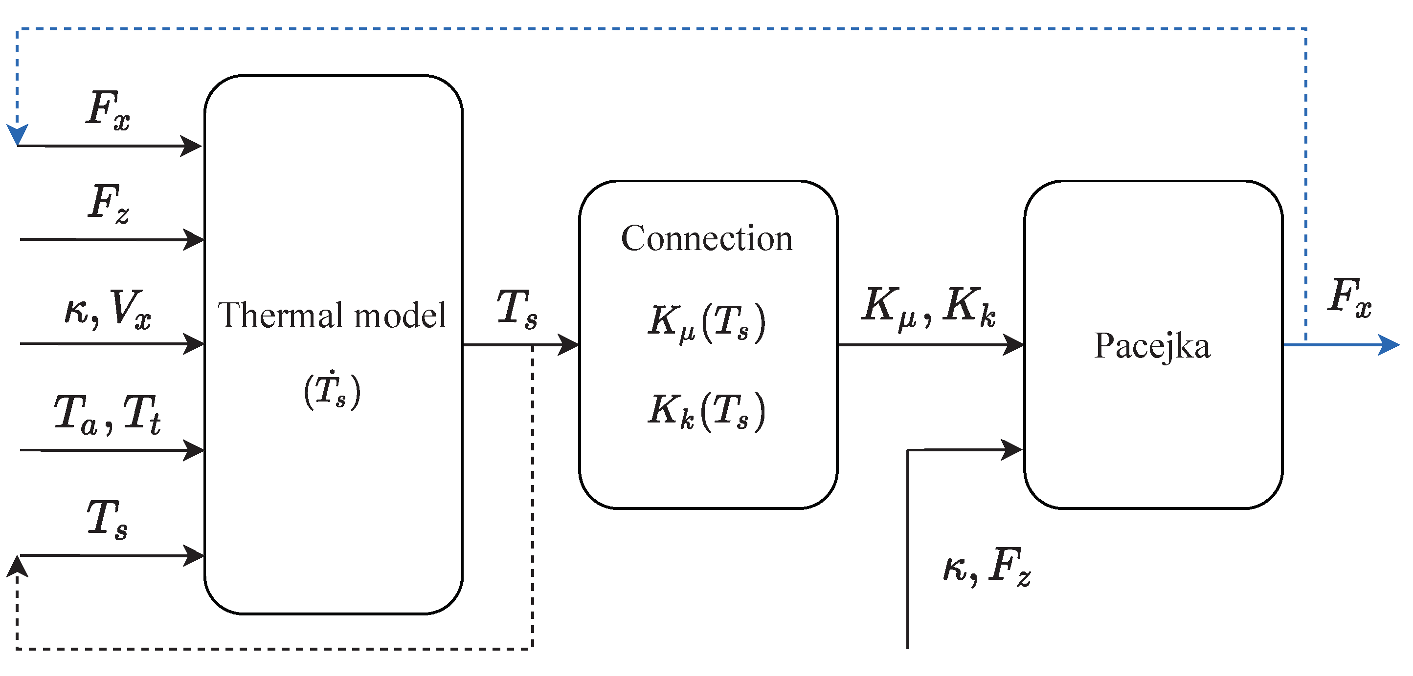
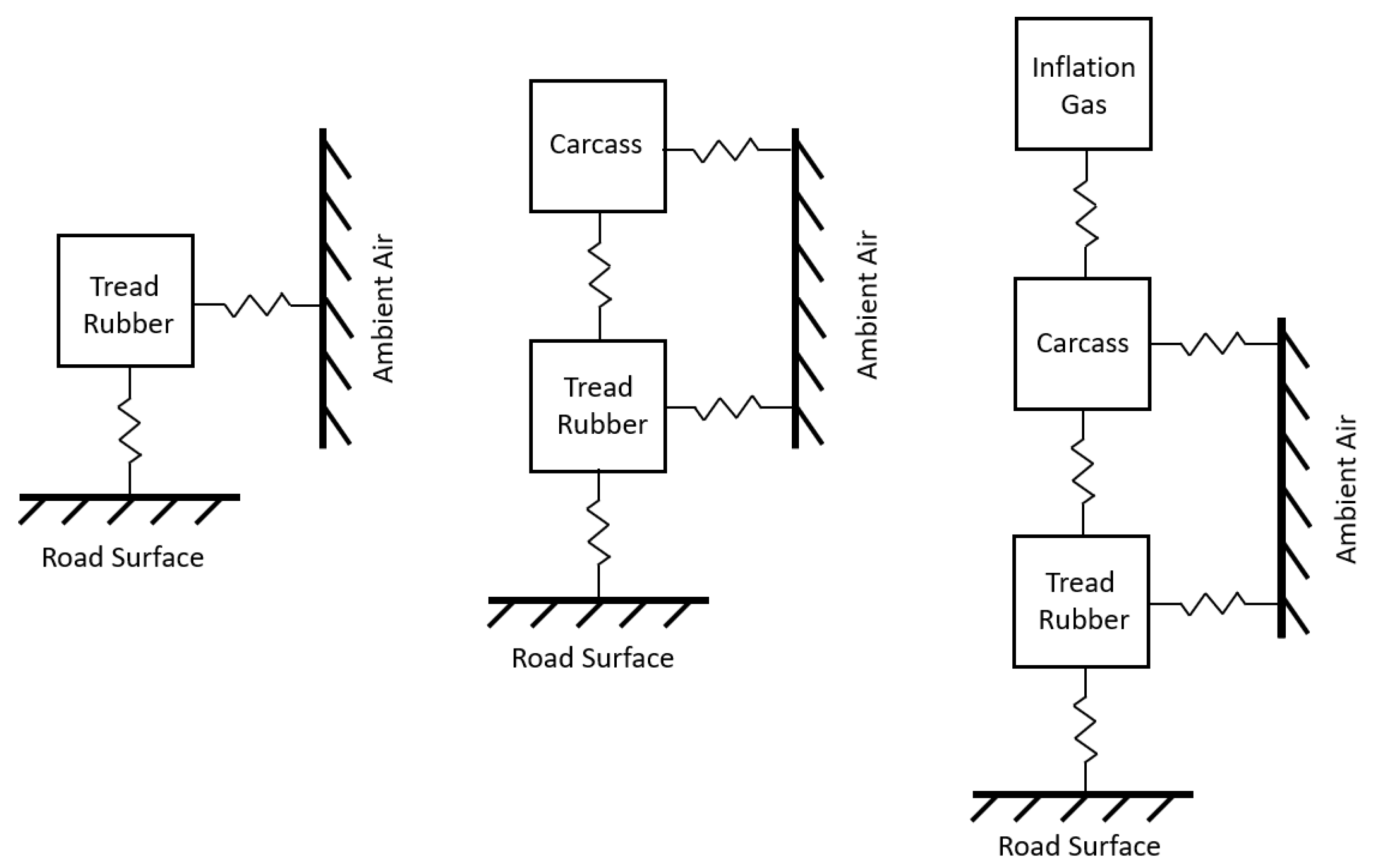
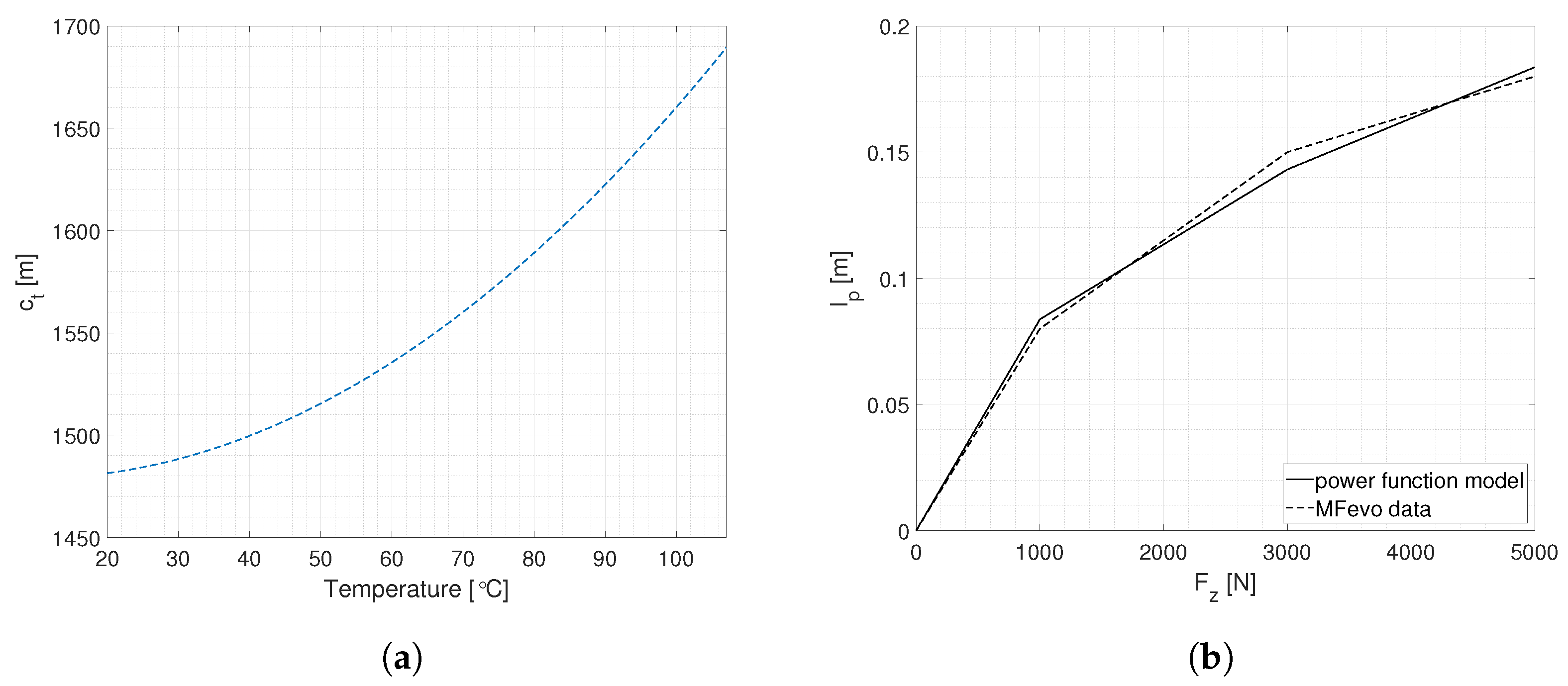
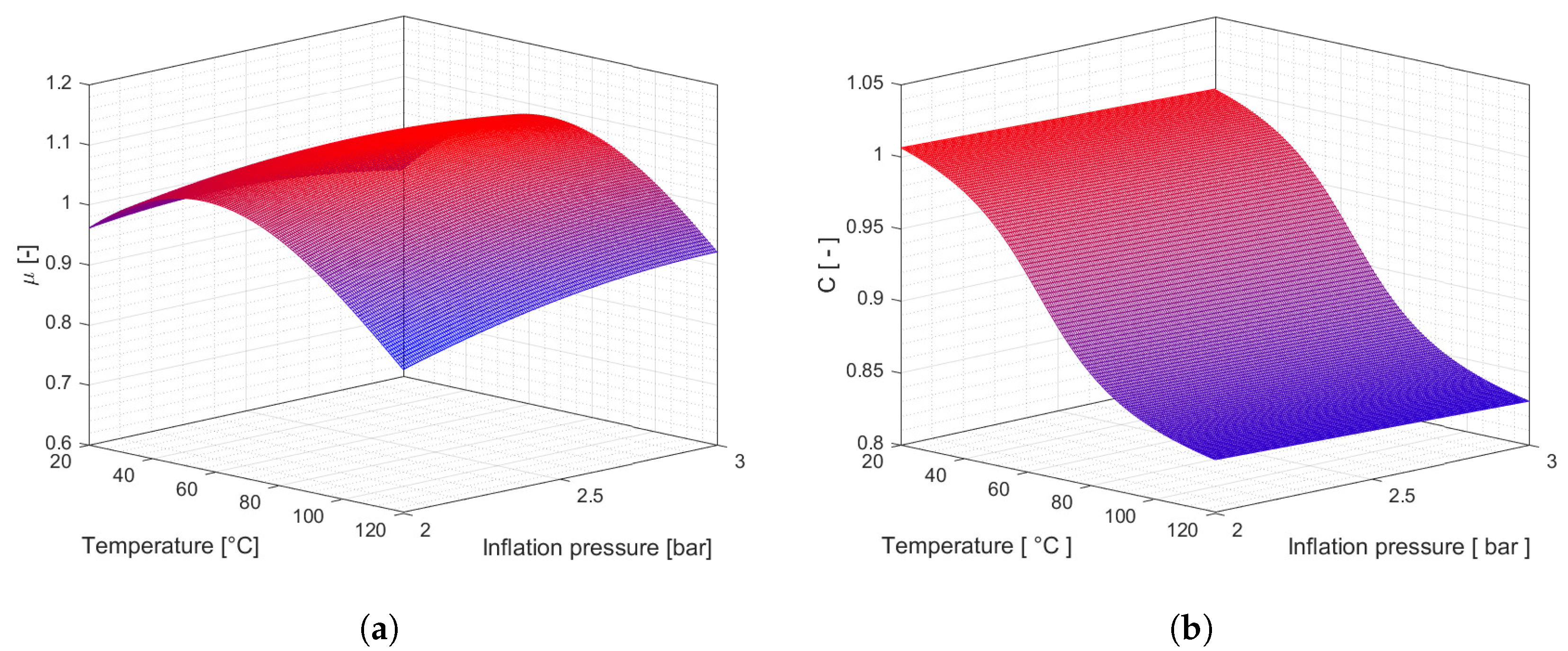
2.2. Tyre Thermal Modelling

Much of the literature on tyre thermal modelling is related to the accuracy provided in the simulations in model-based development of vehicles [17,18,19,20,21,22]. These models range from simple empirical-lumped models to high-fidelity finite element method(FEM)-based physical models. Additionally, because modern development also involves driver in the (DiL) simulations, the numerical solutions of such models must also converge in real-time based on the current state-of-the-art financially viable computer technology. In the following paragraphs, the applicability of the aforementioned models is discussed.

A purely physical model with a 3D FEM-based thermal and structural tyre model was presented by Calabrese [23], with major heat generation and heat exchange sources clearly pointed out. He also presented a setup with a force model based on the MF-tyre model with empirical relations for the grip’s dependency and stiffness’s dependency on the temperature. As pointed out by the author, the latter setup has a lower computational cost. Regardless, both setups shows high accuracy and have great applications for lap-time simulations or tyre development, due to using a physical model. Unquestionably, such a model cannot be considered for the prediction model inside an optimal-controller, being computationally heavy, as it involves solving partial differential equations in three dimensions.

The physical model (1D-heatflow) presented by Rosa et al. [24] set the foundations for the 3D physical model later presented by Farroni et al. [1,25] for motorsport applications ’to estimate the temperature distribution even of the deepest tyre layers’. As stated by the authors, these models have shown great real-time applicability for DiL simulations. However, the same reasoning as for the Calabrese’s model [23] goes for it being inappropriate as a prediction model for a controller.

The model presented by Tremlett [21] is a great example of a lumped-parameter model based on the heat flow equation formed using the first law of thermodynamics with the assumption of an isotropic thermal tyre mass. They treat the tread of the tyre as a lumped mass with four dominant heat-flows, viz., friction power, strain energy, air convection, and conduction in the non-sliding region of the patch. These individual heat flow terms are fit empirically with their individual efficiency terms. The model involves a solution of a single ordinary differential equation (ODE) to predict the tread temperature, which makes it suitable for a prediction model inside an optimal controller, unlike a 3D model solved using FEM. As shown in Figure 3, a similarly lumped, 2-node (tread and carcass) thermal model by West and Limebeer [22], and a 3-node (tread, carcass, and internal air) thermal model by Kelly and Sharp [6] can possibly accommodate bigger variations in boundary conditions as compared to the aforementioned 1-node (tread) model. Thus, they could also be used in future applications and have the advantage of robustness.

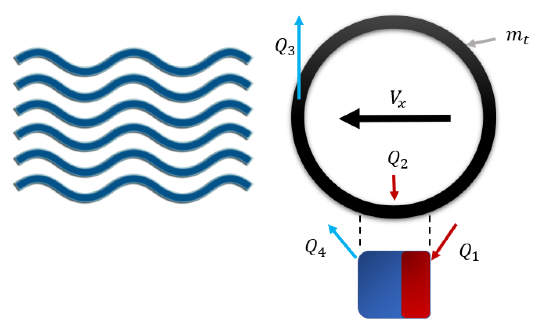
2.2.1. Thermal Model

As was discussed in the literature survey, the thermal model developed by Tremlett [21] with some modifications related to the contact-patch-size-related functions according to Hackl [19] was implemented.

The model in focus is an empirical lumped-parameter model of the tyre tread based on the first law of thermodynamics. The tread mass is treated as an isotropic material. This tyre tread (1-node) model was an obvious starting point for this problem, not just owing to the need for a light and simple model, but also due to the fact that the employed model-based controllers need full-state feedback. The tread temperature is known to be easily measured with the use of infrared sensors in modern cars, whereas in the case of a 2-node model with the additional temperature state of the carcass temperature, state estimation techniques would be necessary for the requirement of full-state feedback.

The following four heat flows (Figure 4), being the dominant one, are considered, while radiation is neglected:

• $Q_1$: Heat generated due to the friction power in the sliding region of the contact patch;
• $Q_2$: Heat generated due to the strain energy within the mass;
• $Q_3$: Heat exchange due to the forced convection with ambient air;
• $Q_4$: Heat exchange due to the conductive cooling in the non-sliding region of the contact patch.

The homogeneous temperature of the tread mass ($T_s$) is given by the differential equation:

$$m_t{c}_t{\dot{T}}_s=Q_1+Q_2-Q_3-Q_4$$

(1)

where $m_t$ is the mass of the tyre tread and $c_t$ its specific heat capacity. The heat generation due to friction power ($Q_1$) is represented as a sum of friction powers due to $F_x$ (2), and the same heat due to $F_y$ is neglected, as we are using the pure longitudinal representation:

$$Q_1=p_1{V}_x\left|F_x\kappa \right|$$

(2)

where $V_x$ is the tyre ground velocity and $p_1$ represents the ratio of friction heat entering the tread. All the parameters (viz., $p_i$) in this model are fit empirically. The heat generation due to strain energy ($Q_2$) is represented as shown in Equation (3); the parameters here are the efficiencies related to each force, i.e., $F_x$ and $F_z$ in this case. These efficiencies directly relate to the corresponding forces’ contributions to the strain energy losses:

$$Q_2=V_x(p_2|F_x|+p_3|F_z\left|\right)$$

(3)

Next, the heat exchange due to forced convection around the tyre ($Q_3$) with the ambient air is represented using Newton’s cooling law with an empirical formulation for the heat transfer coefficient, as seen in Equation (4):

$$Q_3=p_4{V}_x^{p_5}(T_s-T_{amb})$$

(4)

where $T_{amb}$ is the ambient temperature and the heat coefficient is represented as $p_4{V}_x^{p_5}$ and is empirically fit. The formulation $p_4{V}_x^{p_5}$ can very well represent the flow around a wheel in a car, once fit. Lastly, the heat exchange due to the conduction of the non-sliding region of the patch ($Q_4$) with the road is represented using Fourier’s law, as shown in Equations (5)–(9):

$$Q_4=h_t{A}_{nsl}(T_s-T_{road})$$

(5)

where,

$$A_{nsl}=l_w{l}_{nsl}$$

(6)

$$l_{nsl}=l_p(1-c_s)$$

(7)

$$l_p=a_{cp}{F}_z^{a_{cpp}}$$

(8)

$$c_s=\left(\frac{c_{s2}-c_{s1}}{{\kappa }_{max}}\right)\kappa +c_{s1}$$

(9)

For the non-sliding region area calculation, the whole patch is assumed as a rectangle with length $l_p$ and width $l_w$; and it was a safe choice to assume that the width remains fixed (being a radial tyre). The $l_w$ is represented as a power function of the tyre normal load, as shown in Equation (8), fit empirically using separate data. The non-sliding region’s length $l_{nsl}$ is calculated by first knowing the sliding length $l_{sl}$ of the patch using the proportioning factor $c_s$, as shown in Equations (7) and (9). $c_s$ is a linear function of the longitudinal slip based on the values proposed by Hackl [19]. Here, $c_{s2}$ and $c_{s1}$ are the proportions of the patch region that are sliding with the slip value at maximum force (${\kappa }_{max}$) and zero slip, respectively. Additionally, the heat transfer coefficient $h_t$ is taken as a constant.

2.2.2. Connection $K_{\mu }\left(T_s\right)$ and $K_k\left(T_s\right)$

As seen in Calabrese’s work [23], the two main effects that the tyre temperature has on the tyre characteristics are on grip and stiffness; grip experiences a considerable change. However, in high-fidelity models such as MFevo, the grip and stiffness changes are more precisely represented as functions of different internal tyre layer temperatures and also pressure, as shown in [13,26]. In myTyre, the grip and slip stiffness effect were included using the $K_{\mu }\left(T_s\right)$ and $K_k\left(T_s\right)$ functions by scaling $D_x$ and $B_x$, respectively. These scaling functions are shown in Equation (10). Their polynomial degrees were based on the identification of the data from the reference tyre at a given pressure. It is safe to assume the pressure as constant for a given manoeuvre, but across the whole working range of environmental conditions, in reality it is crucial to consider the pressure effect. In all the tests performed in this work, the initial pressure was assumed to be the same ($1.4bar$), no matter the environmental conditions.

Although the cornering stiffness of the tyre is more dependent on the carcass temperature than the tread temperature, because of some amount of correlation, a cubic polynomial (10) shows a good enough empirical fit, at least in terms of the direction of trend:

$$K_{\mu }=K_{\mu ,a}{T}_s^2+K_{\mu ,b}{T}_s+K_{\mu ,c}$$

(10a)

$$K_{\mu }=K_{k,a}{T}_s^3+K_{k,b}{T}_s^2+K_{k,c}{T}_s+K_{k,d}$$

(10b)

where $K_{mu,i}$ and $K_{k,i}$ are the coefficients of respective polynomials ($i\in \{a,b,c,d\}$ here).

2.3. Vehicle Model

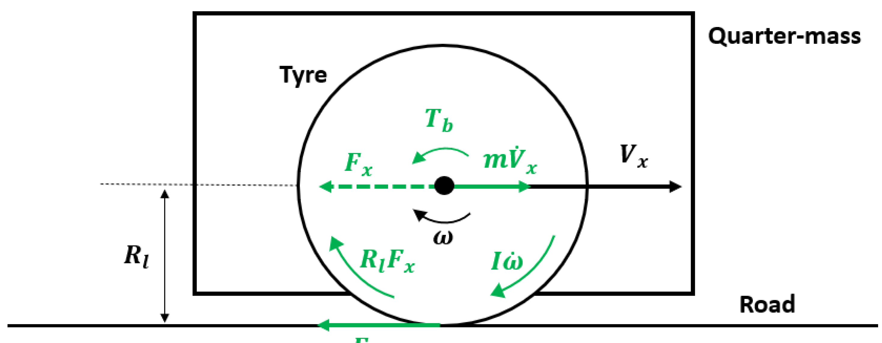
2.3.1. Quarter-Car

A quarter-car is a model representing one corner of a car which includes the equivalent mass at that corner and the wheel. This leads to three main dynamics to be modelled, viz., wheel slip dynamics, longitudinal velocity of the quarter-car, and the tread temperature dynamics. No load transfer effect (no moment balance) is considered due to the fact that there is only one tyre. Figure 5 shows us a quarter-car where only the longitudinal force balance between inertial force and tyre force, and the torque balance among inertial torque, brake torque, and tyre force torque, are taken into account. Additionally, the tyre normal load is simply equal to the weight of the quarter-car (mg).

Such a simple model helps us understand the basics of the full-vehicle and also use better weight tuning for the full-car controller. This model, coupled with myTyre, was both used as the plant and prediction model. The following points state the assumptions after simplification:

• It moves in a straight line, and thus, longitudinal dynamics of tyre must suffice;
• No camber ($\gamma$) effects;
• No suspension/load transfer effects considered;
• Purely rigid longitudinal connections;
• No coupling effects due to a chassis connecting the four wheels;
• No variations in wheel radius.

From the longitudinal slip definition in equation:

$$\left\{\begin{array}{c}{s}_x=\frac{V-\mathsf{\Omega }\times R}{V_x}\hfill \\ s_y=\frac{V_y}{V_x}=tan\alpha \approx \alpha \hfill \end{array}\right.$$

(11)

it was possible get the following Equation (12).

$$\dot{\kappa }=\frac{1}{V_x}\left[R_e\dot{\omega }-{\dot{V}}_x\left(1+\kappa \right)\right]$$

(12)

By balancing the torque around the wheel centre, the wheel rotation dynamics ($\dot{\omega }$) have been evaluated as (13):

$$\dot{\omega }=\frac{T_b-R_l{F}_x}{I}$$

(13)

where $T_b$ is the braking torque applied to the wheel, $R_l$ is the loaded radius of the tyre, $F_x$ is the longitudinal tyre force, and I is the wheel’s total rotational inertia about the rotation axis.

A simple longitudinal equilibrium on the quarter-car brings us Equation (14):

$${\dot{V}}_x=\frac{F_x}{m}$$

(14)

where m is the mass of the quarter-car.

By substituting the values of $\dot{\omega }$ from Equation (13) and ${\dot{V}}_x$ from Equation (14) into Equation (12), we get the following Equation (15):

$$\dot{\kappa }=\frac{1}{V_x}\left[\frac{R_e{T}_b}{I}-F_x\left(\frac{R_e{R}_l}{I}+\frac{1+\kappa }{m}\right)\right]$$

(15)

In the tyre tests it was also seen that unlike the loaded radius, the effective radius does not change much unless there are larger values than the maximum force. Thus, a constant value was chosen and not modelled as a dependent variable for factors such as tyre load and speed.

Finally, using the tread temperature dynamics definition ${\dot{T}}_s$ from Equation (1), we can get the quarter-car system’s equation in implicit form:

$$\left[\begin{array}{c}\dot{\kappa }-\frac{1}{V_x}\left[\frac{R_e{T}_b}{I}-F_x\left(\frac{R_e{R}_l}{I}+\frac{1+\kappa }{m}\right)\right]\\ {\dot{V}}_x-\frac{F_x}{m}\\ {\dot{T}}_s-\frac{1}{m_t{c}_t}\left(Q_1+Q_2-Q_3-Q_4\right)\end{array}\right]=\left[\begin{array}{c}0\\ 0\\ 0\end{array}\right]$$

(16)

where the heat flows ($Q_i$) are represented as shown in Equations (2)–(5) and have been omitted for spatial reasons. All the $F_x$ terms are represented by the Pacejka tyre force equations.

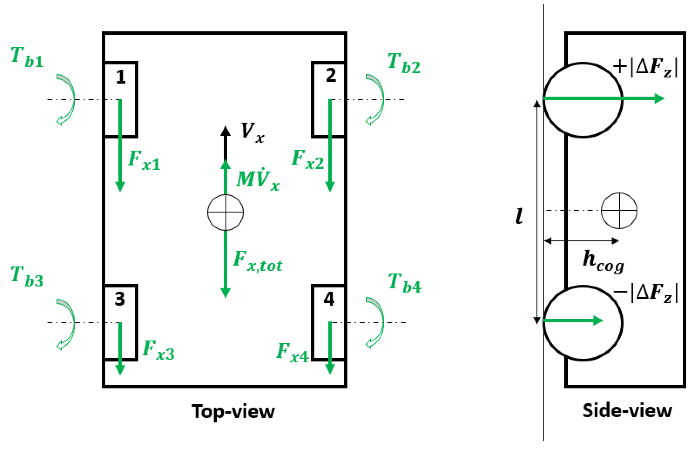
2.3.2. Full-Car

For the full-car analysis, the plant and the prediction models had different fidelities. The plant was the 14-DOF vehicle model based on the mathematical representation described in [14]. It was modelled in a MATLAB/Simulink environment as follows:

• Six DoF to reproduce longitudinal, lateral, vertical, pitch, roll, and yaw motion of the vehicle body;
• Four DoF concerning the wheel rotation and four DoF for the wheel normal displacement, with the hypothesis that the degrees of freedom relative to the motion between the wheel and the vehicle body can be neglected along the longitudinal and lateral directions, allowing only the independent rotational and vertical displacements.

Furthermore, the parameterised vehicle was rear-wheel drive with front steering and internal combustion engine.

The prediction model was a 5-DOF vehicle model used inside the controller.

2.3.3. 5-DOF Vehicle Prediction Model

The prediction model is much simpler than the plant model, and is used to depict the main dynamics of the system important for this controller application, viz., wheel slip dynamics ($\dot{\kappa }$), and the vehicle’s coupled longitudinal dynamics (${\dot{V}}_x$). Our considered reference plant model has four wheels, which corresponds to four slip dynamic equations and a single equation representing the vehicle’s longitudinal dynamics, leading to five degrees of freedom (Figure 6).

Ideally, The load transfer will be included as a function of the vehicle longitudinal acceleration. This acceleration, being a direct function of the tyre force, leads to the situation of an algebraic loop for numerical simulations requiring a special solver which is not a possibility in the case of the Runge–Kutta solver used inside the NMPC prediction calculations. Thus, to avoid the issue an of algebraic loop, the load transfer ($\mathsf{\Delta }{F}_z$) was modelled as first-order dynamics [27], as a function of the tyre longitudinal force, as shown in (17) and (18). Thus, the load transfer was a state in the full-car dynamics, eventually increasing the DOF from 9 to 10, as seen in (20).

$$\dot{\mathsf{\Delta }}{F}_z=\frac{1}{\tau }\left(\tilde{\mathsf{\Delta }}-\mathsf{\Delta }{F}_z\right)$$

(17)

where

$$\tilde{\mathsf{\Delta }}=\frac{F_{x,tot}{h}_{cog}}{2l}$$

(18)

Here, $\tau$ represents the time constant of the first-order transfer function, $h_{cog}$ is the height of the centre of gravity of the whole vehicle, l is the wheelbase, and $F_{x,tot}$ is the summation of all four tyre longitudinal forces. The time constant is fit empirically based on one of the braking tests performed.

Finally, the load transfer is calculated by subtracting or adding the load transfer to the static front/rear wheel loads, respectively, as shown in Equation (19).

$$F_{zi}=F_{z,static}\pm \mathsf{\Delta }{F}_z$$

(19)

The equations for myVeh, including the tyre tread dynamics (additional four degrees of freedom), are presented in implicit form in Equation (20). The index of a variable corresponds to one wheel, as shown in Figure 6.

$$\left[\begin{array}{c}{\dot{\kappa }}_1-\frac{1}{V_x}\left[\left(\frac{R_e}{I}\right)T_{b1}-\left(\frac{R_e{R}_l}{I}\right)F_{x1}-\left(1+{\kappa }_1\right)\frac{F_{x,tot}}{M}\right]\\ {\dot{\kappa }}_2-\frac{1}{V_x}\left[\left(\frac{R_e}{I}\right)T_{b2}-\left(\frac{R_e{R}_l}{I}\right)F_{x2}-\left(1+{\kappa }_2\right)\frac{F_{x,tot}}{M}\right]\\ {\dot{\kappa }}_3-\frac{1}{V_x}\left[\left(\frac{R_e}{I}\right)T_{b3}-\left(\frac{R_e{R}_l}{I}\right)F_{x3}-\left(1+{\kappa }_3\right)\frac{F_{x,tot}}{M}\right]\\ {\dot{\kappa }}_4-\frac{1}{V_x}\left[\left(\frac{R_e}{I}\right)T_{b4}-\left(\frac{R_e{R}_l}{I}\right)F_{x4}-\left(1+{\kappa }_4\right)\frac{F_{x,tot}}{M}\right]\\ {\dot{V}}_x-\frac{F_{x,tot}}{M}\\ {\dot{T}}_{s1}-\frac{1}{m_{t1}{c}_{t1}}\left(Q_{11}+Q_{21}-Q_{31}-Q_{41}\right)\\ {\dot{T}}_{s2}-\frac{1}{m_{t2}{c}_{t2}}\left(Q_{12}+Q_{22}-Q_{32}-Q_{42}\right)\\ {\dot{T}}_{s3}-\frac{1}{m_{t3}{c}_{t3}}\left(Q_{13}+Q_{23}-Q_{33}-Q_{43}\right)\\ {\dot{T}}_{s4}-\frac{1}{m_{t4}{c}_{t4}}\left(Q_{14}+Q_{24}-Q_{34}-Q_{44}\right)\\ \dot{\mathsf{\Delta }}{F}_z-\frac{1}{\tau }\left(\tilde{\mathsf{\Delta }}-\mathsf{\Delta }{F}_z\right)\end{array}\right]=\left[\begin{array}{c}0\\ 0\\ 0\\ 0\\ 0\\ 0\\ 0\\ 0\\ 0\end{array}\right]$$

(20)

where the indices for the variables ${\kappa }_i$, $T_{bi}$, $F_{xi}$, $T_{si}$, $m_{ti}$, $c_{ti}$, and $Q_{ji}$ are defined as $i\in \{1,2,3,4\}$ representing each wheel (Figure 6) and $j\in \{1,2,3,4\}$ representing each heat flow for individual wheel (Equations (2)–(5)). Similarly to the quarter-car, $F_{xi}$ is represented by Pacejka’s tyre force equations. Additionally, the load transfer state equation is represented as shown in Equation (17). M represents the mass of the full-car and $F_{x,tot}$ represents the sum of all $F_{xi}$. It can also be seen that the $R_e$, $R_l$, I, $m_t$, $c_t$, and other thermal parameters are assumed to be the same for all wheels, as all four tyres are represented using the same parameterisation.

3. Validation

This section talks about the parameterisation process used for each model and shows the validation plot for each.

Specifically, the validation of the myVeh tyre model and the myVeh full-car model is shown here. They were fit onto the data obtained from the tests performed with the full-car plant model and the MF-evo tyre with the TRT thermal model.

Finally, the validation of the plant model and MFevo tyre model are described.

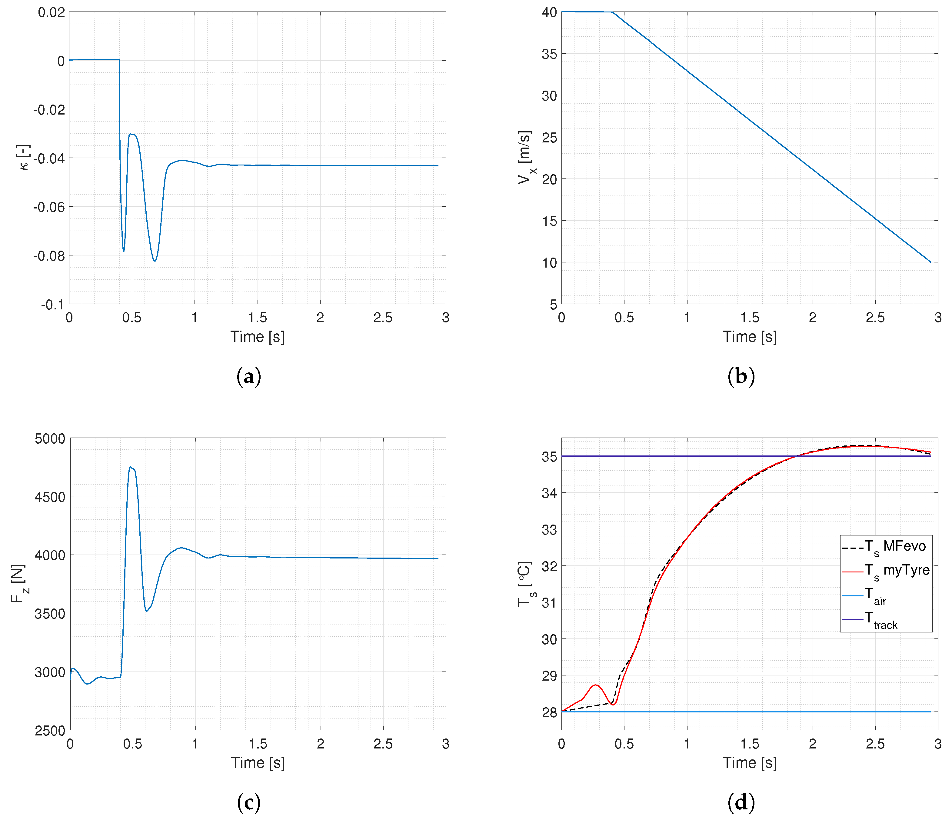
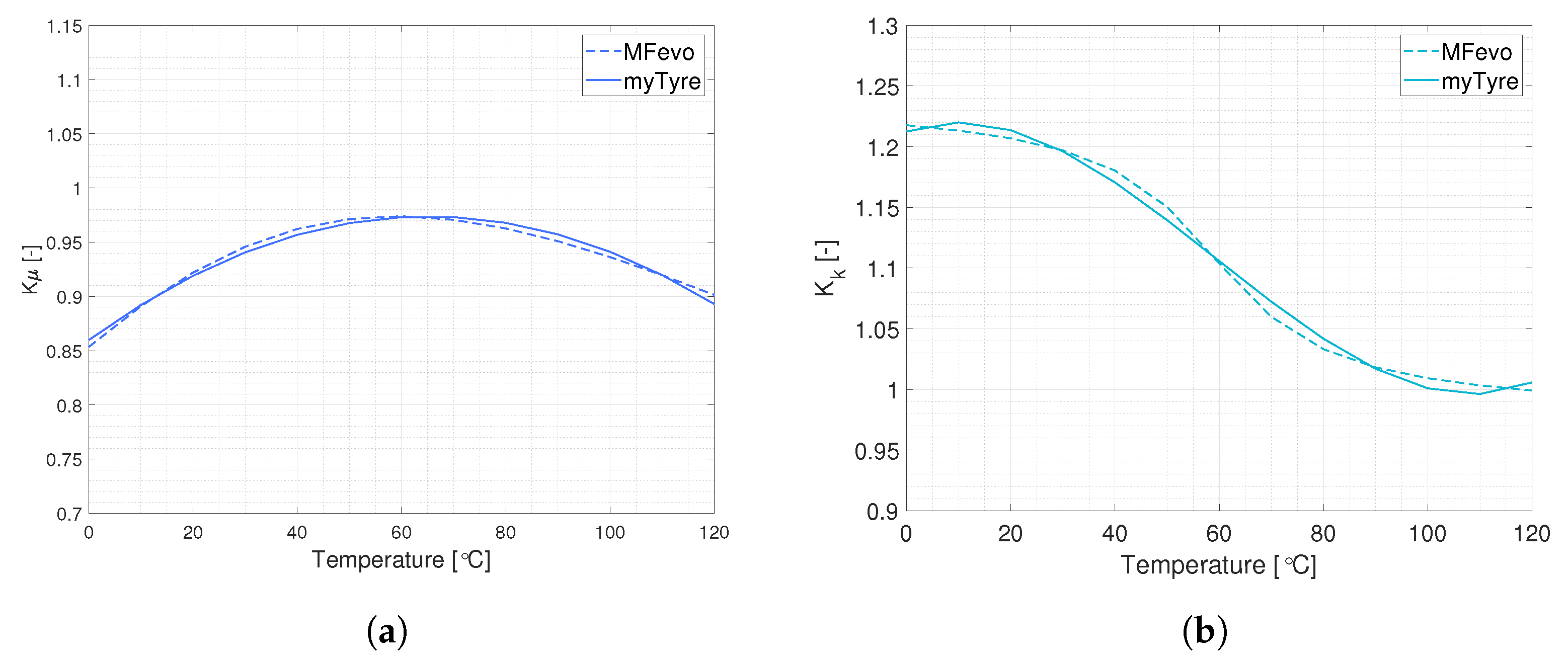
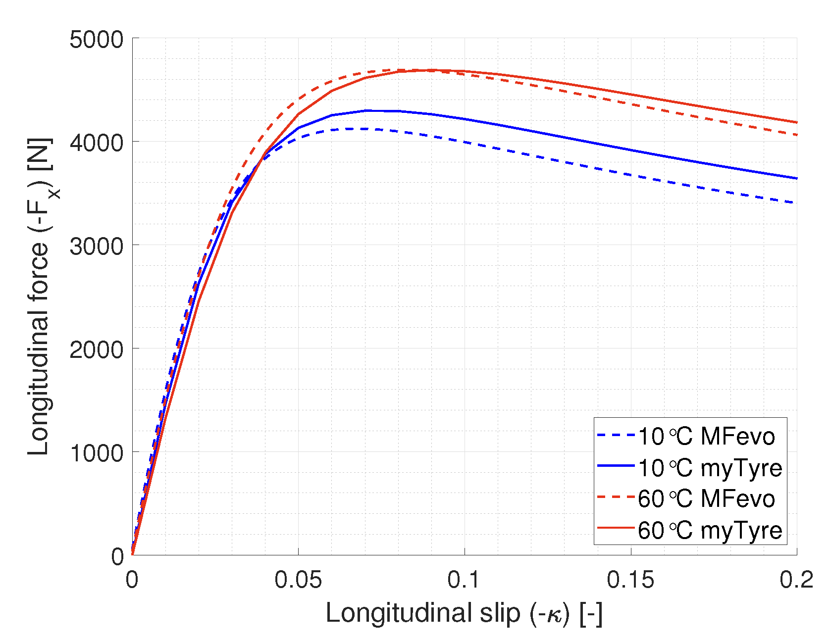
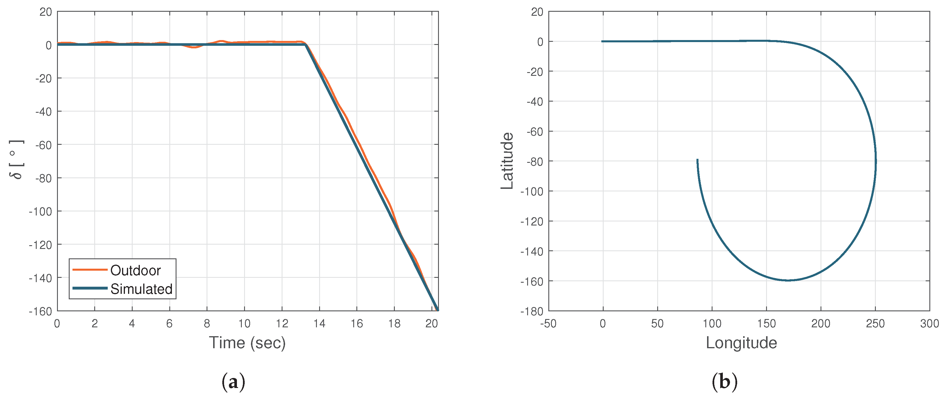
3.1. myTyre Validation

The model is made up of three sub-models, viz., Pacejka-based force equations, the thermal model, and the connecting equations.

The Pacejka force equation was fit onto the reference curve of MF-evo, which was present at the optimal temperature of 70 °C. First, the coefficients of the $C_{f\alpha }$ and $D_x$ relation were identified using separate tests for each. Based on the data, both were made linear functions of $F_z$. The three load values were chosen based on the average static load on each tyre of the reference vehicle and the maximum possible static load transfer based on the tyre peak coefficient of friction. Once, they were identified, $C_x$ and $E_x$ remained, which were identified using a non-linear numerical fitting routine. The validation plots are shown in Figure 7. For an ABS application, it is expected for the slip to not reach values much higher than the maximum force slip, so the fitting routine was kept between slip values of $[-0.15,0]$, although it is evident from the figure that the fitting will also be good until a locked wheel slip value of $-1$. The fitting was not expected to be perfect because the horizontal and vertical shift is not included in the Pacejka equation formulation used in this work. Additionally, including the vertical and horizontal shifts, and making $E_x$ a function of load, can improve the fit. However, such a fit did not pose any problems related to stability because of plant–model mismatch.

The next step was the parametrisation of the thermal model, which was performed based on the data produced from the test on full plant coupled with the MF-evo tyre. The parameters for this model are divided into two categories, viz., fixed and optimised. The fixed parameters were taken from the MFevo model. The specific heat capacity $c_t$ is taken as a constant in myTyre, and so a value around the optimal temperature was used (Figure 8). The heat transfer coefficient $h_t$ was also taken to be a constant value. The power function for the patch’s total length $l_p$ was fit onto the available data for MF-evo, as shown in Figure 8. All the final parameters are presented in

Table 1. Thermal model fixed coefficients.

Coefficient Description	Symbol	Value	Unit
Tread mass	$m_t$	2.54	kg
Tread specific heat capacity	$c_t$	1.6 × 103	$\frac{J}{Kkg}$
Tread-road heat transfer coefficient	$h_t$	4.5 × 102	$\frac{W}{m^{2}K}$
Contact patch width	$l_w$	2.9 × 10−1	m
Contact patch length function coefficient	$a_{cp}$	2.9 × 10−3	m
Contact patch length function power	$a_{cpp}$	4.9 × 10−1	−
Fraction of contact patch in sliding at zero slip	$c_{s1}$	3 × 10−1	−
Fraction of contact patch in sliding at $F_{max}$ slip	$c_{s2}$	8 × 10−1	−
$F_{max}$ slip value (assumed fixed)	${\kappa }_{max}$	1 × 10−1	−

.

For the optimised parameter fitting routines, the various input variables ($F_x$, $F_z$, $\kappa$, $V_x$, $T_t$, $T_a$) were also taken from the test, whereas in the final compiled myTyre model, the $F_x$ is fed from the simple Pacejka-based force model, as shown in Figure 2. The parameters were identified using a non-linear least squares fitting routine for a brake test of the plant with the MFevo tyre, which involved changing tyre load $F_z$ (due to load transfer), decreasing longitudinal velocity $V_x$, and changing longitudinal slip $\kappa$. The test input and output values of a front tyre were chosen and used for both front and rear tyres.

The initial and boundary conditions for this test are stated in

Table 2. myTyre thermal model validation test conditions.

Initial Conditions	Boundary Conditions
$V_{x0}$ = 40 m/s	$T_a$ = 28 °C
$T_{s0}$ = 28 °C	$T_t$ = 35 °C

.

It can be observed that the parameterisation for a given test (initial velocity and temperature, and boundary conditions) was able to reproduce the thermal behaviour for similar conditions with good accuracy, but failed to show good accuracy as these conditions changed [28]. However, because the final selected value of the prediction horizon of the full-car NMPC controller is small enough, the accuracy is always good for each prediction and the feedback of state helps update it each sampling. Hence, this same optimised parameter set was used for various tests with different initial and boundary conditions. Figure 9 shows the validation plot for the myTyre thermal model with the MFevo’s thermal test data.

Finally, the last part of myTyre, the connection between the Pacejka-based force model and the thermal model, is parameterised. The MFevo tyre model modifies the tyre peak grip and stiffness based on complicated functions of the temperature of the tread’s surface, the core, and the base layer. However, in the case of myTyre due to the availability of only the tread surface temperature, both $K_{\mu }$ and $K_k$ are a function of that (10). Multiple tests with different initial homogeneous tyre temperature were run to retrieve the values of $K_{\mu }$ and $K_k$. Final validation plots of the polynomial fitting of the functions are shown in Figure 10. The starting tyre pressure across the whole work was taken as equal to 1.4 bar, and the impact due to its changing value was not taken into account because the pressure change was extremely small in a braking manoeuvre. In the real implementation, lookup tables can be set up to compensate for the impacts of different inflation pressures on the grip and stiffness.

Figure 11 shows the performances of myTyre and MFevo for two temperature values. The thermal model was suppressed to check the performance of the Pacejka equation combined with the connecting equation (Equation (10)). The next section (Section 3.2) also shows the performance of myTyre in terms of inputs to the output longitudinal tyre force $F_x$ as compared to the MFevo and also the pure Pacejka-based tyre model (at reference temperature of 70 °C) without temperature effects.

3.2. myVeh Validation

Once the myTyre was validated, the full-car prediction model ’myVeh’ (Section 2.3.3) was finally validated. The performance of the model is shown in Figure 12. In this model, all the tyres are the same model, and hence are represented by the same parameterisation. However, in the case of real implementation, the rear tyres must definitely have different thermal model parameterisation as compared to the front because of the difference in air flow (being the biggest factor). The one-node tread model presented in this work has limited capabilities, and needs a change in the optimised parameter set to accommodate for different air flows for front and rear tyres. Nevertheless, it was assumed that the front and rear tyres of the vehicle have same airflow around them.

In this test, the same brake torque input was given to both the plant and the prediction model, and outputs were validated. All the outputs show a good fit. The tyre normal load especially had a good fit when made a state in the system, as shown in Section 2.3.3. In the transient phase of the tyre normal load, the prediction model did not fit well because of the lack of suspension modelling within, as compared to the plant model. Due to this transient phase, the longitudinal slip and force transients also suffer. The tyre longitudinal force shows a good fit overall; it is the important output, as it directly propagates how much brake torque the controller will apply, which means that mistake could lead to under or over-braking. It is clear that the velocity propagation matches perfectly, as is also important in a braking manoeuvre.

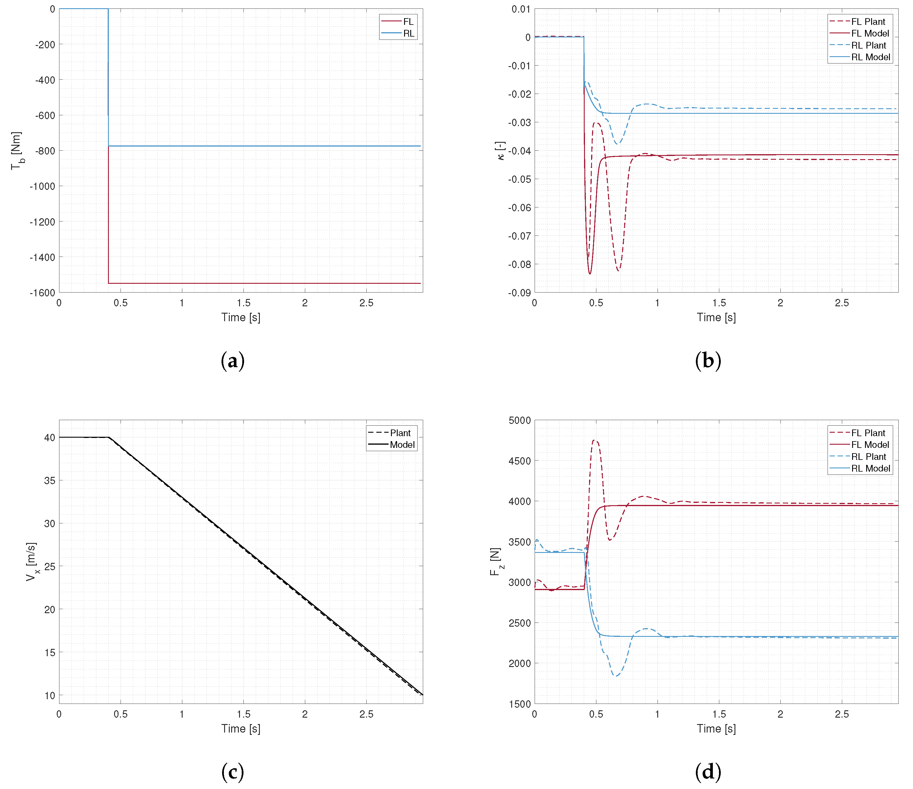
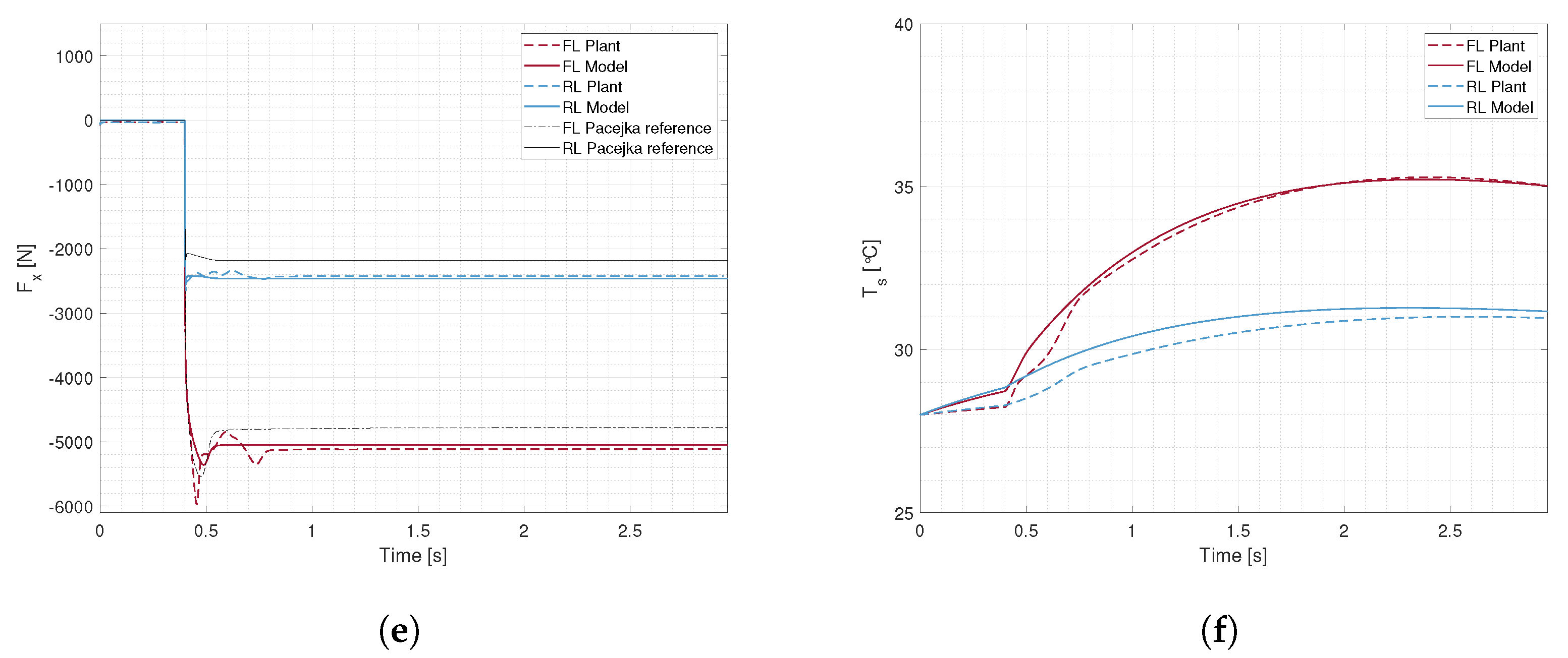
3.3. Plant Validation

In order to reproduce real car behaviour with high fidelity, the gap between simulations and experimental data has to be reduced. By exploiting a multiphysical tyre model, which consists of an evolved version of the standard MF model (MF-evo), and a vehicle model properly validated throughout experimental data acquired in outdoor testing sessions carried out with an industrial partner, it is possible to have a correct parametrisation that is able to take into account the tyre thermodynamics and wear conditions, which clearly affect tyre and vehicle dynamics [29]. The experimental data were acquired by equipping the reference vehicle with the following instrumentation:

• S-Motion: for longitudinal and lateral velocity and sideslip angle measurement.
• IMU: provides measurement of pitch, roll, and yaw rate using three rate gyros, and x, y, z acceleration.
• encoders: to detect the four wheels’ angular speeds.
• An infrared sensor for measuring the tread surface temperature.
• Internal powered pressure and IR temperature array sensor with transmitter fitted to a wheel rim, sending pressure and temperature data samples.

To increase the amount of information and to estimate the data useful for identifying the parameters of tyre interaction models used in simulations, the velocities and accelerations signal were used as input for TRICK [30]. The output provided was a sort of ’virtual telemetry’, constituting further channels with wheel slip ratio, slip angle, and tyre interaction forces. This information was used in the calibration procedure designed to parametrise the multiphysical MF-evo model. The calibration procedure consisted of three fundamental steps: the first step concerned the pre-processing of the experimental data to assess the goodness and completeness of the available dataset; the second step aimed at the identification of the standard Pacejka MF micro-coefficients in a specific thermodynamic-wear-limited range; the third one aimed at the calibration of the additional multi-physical analytical formulations, taking into account the entirety of the pre-processed dataset to extend the tyre model accuracy in the entire operating range of the tyre, comprehending thermal and degradation phenomena.

The results of the calibration process are shown in Figure 13, in which grip and stiffness dependencies towards temperature and pressure are represented. The figures are representative of the classic bell-shaped curves typical of friction coefficient variation, and the decrease in stiffness coefficient as temperature and pressure increase. These curves are valid only at a specific wear level, since the amount of grip available decreases as tread thickness decreases, whereas stiffness tends to increase as the abrasive degradation increases. To take into account that this variation, another variable dimension was added to shift these surfaces according to different wear levels.

Once properly calibrated and validated by the experimental data, this multiphysical co-simulation tyre system was employed within offline vehicle setup optimisation routines. To parameterise the vehicle model in detail, the reproduction within the simulation environment of a series of manoeuvres carried out in track testing with the real vehicle was needed. In Figure 14, the outputs of the simulations reproducing the manoeuvres performed on the track are shown: As can be noticed in Figure 15a, the manoeuvres’ inputs in terms of ramp steer and time taken to perform the test were faithfully reproduced, and this was key to good fitting based on the track data–offline simulation data comparison.

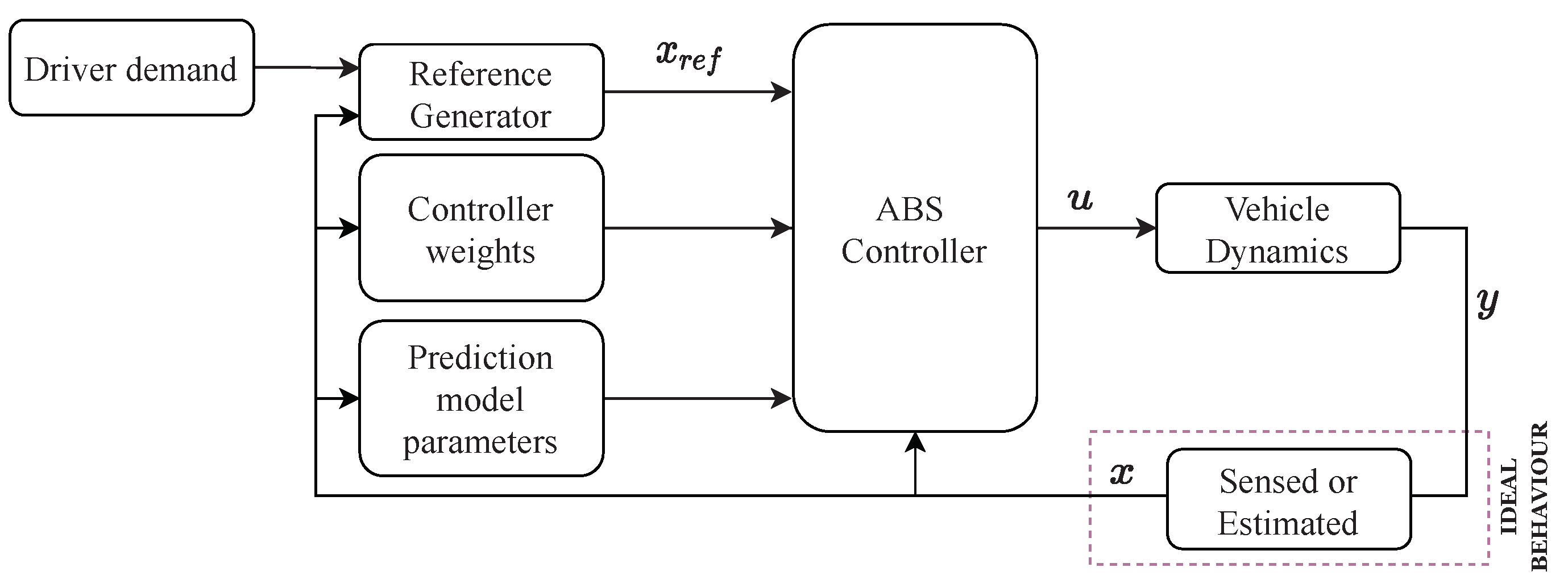
4. Controller and Simulation

All the simulations were performed in Simulink. A general data flow of the controller with the plant is shown in Figure 16. In the controller simulations, it was assumed that the ideal full-state information is available, which could be either by the means of measurement or an estimator. The whole simulation works on the assumption that everything is deterministic. The driver brake demand affects the reference for the controller, whereas the controller weights can be made dependent on the state values. The controller’s prediction model parameters can also be updated based on the different boundary conditions, as this model is not complex enough to represent the whole set of thermodynamics boundary conditions.

4.1. Quarter-Car Simulation

The quarter-car simulations were performed to get an initial understanding of the responses of the controllers, eventually helping to mitigate complex problems in the full-car simulations. The plant and prediction models in this case were kept the same, such that pure plant–model match was achieved. This helped make sure the plant–mismatch instabilities were avoided and controller performance could be assessed. The model equations used were the ones shown in Equation (16). These equations were treated differently based on the controller type—SDRE or NMPC. The next section goes into the details of the quarter-car model used in these simulations.

In these simulations, the reference and controller weighting for the controller was kept constant and not variable based on the state (as was done in the full-car simulations), to keep the analysis simple. Additionally, it is evident from the system equations that the $\kappa$ dynamics became fast as the vehicle’s longitudinal velocity $V_x$ moved towards zero. This shows that it will become difficult for the controller to stabilise the slip as the velocity decreases, as is also evident from the literature [5,31]. Hence, a cut-off velocity ($V_{x,\mathrm{cut}-\mathrm{off}}$) was set to mitigate that.

As the plant and prediction model were the same here, the description below fits both models. Based on the model in Equation (16), the state vector in this case was ${[\kappa ,V_x,T_s]}^T$, whereas the input was simply the brake torque $T_b$. The quarter-car was clearly a single-input multi-output SIMO system when the weightage on both the longitudinal slip $\kappa$ and the tread surface temperature $T_s$ were non-zero, and it was expected that kappa, being the first direct state (from $T_b$, i.e., the only input) affecting the tread temp, would be used to quickly heat the tyre in case heating was required, as was also evident in the quarter-car simulations. A lower bound ($\kappa <0$ in braking) on $\kappa$ was important to ensure that the tyre lateral force producing capability did not deteriorate too much because of running a higher longitudinal slip $\kappa$ than what was required to extract the maximum longitudinal force, and vice versa for the upper bound when the tyre was hotter than reference temperature (optimal, 70 °C, as can be seen in Figure 10a). A lower bound on the brake torque was also set to ensure a realistic brake torque saturation. A $T_b$ value a bit higher than the torque was required to lock the tyre (−2000 Nm).

The plant dynamics were simulated with a time step of 1 × 10 ^{− 3} s to capture the non-linearities of the longitudinal slip $\kappa$ dynamics which fluctuated the fastest.

4.2. Quarter-Car SDRE Controller

This section explains how the SDRE controller equations were set up, including that of the prediction model. As mentioned before, there is a need to represent the non-linear system in a linear-like SDC form. The chosen SDC representation was then checked for stabilisability across all possible sets where states and inputs can propagate.

In the SDRE, the Pacejka-based tyre force equations are left out from the controller parameterisation and the tyre force is computed externally to the SDC computation. This technique was taken from [32,33]. It helps to leave the complicated Pacejka-based tyre force function out of the SDC parameterisation, and at the same time helps with including the state dependencies within the tyre force equation.

The MARE solution was implemented, as shown in [34], which is based on the technique showed in [35]. The solution is based on the eigen-decomposition of the associated Hamiltonian matrix, as stated in [36].

4.2.1. Reference Generation

An important aspect in controllers is the definition of the reference. Here, the input for the plant is the product of the computed gain matrix and the error between the current state and the reference state:

$$u=-Ke$$

(21)

where

$$e=x-x_{ref}$$

(22)

As seen before, the reference values in the case of quarter-car are kept constant. An obvious choice for the longitudinal velocity reference is 0, as it is a braking manoeuvre. However, in the case of SDRE, it was seen that the gain computation was failing in such a case and so the reference velocity was set as follows by assuming a fixed deceleration $a_{fixed}$ of the vehicle and the reference velocity as the result of achievable velocity change within the controller sampling time step $\mathsf{\Delta }t$:

$$V_{x,ref}=V_x-a_{fixed}\mathsf{\Delta }t$$

(23)

The reference for the longitudinal slip must be kept at the value where the maximum longitudinal force is achieved. For the given parameterisation, it is seen that $-0.08$ is good compromise across different temperature values and the given mass (tyre normal force, $F_z$) of the quarter-car ($3132N$ here as the nominal tyre load of full-car). However, the reference for the longitudinal slip $\kappa$ was kept equal to $-0.1$ as a fixed value. Due to the inevitable steady state error, $-0.1$ helped with achieving the steady state slip value of around $-0.08$. Finally, the reference value for the $T_s$ was kept equal to the optimal temperature of the tyre, i.e., 70 °C for the tyre parameterisation used. However, it was seen that when the state error for $T_s$ was very high, the controller did not perform well, so based on the initial condition of $T_s$ a small initial error (by setting a lower $T_{s,ref}$ as compared to 70 °C) resulted in a better performance. For example, in the case of an initial temperature of 30 °C, a $T_{s,ref}$ = 50 °C performed much better.

4.2.2. Tuning

The controller sampling frequency was checked, and the value of 1000 Hz was important to keep the system stable; otherwise, the control of slip was very noisy (smaller controller frequencies). Even with a value of 1000 Hz, the controller oscillated to some extent when the vehicle velocity was lower than 14 m/s, but because of the cut-off velocity of 10 m/s, this was not a problem. There was no possibility of tuning the prediction horizon, as it was set to infinity in the SDRE setup.

The tuning of weights in an optimal-control-based controller is much simpler than in a conventional controller because the weights are directly connected to the state variables. For the start of tuning, the technique of setting the corresponding state weighting as a reciprocal of the square of its maximum achievable value $q_{ii}=1/x_{i,max}^2$ [37] did not help in terms of achieving a solution for gain computation, but it gave an idea about where to start. Additionally, Mehmet et al. [38] showed that tuning of an SDRE controller is not a straightforward procedure and requires some trial and error. Eventually, it was seen that the final weighting for $\kappa$ needed to be very large because of the fast dynamics. The weighting on the $V_x$ did not show any performance benefit, and the weighting on $T_s$ was non-zero only in the case where optimising the tyre temperature was important. Any weighting on the control input $T_b$ would result in suppressing the optimally calculated torque, so it was kept equal to 0. All final weightings are stated in

Table 3. Quarter-car (QC) controller weights.

		QC-SDRE		QC-NMPC
State	Weight Variable	Value: κ-Control	Value: κ and ${\mathit{T}}_{\mathbf{s}}$-Control	Value: κ-Control	Value: κ and ${\mathit{T}}_{\mathbf{s}}$-Control
κ	$q_{\kappa }$	1 × 1010	1 × 1010	1 × 104	1 × 104
$V_x$	$q_{V_x}$	1 × 10−1	1 × 10−1	0	0
$T_s$	$q_{T_s}$	0	1 ×106	0	5

. The first case is the pure control of $\kappa$ only (while a feasible numerical solution of the gain is achieved with a non-zero weighting on $V_x$), and another case is where weighting is also given to control $T_s$, which helps with optimising the tyre temperature that may achieve higher grip overall but at least heat the tyre faster, which can help to simply heat the tyre quicker over multiple braking manoeuvres.

4.3. Quarter-Car NMPC Controller

This sections explains how the NMPC controller equations were set up, including that of the prediction model. Here, the prediction model is presented in the non-linear state-space format, as shown in Equation (16) in an implicit form. Here, the full non-linear model, including the non-linear tyre equation, was computed within the controller and not externally, as seen in SDRE.

In NMPC it is also possible to set state and input bounds within the optimisation computation. In this work, mainly the bounds on $\kappa$ and $T_b$ are important and were implemented (as discussed in Section 4.1). The MATMPC toolbox requires multiple settings relevant to the numerical solution which are defined in

Table 4. NMPC—MATMPC toolbox settings used.

Setting Parameter	Value
Hessian approximation	Gauss–Newton
Integrator-type	Implicit Runge–Kutta 3rd order
QP condensing	full
QP solver	qpOASES (full-condensed QP)
hotstart	no
RTI scheme	no

.

In this work, for the objective function (24):

$$\begin{array}{cc}\hfill & \genfrac{}{}{0pt}{}{minimise}{\mathbf{y}\left(·\right),\mathbf{u}\left(·\right)}{\int }_{t_0}^{t_0+T_P}\left({∥y\left(t\right)-y_{ref}\left(t\right)∥}_Q^2+{∥u\left(t\right)-u_{ref}\left(t\right)∥}_R^2\right)dt\hfill \\ \hfill & +{∥y(t_0+T_P)-y_{ref}(t_0+T_P)∥}_P^2\hfill \end{array}$$

(24)

The output vector $y\left(t\right)$ and the the terminal output vector $y(t_0+T_P)$ are the same as the state vector ${[\kappa .V_x,T_s]}^T$.

4.3.1. Reference Generation

The reference for $\kappa$ was kept the same as in the quarter-car SDRE, as shown in Section 4.2.1. For $V_x$ the reference was simply kept equal to 0 because it is a braking manoeuvre and the car aimed to stop/slow down. Additionally, the reference for $T_s$ was kept equal to the optimal temperature value 70 °C for the tyre, as it was easy to achieve consistent performance across different conditions in the NMPC controller, and a changing $T_{s,ref}$ was not needed, as in SDRE. A non-uniform grid of references is also possible in the NMPC-based controller but currently is not available within the MATMPC toolbox. Although the performance without that is satisfactory, it will only increase the number of tuning variables, thereby complicating the development.

4.3.2. Tuning

For the controller sampling time $T_s$, the fastest and unstable dynamics of the system are important to consider (here $\dot{\kappa }$). The $\kappa$ dynamics are seen to be around 20–30 Hz, as is also seen in the literature. As a rule of thumb in control theory, the controller’s sampling time must be 4–10 times faster than that of the process time constant. The faster the controller, the easier it will be to catch the changes in the states of the system, such that they can be controlled. Considering the 20 Hz of $\dot{\kappa }$, we see that at least 100 Hz (five times) of controller frequency is necessary. Based on that, three values for the controller frequency were chosen [100, 150, 200] Hz, corresponding to [10,7,5] ms of sampling time $T_s$. The difference between the rise time for a step change in $\kappa$ is seen to be within 5 ms, and so the smallest value of 100 Hz was chosen. In terms of settling time, it lags only by 10 ms and has a negligible overshoot. For these tests, only the slip state was weighted (with a value of $1\times {10}^4$) and the number of horizon steps (N) was kept constant at two, corresponding to prediction horizons of [20,14,10] ms.

Now comes the selection of the prediction horizon ($T_P$ with N samples). Increasing N is costlier in terms of computation; on the other hand, it helps the controller look into the future and improve stability. In this work, increasing N also helps in controlling $T_s$ (by running a higher $\left|\kappa \right|$ initially to heat the tyre quickly and then come back to zero error in slip). However, the same effect is also seen by increasing the relative weight on the $T_s$. Between N and the weight on $T_s$, N is more costly, as it has a direct positive correlation with the computation time of the controller. Although the computation time is out of scope of this thesis, but in the future if this technique is implemented then computational time will become a big factor for real-time performance.

Once the controller settings ($T_s$ and N) were selected, focus was shifted towards the weights set on the state and control input in the cost function (24). As NMPC is a model-based controller, this led to the tuning being done based on the parameters directly connected with the states of the system model. Additionally, another benefit is the fact that the numbers of tuning parameters are less as compared to the industry standard rule-based controllers such as the ABS in production cars [5].

As is seen in the quarter-car system model (16), there are three states, i.e., $x=[\kappa ,V_x,T_s]$, with the control input being $u=T_b$. It is obvious not to put any non-zero weight on the control input $T_b$, as that would lead to suppressing the optimal $T_b$ value. In an ABS system, meeting the objective of generating the maximum longitudinal force (or maximum longitudinal acceleration) while maintaining steer ability is simply done by following the reference set for the optimum longitudinal slip $\kappa$. If the reference longitudinal slip $\kappa$ is maintained, it will automatically ensure that the desired velocity of 0 ($V_{des}=0$) is met as soon as possible, so the weighting on it was set to zero. Additionally, the weight on $\kappa$ was decided on by using a range of values. It is seen that a weight of $1e4$ is sufficient, and increasing the weight beyond that did not result in any reductions in rise time to a step response.

Finally, the weight on $T_s$ produced two cases, as seen in Section 4.2.2 and Table 3. For the case of only $\kappa$ control (Case 1), the weight $q_{T_s}$ was simply 0. Additionally, in the case of $\kappa$ and $T_s$ control (Case 2), the weight $q_{T_s}$ was non-zero. Although the quarter-car was not tested extensively across a range of initial and boundary conditions, by some preliminary tests it was evident that varying the $q_{T_s}$ with the initial conditions of $T_s$ and $V_x$ in a braking manoeuvre and also making it 0 when the velocity dropped below a certain threshold ($V_{x,cut-off}$ = 20 m/s here) helped with a consistent performance. It is clear that in a braking manoeuvre, as the velocity drops, the heating of the tyre stagnates; thus, heating the tyre provides no benefit after that, so the weight for $T_s$ was made 0 below this $V_{x,cut-off}$. Finally, this concept of variable weights is used in the full-car NMPC controller. Table 3 states the chosen weights in the case of quarter-car NMPC, tested on a case with $T_{s0}$ = 30 °C, $V_{x0}$ = 40 m/s and boundary conditions of $T_a$ = 28 °C, and $T_t$ = 35 °C. For the lower bound on $\kappa$, an arbitrary value of $-0.12$ was chosen. For real implementation, there can be a number of factors that can affect the choice. To name a few, drop in lateral grip, the hydraulic system’s capability to stabilise the slip beyond the peak, gains in temperature, gains in braking distance performance, etc., can affect the choice.

4.4. Full-Car Simulation and NMPC Controller

The quarter-car simulations already give a good idea on how the system will respond without representing all the details of the full-car, but to see the real world applicability, the details such as the connection between the 4-wheels and load transfer are important to consider. The full-car simulation data-flow architecture which is representative of the setup in Simulink is shown in Figure 16. The plant used in these simulations was completely different than the prediction model inside the controller. The plant was composed of the full-car model coupled with the MF-evo, whereas the prediction model was the ’myVeh’, as defined in Section 2.3.3.

For the full-car simulations we chose to move forward only with the NMPC-based controller because the implementation of the SDRE-based controller on the quarter-car showed infeasibility in MARE solutions and would have become even more complicated to debug in the case of a full-car. Additionally, the instability of the quarter-car SDRE controller was high as compared to the NMPC one (Figure 17 and Figure 18). In this respect, the NMPC showed good robustness in terms of tuning the system.

The concerned states in the full-car case were simply based on the states that were modelled in the prediction model ’myVeh’, $x={[{\kappa }_1,{\kappa }_2,{\kappa }_3,{\kappa }_4,V_x,T_{s1},T_{s2},T_{s3},T_{s4},\mathsf{\Delta }{F}_z]}^T$. These state variables were especially required, as feedback from the plant as the NMPC-based control requires full-state feedback. The subscript numbers here are defined for each wheel, as were also described in Section 2.3.3. Here, the control input was $u={[T_{b1},T_{b2},T_{b3},T_{b4}]}^T$, i.e., the brake torques corresponding to each wheel. As will be discussed below, the references were made variable based on the state feedback, and some of the weights were also made functions of initial conditions and the state feedback. The lower bound on the $\kappa$ belonging to the rear wheels was tighter as compared to the front wheels to ensure stable behaviour (${\kappa }_{1,bound}=-0.12$ and ${\kappa }_{3,bound}=-0.11$). An accurate quantification of these bounds must depend on a real application. Additionally, the torque bounds on the front and rear wheels were different (front higher than the rear—$T_{b1,bound}=-2200$ Nm and $T_{b3,bound}=-2000$ Nm), set higher than the wheel locking limits, as was also discussed in Section 4.1. Lastly, the plant dynamics were simulated with a time step of 1 × 10⁻³ s to capture the non-linearities of the system.

The representation of the prediction model was prepared in the same way as described in Section 4.3. The optimisation at each controller sampling instant was performed with the MATMPC toolbox with the settings defined in Table 4. The cases of in-feasibility were not discovered in the work, so no such techniques such as limiting the maximum iterations were applied. For the objective function (24), the output vector $y\left(t\right)$ and the terminal output vector $y(t_0+T_P)$ were the same as the state vector $x={[{\kappa }_1,{\kappa }_2,{\kappa }_3,{\kappa }_4,V_x,T_{s1},T_{s2},T_{s3},T_{s4},\mathsf{\Delta }{F}_z]}^T$, and the input vector was $u={[T_{s1},T_{s2},T_{s3},T_{s4}]}^T$.

4.4.1. Reference Generation

Here, the reference for the ${\kappa }_i$ was especially required to be variable with the state, as the peak of the $F_x$ characteristic curve moved with changing load. In addition, the impact of the tread temperature was also included. The ${\kappa }_{max}$ values as a function for the reference tyre model were as shown in Figure 19. As seen in the quarter-car NMPC controller, the reference for $V_x$ was set to 0. Additionally, for the load transfer state $\mathsf{\Delta }{F}_z$, there was no concern about controlling it, so the reference and weight were set as 0. Finally, as seen in Section 4.3.1, the reference for the tread temperatures of all the tyres was set as 70 °C.

4.4.2. Tuning

In a full-car simulation, the tyres experience changing loads, especially because of the longitudinal load transfer in braking. This leads to a change in the sharpness of the peaks of tyre characteristic curves; the tyres with higher loads have especially sharper $F_{x}vs.\kappa$ peaks. In a braking manoeuvre, the front tyres experience higher loads. Due to this reason, it becomes difficult for the controller to stabilise ${\kappa }_{1/2}$, as was seen in the preliminary tests, especially when the vehicle velocity was small. To mitigate this, it was seen that increasing the controller’s sampling frequency made a huge difference. Thus, the adequate controller sampling frequency was clearly 1000 Hz, which still struggled to stabilise the ${\kappa }_{1/2}$ at the steady-state value with a zero error. The prediction horizon $T_P$ was kept the same as 20 ms, which led to $N=20$, as seen in the case of quarter-car NMPC Section 4.3.2.

Coming to the weights in the cost function (24), first, the weights for the ${\kappa }_i$ ($q_{{\kappa }_i}$) were finalised; a higher weight was given to the slip of the front wheels to ensure stability because of the reason of higher load, as explained above. The weights related to $V_x$ and $\mathsf{\Delta }{F}_z$ ($q_{V_x}$ and $q_{\mathsf{\Delta }{F}_z}$) were kept equal to 0, as is explained in the reference generation section above.

As seen in Section 4.3.2, the weights related to the tread temperature for the case of ($\kappa$ and $T_s$)-control were made a function of the initial conditions $T_{s0}$ and $V_{x0}$, including the zero value when $V_x$ < 20 m/s (as shown for $q_{T_s}$ in Table 3). Of course, the values for the weights on $T_{si}$ in the full-car case were different, but the dependencies were similar to the quarter-car case. This was achieved with the use of a look-up table in Simulink, which is depicted in Figure 19. The variable weights for $T_{si}$ ($q_{T_{si}}$) were chosen based on tests with different initial conditions, and to achieve a consistent overall performance, the weight values were tuned. Specifically, as the ($q_{T_{si}}$) values were non-zero only in the case of ($\kappa$ and $T_s$)-control, it was made sure that the increase in braking distance did not rise higher than $2\%$, and the maximum temperature in the manoeuvre was at least greater than $5\%$ as compared to the pure $\kappa$-control case. The final weights used were those shown in

Table 5. Full-car NMPC controller weights.

State	Weight Variable	Value: $\mathit{\kappa }$-Control	Value: $\mathit{\kappa }$ and ${\mathit{T}}_{\mathit{s}}$-Control
${\kappa }_1$	$q_{{\kappa }_1}$	1 × 104	1 × 104
${\kappa }_3$	$q_{{\kappa }_3}$	1 × 103	1 × 103
$V_x$	$q_{V_x}$	0	0
$T_{s1}$	$q_{T_{s1}}$	0	$f(T_{s0},V_{x0})$ and $0\iff (V_x$<$20\vee \frac{d{T}_s}{dt}$<$0)$ (Figure 19B)
$T_{s3}$	$q_{T_{s3}}$	0	$f(T_{s0},V_{x0})$ and $0\iff (V_x$<$20\vee \frac{d{T}_s}{dt}$<$0)$ (Figure 19B)
$\mathsf{\Delta }{F}_z$	$q_{\mathsf{\Delta }{F}_z}$	0	0

. As the vehicle model is symmetric, the left ($1,3$) and right ($2,4$) values were the same, so only the values for the left are stated.

5. Tests and Metrics

There were three final full-car controller setups used for the final tests. These three setups are explained in the following:

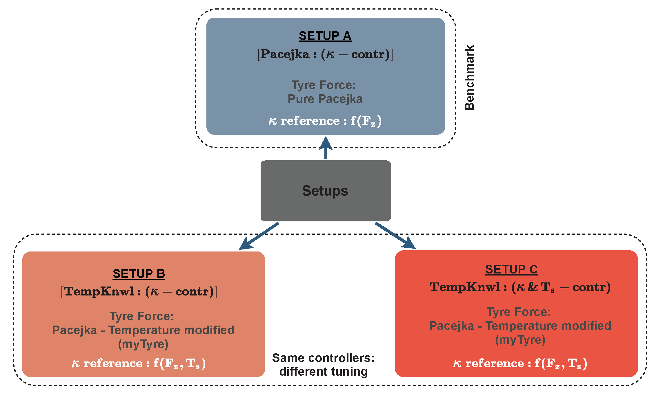
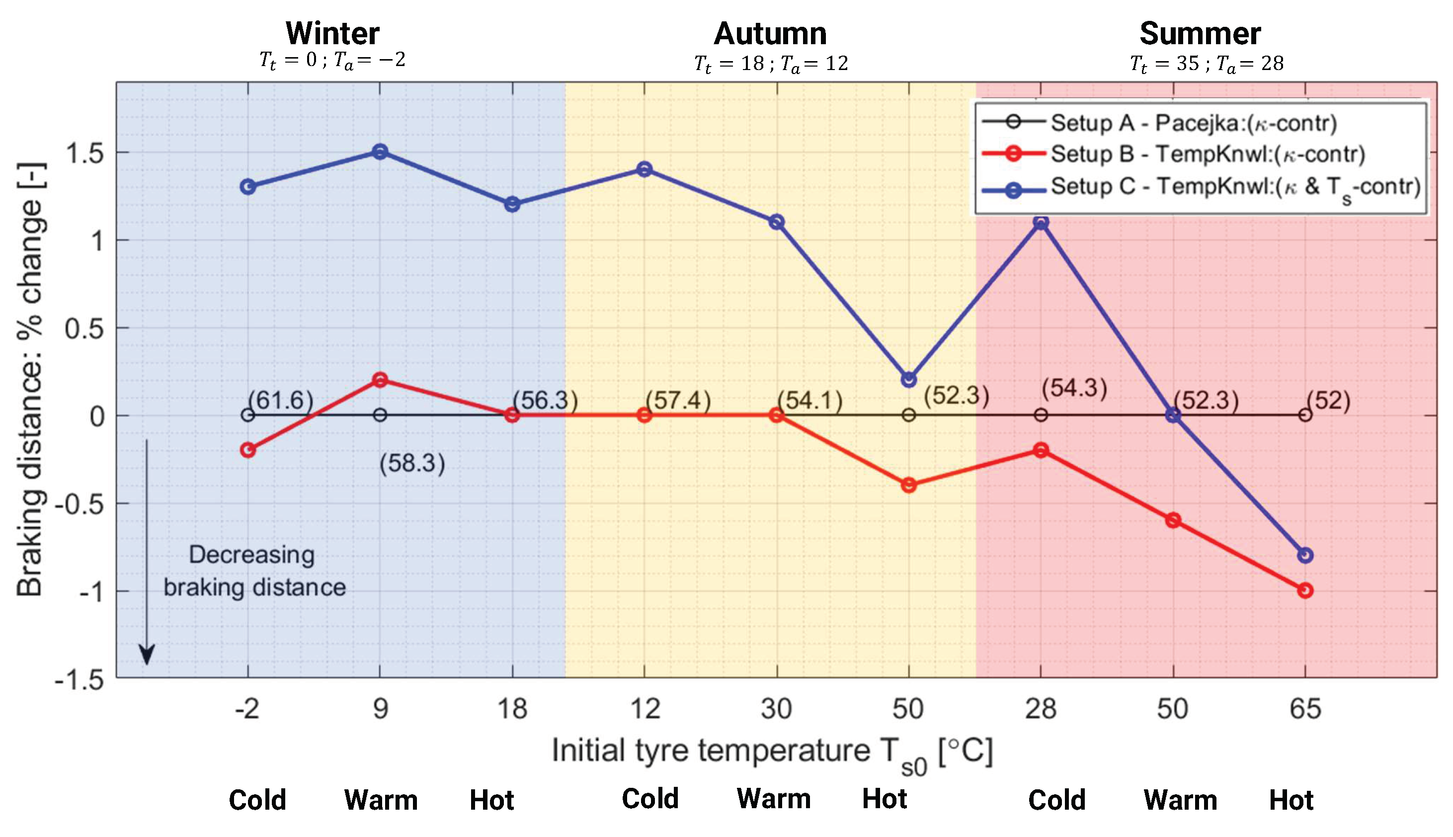
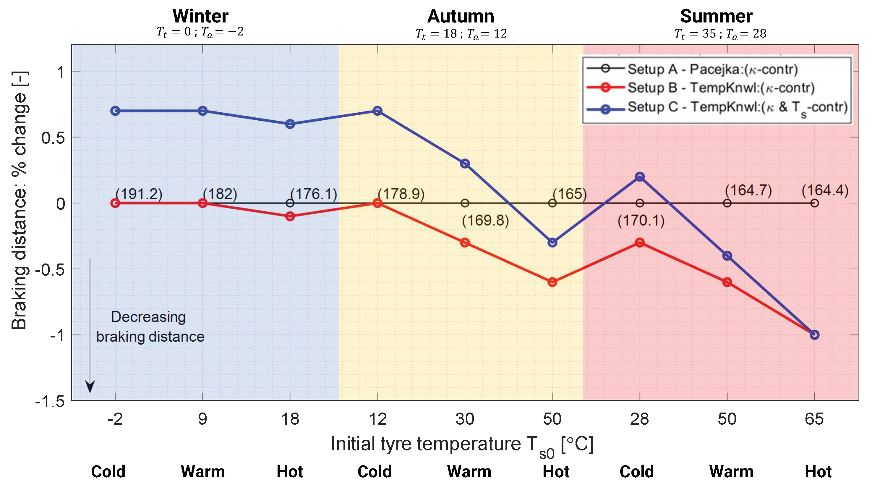
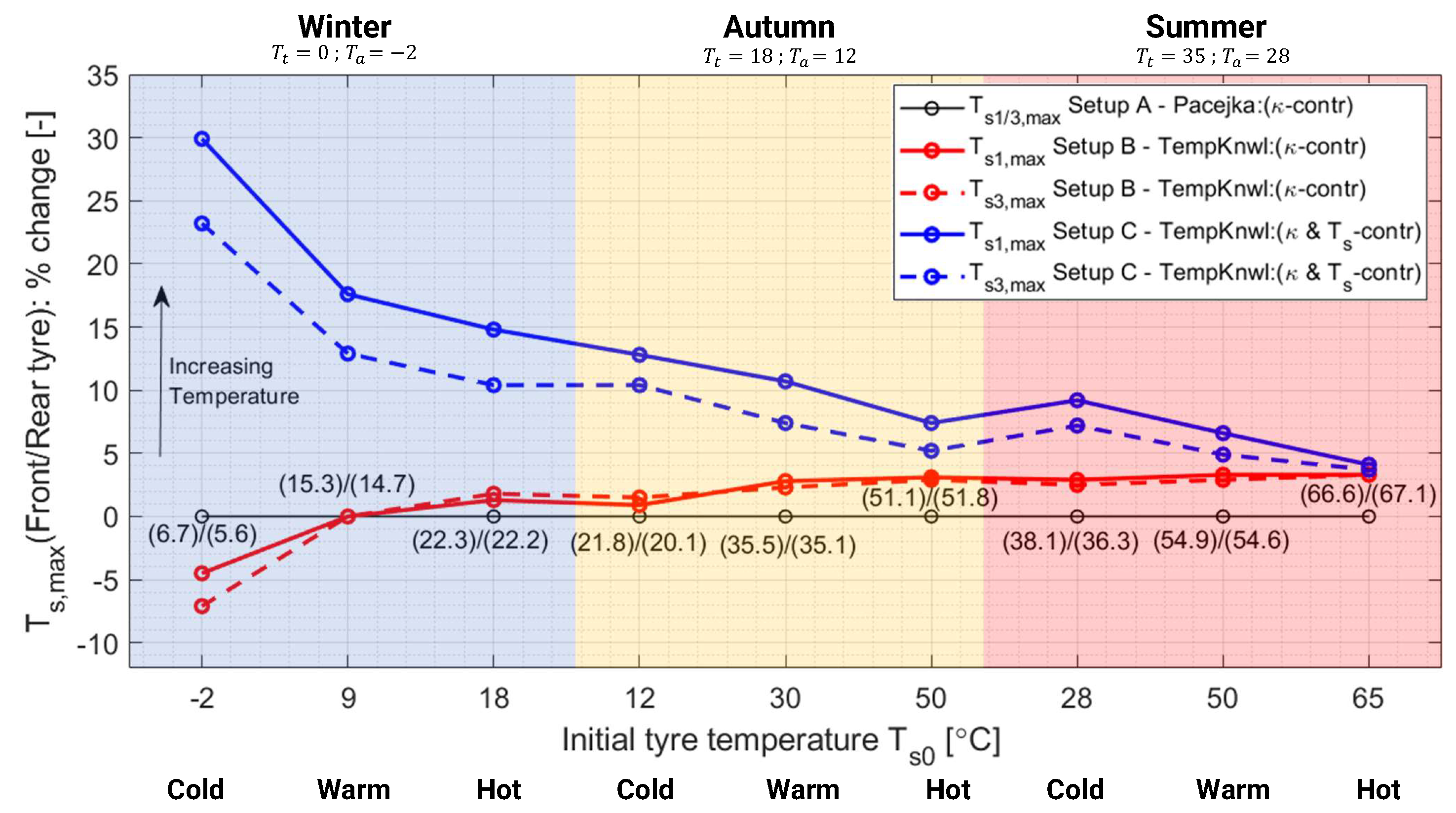
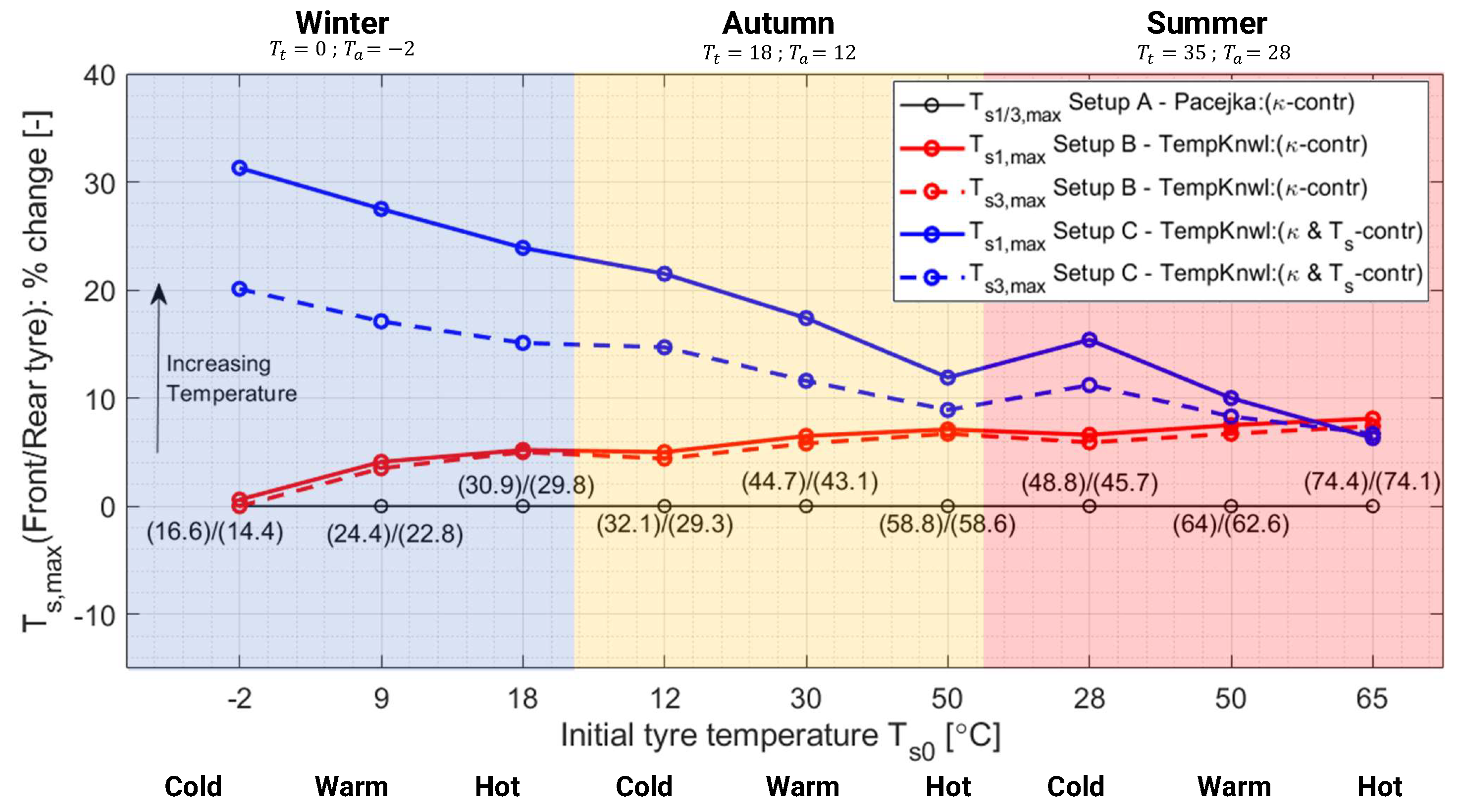
5.1. Controller Setups

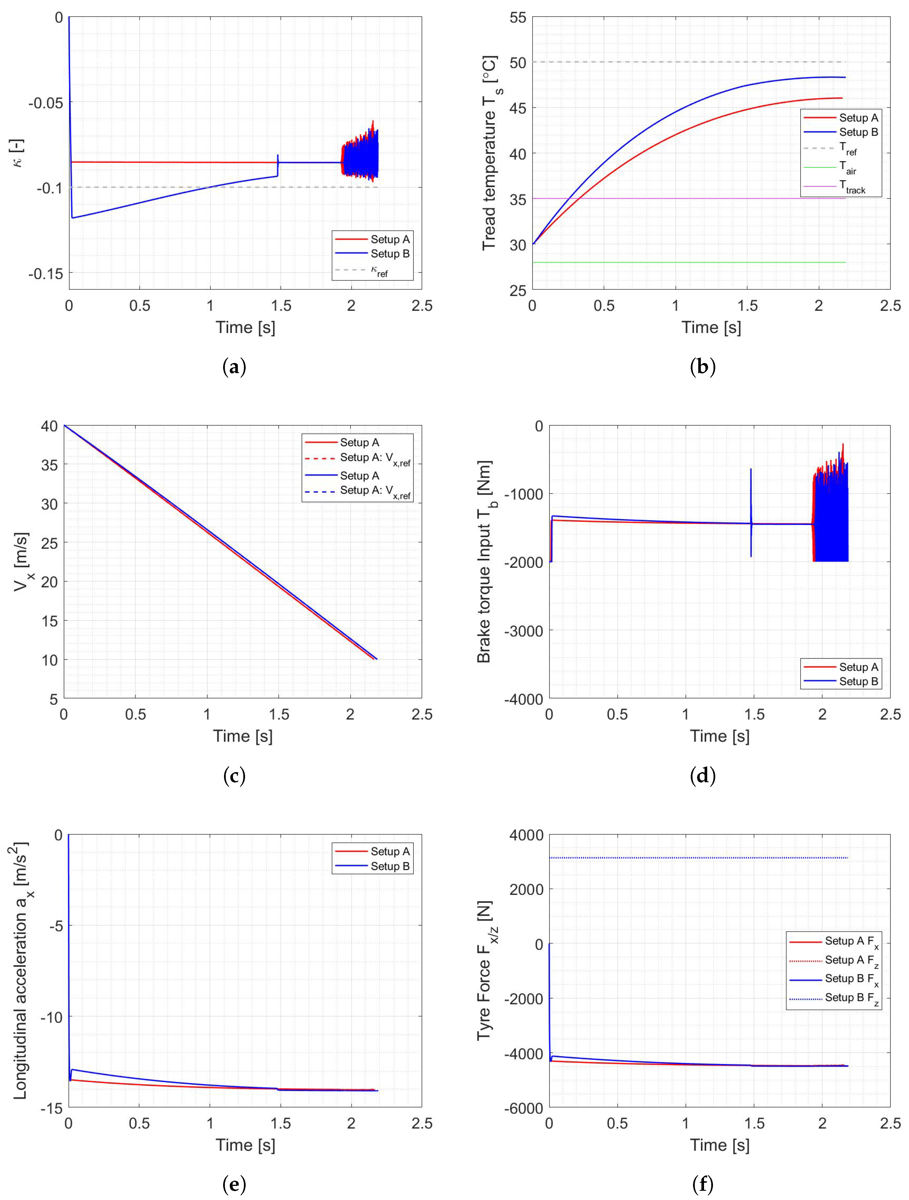
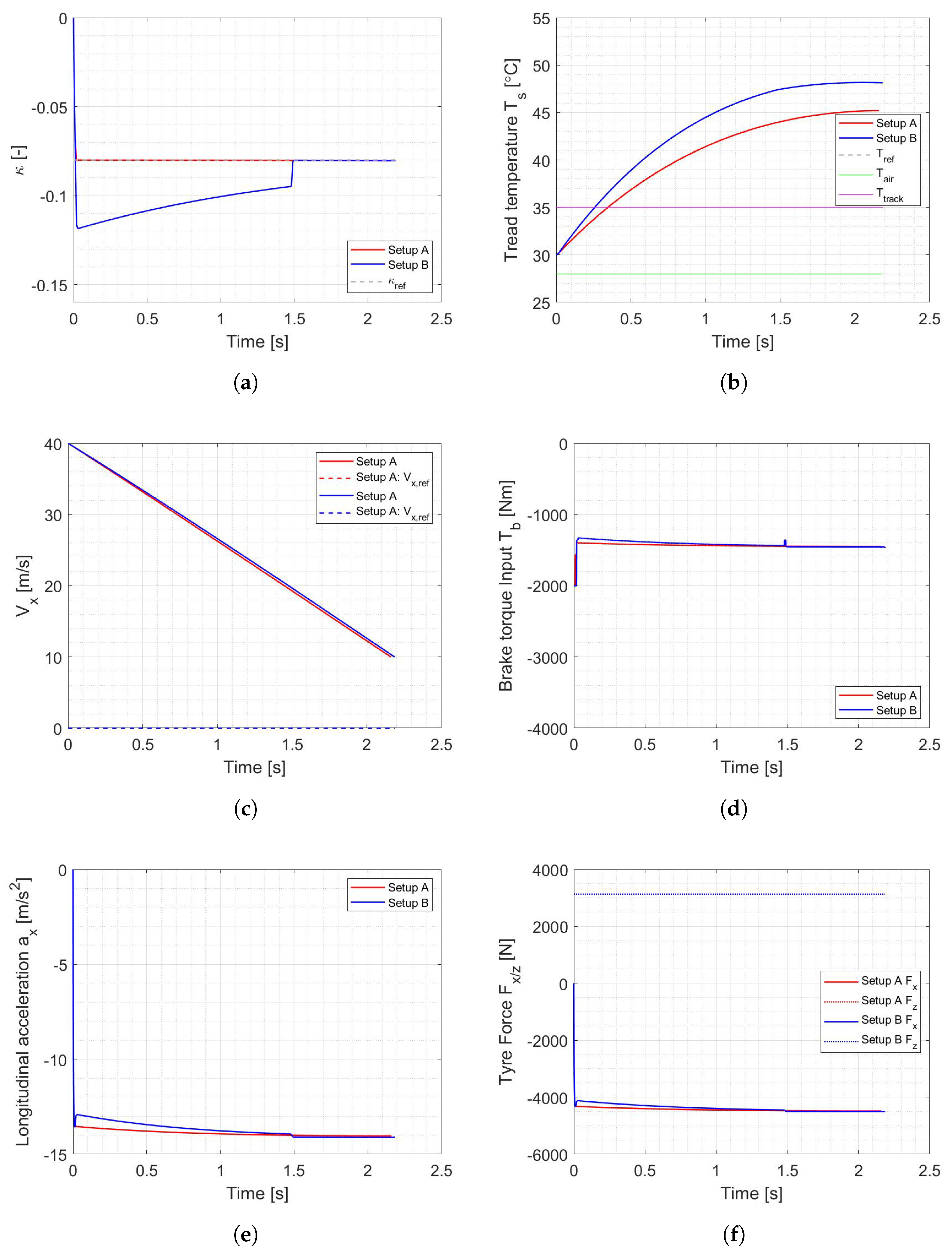
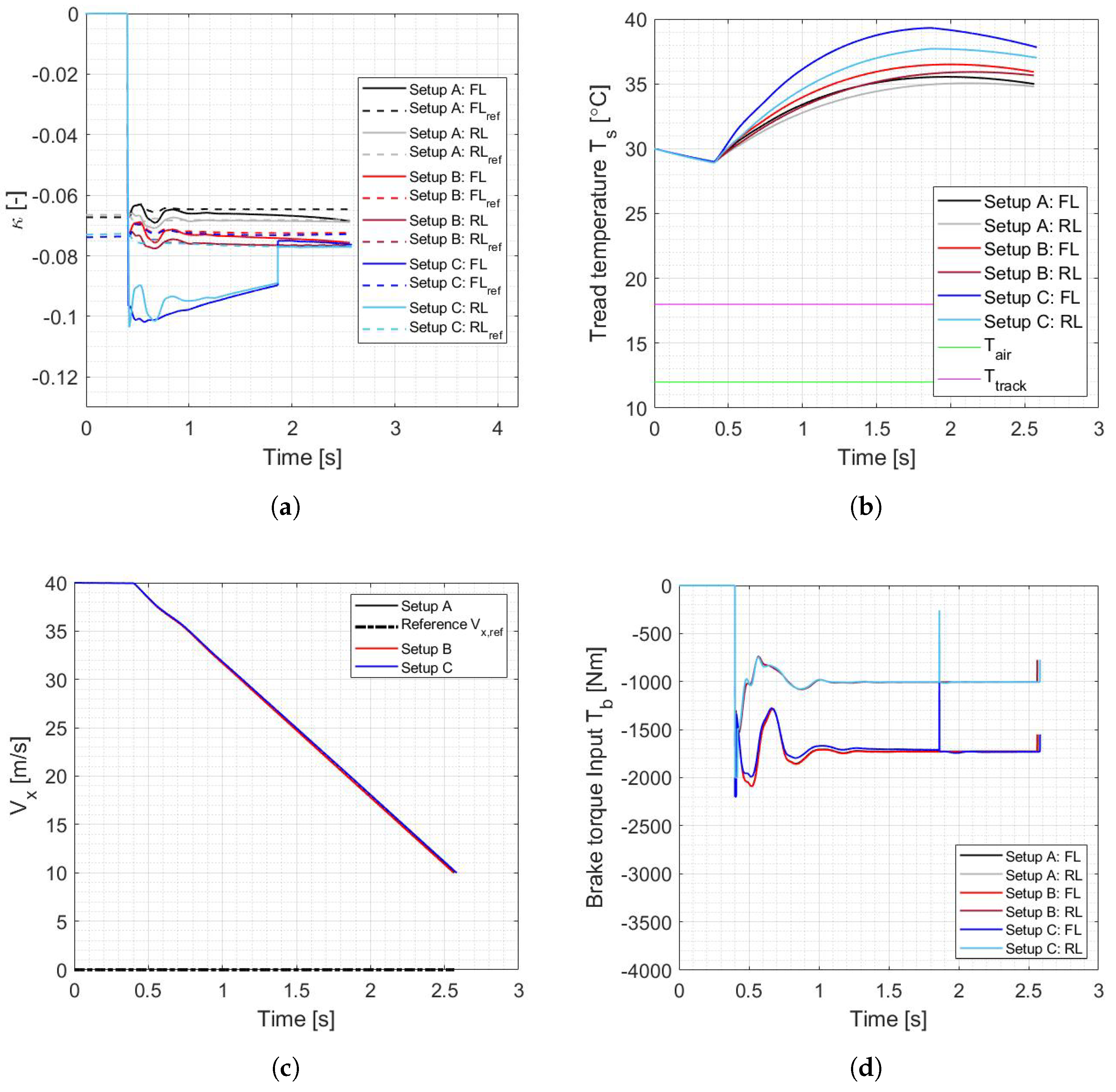
• Setup A [Pacejka:($\kappa$-contr)]: This controller setup’s prediction model consists of an ’myVeh’ model with the reference Pacejka model (as used in ’myTyre’) without any tread surface temperature dynamics (so states ${[T_{s1},T_{s2},T_{s3},T_{s4}]}^T$ are not available). Hence, the prediction model only consists of six states ${[{\kappa }_1,{\kappa }_2,{\kappa }_3,{\kappa }_4,V_x,\mathsf{\Delta }{F}_z]}^T$. The parameterisation of this tyre model is taken as that of the tyre operating at (40 °C). Such a setup, to a good extent, replicates the controller shown by Pretagostini et al. [5], which he showed performs much better than the state-of-the-art rule-based controllers. The only difference here is that the first-order torque rate dynamics are not considered inside the prediction model, and the tyre force equations are included inside the controller instead of feeding them as inputs from wheel load sensors. Hence, this setup can be considered a benchmark for this work and results of the proposed controller setups (Setup B and C) can be compared relative to this setup. As regards the selection of tyre force model’s parameterisation at 40 °C, it is like representing the tyre behaviour that acts like an average amongst the whole range of $T_{s0}$ shown in Figure 20. Even when a parameterisation at some other temperature is selected, the controller’s performance is expected to degrade at temperatures far above or below that. The reference generation being another important factor, Pretagostini et al. [5] used the slip reference input as a function of tyre load $F_z$ for the the parameterisation used in their work. In this work, the reference was taken as the value that could perform well across the whole temperature range and maintain stable behaviour (not go beyond the peak of $F_x$ characteristic). Thus, here, the reference generation was only a function of the tyre normal load ($F_z$). Such a setup of parameterisation and the reference slip values helps a controller with no knowledge of temperature to perform good enough across all the tests. The controller weights on the longitudinal slips (${\kappa }_i$) were set as shown in Section 4.4.2. For ease of readability, it is named ’Pacejka:($\kappa$-contr)’, meaning that its tyre model is only based on the Pacejka tyre force equation and has no temperature effects, and only tries to control the longitudinal slips, i.e., ${\kappa }_i$.
• Setup B [TempKnwl:($\kappa$-contr)]: This controller setup’s prediction model consists of the full ’myVeh’ (Section 2.3.3) model combined with the ’myTyre’, i.e., with the tread surface temperature dynamics. Hence, this controller is able to also predict the change in tyre grip and stiffness with the changing temperature conditions throughout and between each test. This helps it control the tyre slip more precisely as compared to Setup A Pacejka:($\kappa$-contr). Here, the controller weights are non-zero only for the longitudinal slips (${\kappa }_i$) and equal to the values used for Setup A (as defined for the case of $\kappa$-control in Table 5). For convenience, it is named ’TempKnwl:($\kappa$-contr)’, meaning that it has the temperature knowledge (TempKnwl) and just controls the ${\kappa }_i$.
• Setup C [TempKnwl:($\kappa$ & $T_s$-contr)]: This controller setup is the same as that described in Setup B, with the slight difference being that, here the controller weights on tyre tread temperature states ($T_{si}$) are non-zero (as defined for the case of $\kappa$ and $T_s$-control in Table 5). Especially, the weighting on $T_s$ is kept non-zero to check how heating the tyre more towards the optimal temperature could help in terms of braking distance. For convenience, it is named ’TempKnwl:($\kappa$ & $T_s$-contr)’, meaning that it has the same temperature knowledge as Setup B, and it tries to control the ${\kappa }_i$ and the $T_{si}$. Hence, Setup B and Setup C only differ in terms of the weights (Figure 21).

Setup B acts like a controller that has better knowledge of the plant dynamics as compared to Setup A, so these two were compared in the various tests. Additionally, Setup C was used to optimise the tyre temperature while ensuring the slip dynamics are stable, which can potentially lead to faster heating times or possible reduction in the braking distance as compared to both the other setups. Hence, for all the described tests, these three controllers are compared while keeping Setup A as the reference/benchmark.

5.2. Tests

The manoeuvre performed was a braking manoeuvre starting at some initial velocity $V_{x0}$, and then a full brake demand was provided by the driver, which activated the NMPC-based ABS, eventually leading to optimally calculated brake torques going to each wheel. The road was assumed to be smooth with a coefficient of friction of 1. As our main concern lies in thermodynamic boundary conditions, various tests with different track ($T_t$) and ambient ($T_a$) temperatures (fixed boundary conditions) were chosen, relating to three different weather conditions, viz., winter, autumn/spring, and summer. For each of these boundary conditions, three initial condition temperatures were defined in the tests, viz., cold, warm, and hot. These tests were then performed with two different initial velocities, viz., 40 and 70 m/s. Two initial velocities were chosen, as the temperature behaviour is linked to friction power, and convection is highly dependent on the velocity. In each test, the simulation was stopped at 10 m/s concerning the controller’s instability at lower velocities (as can be seen in the $\dot{\kappa }$ Equation (12) and is also discussed in Section 4.1). In total, there were 18 tests per controller setup, as shown in Figure 20. The test names (Test 1, Test 2,...) shown in this figure and the setups previously mentioned were used.

To assess the performance of each setup, there must be some metrics defined to quantify the time history of various state variables. As this work mainly focused on high-level controller decision making, it was not necessary to include all the metrics that are generally used to assess ABS performance (such as human-related factors). Additionally, as the number of tests was large due to the various boundary conditions, it was better to choose a few important factors than a variety.

Here, for each test, two main metrics were chosen to assess the performances of the proposed controller setups:

• Braking distance ($s_{br}$): This is defined as the distance the vehicle covers from the time the brake input is given to the time it reaches the set cut-off velocity ($V_{x,cut-off}$) of 10 m/s, as defined above. As the main objective of ABS is to ensure the tyre delivers the maximum possible force, braking distance is the perfect metric for that. To assess the performance of this high-level controller, this metric is sufficient.
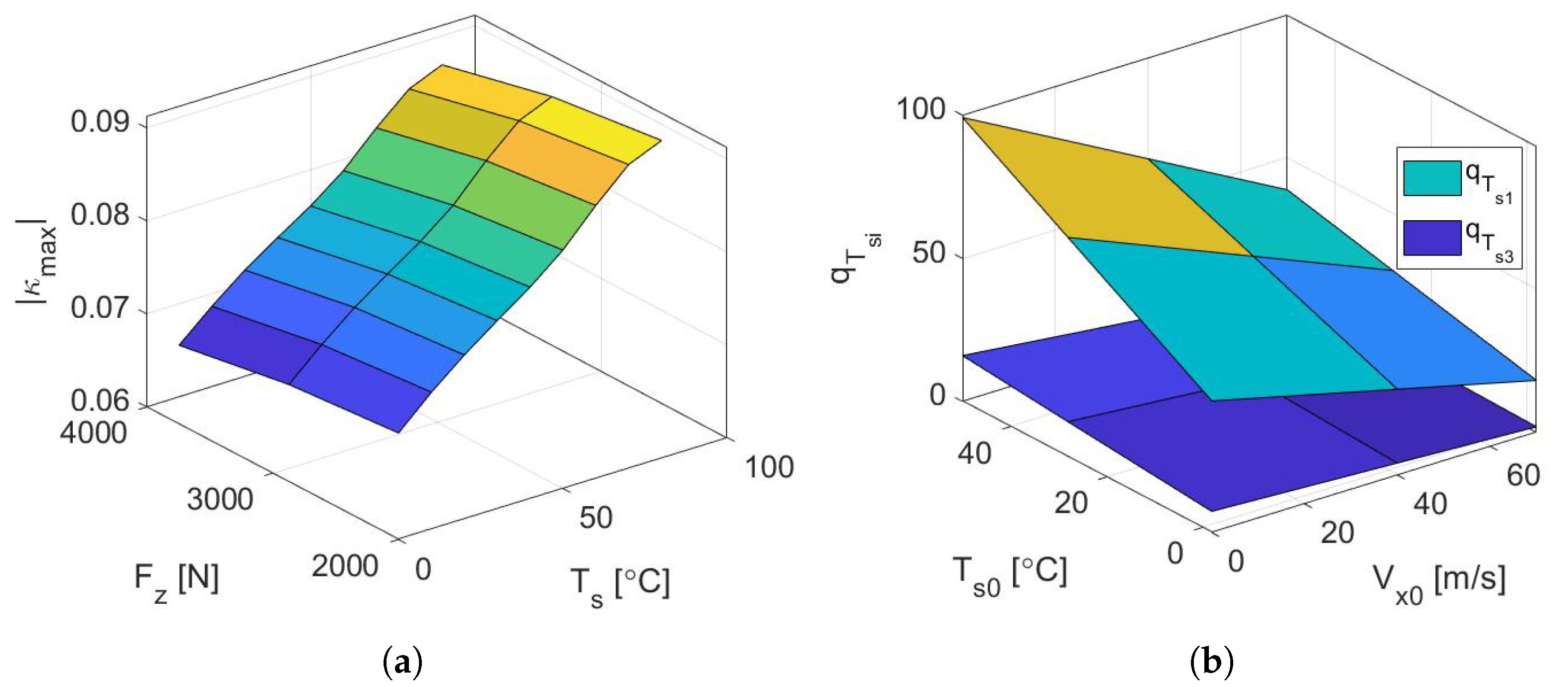
• Maximum tread temperature ($T_{si,max}$): This is the maximum value of the tread surface temperature reached in each test. The subscript i refers to the wheel identity on the car (1, 2, 3, 4)≡($FL$, $FR$, $RL$, $RR$). The higher its value, the more the carcass of the tyre heats up using the heat coming from the tread, of course depending on the initial temperature of the carcass. In such a short braking manoeuvre, an increase in the maximum temperature value can easily depict that there is faster and overall more heating of the tread.

6. Results

6.1. Full-Car Results

The test results mentioned in Section 5 for the full-car are presented. As the total number of tests was 54 (18 tests for each setup), the results are presented in the form of plots of the relative metrics, to keep things comprehensible. For both the metrics, results are presented as percentage changes with respect to the value of Setup A (as discussed in Section 5.2). For the maximum temperature, only the results of the left side of the vehicle are provided, as the differences between left and right tyres were insignificant due to the manoeuvre being symmetric (Section 5).

6.2. Braking Distance

In this section, the braking distance performance is compared with respect to the chosen benchmark setup (Setup A [Pacejka:($\kappa$-contr)]). As previously mentioned, all the values are in percentage change with respect to Setup A.

The results are presented in two plots (Figure 22 and Figure 23), for each initial velocity for the manoeuvre (40 m/s and 70 m/s). Now, comparing Setup B [TempKnwl:($\kappa$-contr)] to Setup A, it is clear that there is improvement in the braking distance as the boundary and initial conditions get hotter and hotter. The maximum improvement was 1%. Additionally, in almost half of the test cases, there was improvement in the braking distance. This clearly shows that giving the controller the knowledge of tyre temperature leads to better performance in the conditions; the parameterisation of Setup A does not match well with the reality. Now, comparing Setup C [TempKnwl:($\kappa$ & $T_s$-contr)] to Setup B, it is clear that as the controller’s energy is also spent on controlling the tyre temperature (making it closer to optimal temperature 70 °C for better grip), there is no improvement in braking distance, although tyre temperature increases more (Figure 24), which could at least provide benefits by heating the tyres faster. A clear reason for this is that an increase in temperature comes at the cost of higher absolute slip than the slip reference, which leads to a decrease in the tyre force (thus, an increase in braking distance), and an increase in grip is not enough to compensate for the lost tyre force. A clear reason for why the temperature is controlled at the cost of slip is that the connection between the input brake torque $T_b$ and the tyre temperature $T_s$ is not direct, but via longitudinal slip $\kappa$. This behaviour is even easier to see in the quarter-car equation (Equation (16)).

For the results of 70 m/s, when comparing Setup B to Setup A, similar improvements can be seen as compared to the results of 40 m/s, but slightly better because the heating (thus, improved grip) at high speeds is higher. Additionally, regarding Setup C compared to Setup B, the loss in braking distance is less as compared to the results for 40 m/s, because at higher velocities (higher friction power) the tyre heating is higher, which leads to more gains in grip due to temperature during the manoeuvre. However, this increased grip is still not enough to compensate for the lost braking force to heat the tyre.

Finally, when comparing Setup C to Setup A, it is clear that braking distance performance was poor until the hot tyre conditions in autumn/spring (Test 5), and after that it showed improvements. However, as will be shown in next section for temperature, Setup C heated the tyre more in all conditions as compared to Setup A and Setup B.

6.3. Temperature Behaviour

Now, looking at the thermal performance ($T_{s1/3,max}$) for both initial velocities (Figure 24 and Figure 25), it is clear that both Setup B and Setup C lead to more heating as compared to Setup A in all the weather conditions (test cases—Figure 20). Although Setup A and Setup B have no means of optimising the tyre’s temperature, Setup B [TempKnwl:($\kappa$-contr)] had better performance as compared to Setup A. The reason for this is that Setup A does not have a temperature-dependent ${\kappa }_{1/3,ref}$ value, which leads to selecting a low value to satisfy all the temperature boundary conditions. Eventually, running with a low absolute slip value leads to less heating.

Finally, comparing Setup C to Setup B—these two setups differ only in the sense that Setup C also tries to optimise the tyre temperature—a huge improvement can be seen in terms of maximum temperature, whereas the maximum gain was 30–35% in Setup C compared to Setup B. As was said before, in the same manoeuvre, achieving a higher maximum temperature value leads to more heating overall. Additionally, looking at the trend, it is clearly visible that the performance is much better in winter conditions as compared to summer, the reason being that the difference between boundary conditions and tyre temperature is very large in summer conditions, which leads to higher convective cooling, and so less heating gains. Finally, when comparing the performance at different initial velocities (Figure 24 and Figure 25), it can be seen that at the higher velocity (70 m/s), the temperature gains were higher overall, the main reason being the fact that the friction power was directly proportional to the velocity.

7. Discussion

As mentioned in Section 5.1 all the simulations were performed in the following environment:

• Plant vehicle model: VI-CarRealTime—in MATLAB/Simulink co-simulation [39].
• Plant tyre model: RIDESuite—in MATLAB/Simulink co-simulation [29,40].
• Controller model: MATLAB/Simulink [41].

In a braking manoeuvre it is expected that the temperature will not rise a lot due to the short duration of the manoeuvre, but in a lap on a race track, for example, such small consistent efforts towards optimising the temp could lead to big improvements throughout the lap/race for a driver.

Even if Setup C is not able to provide decreased braking distance (and only gives an advantage through increased tyre temperature, which can result in quicker tyre heating), it can at least work as a controller (Setup B) that is aware of the changing of the grip factor (Figure 10A) with the temperature and can make better decisions on torque input.

Another weight setting that was tested on the proposed controller (TempKnwl controller) was having the weights on longitudinal slip ${\kappa }_i$ and $T_{si}$ as zero and setting a high weighting for the longitudinal velocity ($q_{V_x}=$ 1 × 10⁵) of the vehicle. This setting is like telling the controller to optimise the slips and temperature by itself to achieve the quickest (optimal) drop in velocity. This setting is called Setup D for convenience. Ideally, the prediction horizon must also be long enough to cover a considerable portion of the braking manoeuvre, which would also enable us to see the slowly (relative to $\kappa$) varying tyre temperature’s effect on grip. However, the SQP solution failed in that case. As a consequence of that, a smaller prediction horizon was tested ($N=2$ and $T_s=0.001$ s $\to T_P=0.002$ s). In this latter case, the SQP was solved successfully, and the brake torques optimally calculated by the controller simply led to longitudinal slips being the ${\kappa }_{i,max}$ for each tyre, which is simply the same as what was achieved in Setup B [TempKnwl:($\kappa$-contr)]. In addition, the computation times of this controller are much longer than those of the Setup B controller, as the controller has to solve a heavier QP as compared to the controller in Setup B. Figure 26 show the time histories of states and control inputs for the 3 setups of full-car NMPC ABS controller in test 5.

8. Conclusions

This work aimed to investigate whether the proposed model-based optimal controller will be able to provide improved performance in terms of longitudinal behaviour by considering the tyre thermodynamics in the controller model. The literature survey revealed NMPC as a novel control technique witnessing great applications in such MIMO systems within vehicle dynamics, as the electronics are improving, and the safety and performance needs of the industry are rising. This systematic and structured control technique was applied to the ABS system with the inclusion of a tyre tread thermal model combined with the famous Pacejka-based tyre force model for the prediction model inside the controller. The chosen tyre tread thermal model for the full-car prediction model was the simplest possible (based on first order dynamics) model that still showed good performance in terms of the main effects that the tyre temperature has on the tyre performance, i.e., grip and stiffness, in a braking manoeuvre.

The final controller was given reference states values and variable weights in the cost function that were functions of the state feedback, thereby improving the performance of the controller and giving it consistent performance throughout various tests. The developed controller was tested with a high-fidelity plant that was composed of a 14-DOF vehicle model coupled with a multi-physical tyre model. The models were parameterised onto a GT-car tyre. Such an excellent parameterisation helped show a realistic impact on controller performance.

The proposed controller was developed in two setups—one that just controls the slip, and the other that controls both slip and the tyre temperature, both fed with the reference slip state for maximum tyre longitudinal force. The braking manoeuvre considered was a pure longitudinal braking manoeuvre where the driver intended to stop the car. Two main metrics were chosen to assess the performance of this high-level controller, the braking distance and the maximum tyre temperature in the manoeuvre. The test results show that when the slip-controller is given the knowledge of tyre temperature, it performs better across the whole range of temperature conditions from winter to summer, whereas the biggest improvements in braking distance were seen to be $1\%$. The improvements in braking distance were seen in almost half of the test cases, but the levels of improvement can be questioned, as they were not huge in terms of absolute distance. A reason for this is directly linked to the fact that the tyre’s longitudinal force characteristics ($F_{x}vs.\kappa$) are relatively flat around the peak, which leads to only a small amount of drop in longitudinal force when the slip value is at least in the vicinity of the peak slip ${\kappa }_{max}$. On the other hand, when the slip and temperature both are controlled, based on the tuning of the controller, so as to not lose a big chunk of braking distance, a maximum of 30–35% improvement in maximum tyre temperature in the manoeuvre was seen. Such improvements in terms of temperature can lead to faster tyre heat-up times while ensuring minimal loss in braking distance, but the real applicability is questionable due to a lack of actuator dynamics being modelled here. Another solution that was expected was that the controller would try to heat the tyre to increase the grip, which would eventually lead to improvements in braking distance, in addition to increased temperature. To extend the current methodology to the lateral vehicle behaviour, the authors have already started to implement and to analyse the impact of the knowledge of the tyre thermal state on the combined tyre–road interaction within the controller model in both HiL and DiL simulation environments, with the aim of implementing the developed techniques directly on real vehicles. To this end, the vehicle plant model has already been tested in concurrent real time hardware, and the control model will be tested in a real-time Speedgoat unit [42], available within the facilities of the research group.

References

- Farroni, F.; Sakhnevych, A.; Timpone, F. An evolved version of thermo racing tyre for real time applications. Lect. Notes Eng. Comput. Sci. 2015, 2218, 1159–1164. [Google Scholar]
- Moore, D.F. Friction and wear in rubbers and tyres. Wear 1980, 61, 273–282. [Google Scholar] [CrossRef]
- Liefferink, R.W.; Hsia, F.C.; Weber, B.; Bonn, D. Friction on ice: How temperature, pressure, and speed control the slipperiness of ice. Phys. Rev. X 2021, 11, 011025. [Google Scholar] [CrossRef]
- Février, P.; Fandard, G. Thermal and mechanical tyre modelling for handling simulation. ATZ Worldw. 2008, 110, 26–31. [Google Scholar] [CrossRef]
- Pretagostini, F.; Ferranti, L.; Berardo, G.; Ivanov, V.; Shyrokau, B. Survey on Wheel Slip Control Design Strategies, Evaluation and Application to Antilock Braking Systems. IEEE Access 2020, 8, 10951–10970. [Google Scholar] [CrossRef]
- Kelly, D.P.; Sharp, R.S. Time-optimal control of the race car: Influence of a thermodynamic tyre model. Veh. Syst. Dyn. 2012, 50, 641–662. [Google Scholar] [CrossRef]
- Perantoni, G.; Limebeer, D.J. Optimal control for a formula one car with variable parameters. Veh. Syst. Dyn. 2014, 52, 653–678. [Google Scholar] [CrossRef] [Green Version]
- Berntorp, K.; Quirynen, R.; Di Cairano, S. Steering of autonomous vehicles based on friction-adaptive nonlinear model-predictive control. In Proceedings of the 2019 American Control Conference (ACC), Philadelphia, PA, USA, 10–12 July 2019; pp. 965–970. [Google Scholar]
- Romano, L.; Johannesson, P.; Bruzelius, F.; Jacobson, B. An enhanced stochastic operating cycle description including weather and traffic models. Transp. Res. Part D Transp. Environ. 2021, 97, 102878. [Google Scholar] [CrossRef]
- Xiong, L.; Yu, Z.; Wang, Y.; Yang, C.; Meng, Y. Vehicle dynamics control of four in-wheel motor drive electric vehicle using gain scheduling based on tyre cornering stiffness estimation. Veh. Syst. Dyn. 2012, 50, 831–846. [Google Scholar] [CrossRef]
- Guo, N.; Lenzo, B.; Zhang, X.; Zou, Y.; Zhai, R.; Zhang, T. A real-time nonlinear model predictive controller for yaw motion optimization of distributed drive electric vehicles. IEEE Trans. Veh. Technol. 2020, 69, 4935–4946. [Google Scholar] [CrossRef] [Green Version]
- Romano, L.; Bruzelius, F.; Hjort, M.; Jacobson, B. Development and analysis of the two-regime transient tyre model for combined slip. Veh. Syst. Dyn. 2022, 8, 1–35. [Google Scholar] [CrossRef]
- Sakhnevych, A. Multiphysical MF-based tyre modelling and parametrisation for vehicle setup and control strategies optimisation. Veh. Syst. Dyn. 2021, 1–22. [Google Scholar] [CrossRef]
- Shim, T.; Ghike, C. Understanding the limitations of different vehicle models for roll dynamics studies. Veh. Syst. Dyn. 2007, 45, 191–216. [Google Scholar] [CrossRef]
- Farroni, F.; Russo, M.; Sakhnevych, A.; Timpone, F. TRT EVO: Advances in real-time thermodynamic tire modeling for vehicle dynamics simulations. Proc. Inst. Mech. Eng. Part D J. Automob. Eng. 2019, 233, 121–135. [Google Scholar] [CrossRef] [Green Version]
- Pacejka, H. Tire and Vehicle Dynamics; Butterworth-Heinemann: Oxford, UK, 2012. [Google Scholar] [CrossRef]
- Harsh, D.; Shyrokau, B. Tire model with temperature effects for formula SAE vehicle. Appl. Sci. 2019, 9, 5328. [Google Scholar] [CrossRef] [Green Version]
- Février, P.; Blanco Hague, O.; Schick, B.; Miquet, C. Advantages of a thermomechanical tire model for vehicle dynamics. ATZ Worldw. 2010, 112, 33–37. [Google Scholar] [CrossRef]
- Hackl, A. Enhanced Tyre Modelling for Vehicle Dynamics Control Systems; Verlag der Technischen Universität Graz: Graz, Austria, 2020; Volume 4, p. 182. [Google Scholar]
- Maniowski, M. Optimisation of driver actions in RWD race car including tyre thermodynamics. Veh. Syst. Dyn. 2016, 54, 526–544. [Google Scholar] [CrossRef] [Green Version]
- Tremlett, A.J.; Limebeer, D.J. Optimal tyre usage for a Formula One car. Veh. Syst. Dyn. 2016, 54, 1448–1473. [Google Scholar] [CrossRef]
- West, W.; Limebeer, D. Optimal tyre management for a high-performance race car. Veh. Syst. Dyn. 2020, 60, 1–19. [Google Scholar] [CrossRef]
- Calabrese, F.; Baecker, M.; Galbally, C.; Gallrein, A. A Detailed Thermo-Mechanical Tire Model for Advanced Handling Applications. SAE Int. J. Passeng. Cars Mech. Syst. 2015, 8, 501–511. [Google Scholar] [CrossRef]
- De Rosa, R.; Di Stazio, F.; Giordano, D.; Russo, M.; Terzo, M. ThermoTyre: Tyre temperature distribution during handling manoeuvres. Veh. Syst. Dyn. 2008, 46, 831–844. [Google Scholar] [CrossRef]
- Farroni, F.; Giordano, D.; Russo, M.; Timpone, F. TRT: Thermo racing tyre a physical model to predict the tyre temperature distribution. Meccanica 2014, 49, 707–723. [Google Scholar] [CrossRef] [Green Version]
- Capra, D.; Farroni, F.; Sakhnevych, A.; Salvato, G.; Sorrentino, A.; Timpone, F. On the Implementation of an Innovative Temperature-Sensitive Version of Pacejka’s MF in Vehicle Dynamics Simulations. In Proceedings of the XXIV AIMETA Conference, Rome, Italy, 15–19 September 2019; Springer: Berlin/Heidelberg, Germany, 2019; pp. 1084–1092. [Google Scholar]
- Frasch, J.V.; Gray, A.; Zanon, M.; Ferreau, H.J.; Sager, S.; Borrelli, F.; Diehl, M. An auto-generated nonlinear MPC algorithm for real-time obstacle avoidance of ground vehicles. In Proceedings of the 2013 European Control Conference, ECC 2013, Zurich, Switzerland, 17–19 July 2013; pp. 4136–4141. [Google Scholar] [CrossRef]
- Ayub, A.; Wahab, H.A.; Balubaid, M.; Mahmoud, S.; Ali, M.R.; Sadat, R. Analysis of the nanoscale heat transport and Lorentz force based on the time-dependent Cross nanofluid. Eng. Comput. 2022, 1–20. [Google Scholar] [CrossRef]
- Farroni, F.; Sakhnevych, A. Tire multiphysical modeling for the analysis of thermal and wear sensitivity on vehicle objective dynamics and racing performances. Simul. Model. Pract. Theory 2022, 117, 102517. [Google Scholar] [CrossRef]
- Farroni, F. TRICK-Tire/Road Interaction Characterization & Knowledge-A tool for the evaluation of tire and vehicle performances in outdoor test sessions. Mech. Syst. Signal Process. 2016, 72, 808–831. [Google Scholar]
- Petersen, I.; Johansen, T.A.; Kalkkuhl, J.; Ludemann, J. Gain-scheduled wheel slip reset control in automotive brake systems. In Proceedings of the 2001 European Control Conference, ECC 2001, Porto, Portugal, 4–7 September 2001; pp. 606–611. [Google Scholar] [CrossRef]
- Alirezaei, M.; Kanarachos, S.; Scheepers, B.; Maurice, J.P. Experimental evaluation of optimal Vehicle Dynamic Control based on the State Dependent Riccati Equation technique. In Proceedings of the 2013 American Control Conference, Washington, DC, USA, 17–19 June 2013; pp. 408–412. [Google Scholar] [CrossRef]
- Wachter, E.; Alirezaei, M.; Bruzelius, F.; Schmeitz, A. Path control in limit handling and drifting conditions using State Dependent Riccati Equation technique. Proc. Inst. Mech. Eng. Part D J. Automob. Eng. 2020, 234, 783–791. [Google Scholar] [CrossRef]
- Menon, P.; Lam, T.; Crawford, L.; Cheng, V. Real-time computational methods for SDRE nonlinear control of missiles. In Proceedings of the 2002 American Control Conference (IEEE Cat. No. CH37301), Anchorage, AK, USA, 8–10 May 2002; Volume 1, pp. 232–237. [Google Scholar]
- Press, W.H.; Teukolsky, S.A.; Vetterling, W.T.; Flannery, B.P. Numerical Recipes with Source Code CD-ROM, 3rd Edition: The Art of Scientific Computing; Cambridge University Press: Cambridge, UK, 2007. [Google Scholar]
- Kunnappillil Madhusudhanan, A.; Corno, M.; Bonsen, B.; Holweg, E. Solving algebraic riccati equation real time for integrated vehicle dynamics control. In Proceedings of the American Control Conference, Montreal, QC, Canada, 27–29 June 2012; pp. 3593–3598. [Google Scholar] [CrossRef]
- Bryson, A.; Ho, Y. Applied Optimal Control: Optimization, Estimation, and Control; Blaisdell Pub. Co.: Waltham, MA, USA, 1969. [Google Scholar]
- Itik, M.; Salamci, M.U.; Banks, S.P. SDRE optimal control of drug administration in cancer treatment. Turk. J. Electr. Eng. Comput. Sci. 2010, 18, 715–729. [Google Scholar] [CrossRef]
- Available online: https://www.vi-grade.com/en/products/vi-carrealtime (accessed on 5 May 2022).
- Available online: https://www.megaride.eu/ (accessed on 5 May 2022).
- Available online: https://www.mathworks.com/ (accessed on 5 May 2022).
- Available online: https://www.speedgoat.com/ (accessed on 5 May 2022).