A New Coupled Approach for Enthalpy Pumping Consideration in a Free Piston Stirling Engine (FPSE)

 , , and
Abstract
:1. Introduction
1.1. Literature Review
1.2. Contribution
- -
- The enthalpy pumping is studied in a Free Piston Stirling Engine.
- -
- The enthalpy pumping idea is developed based on a precise nonlinear dynamic model of an FPSE [15].
- -
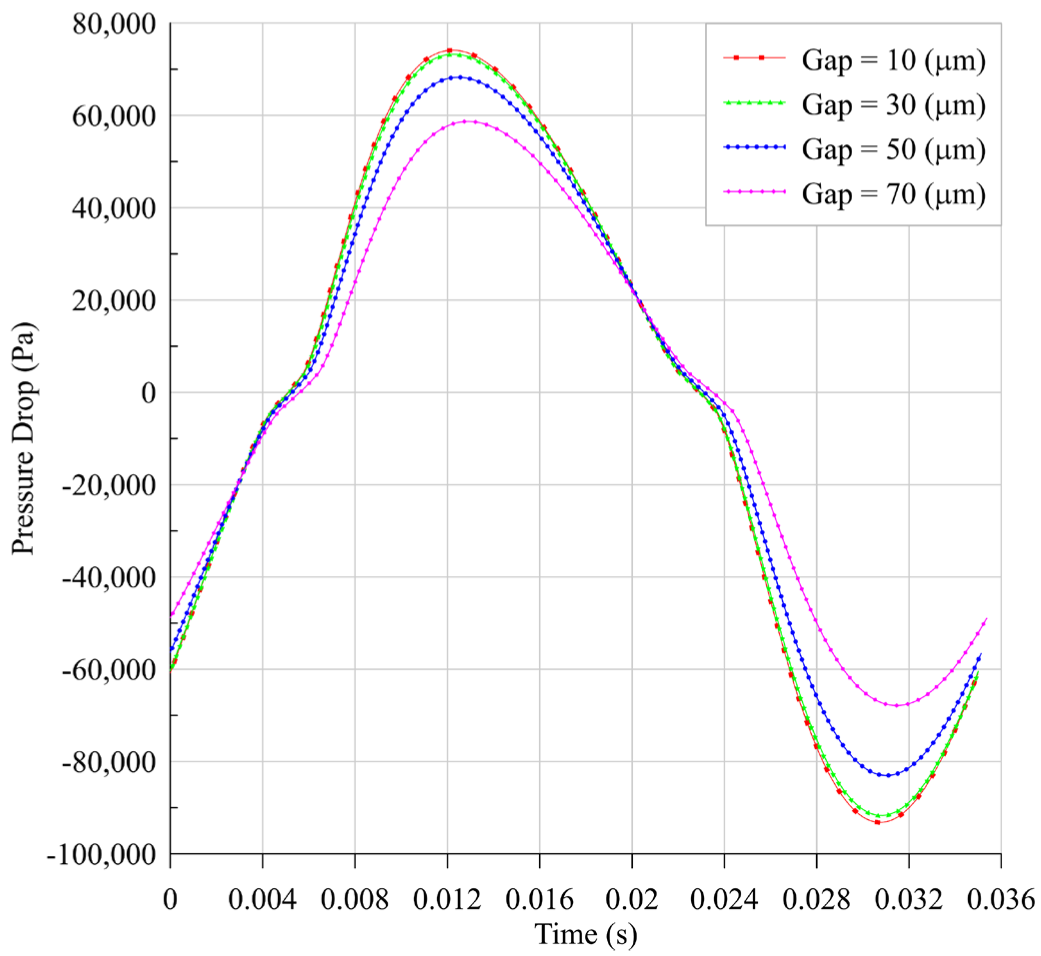
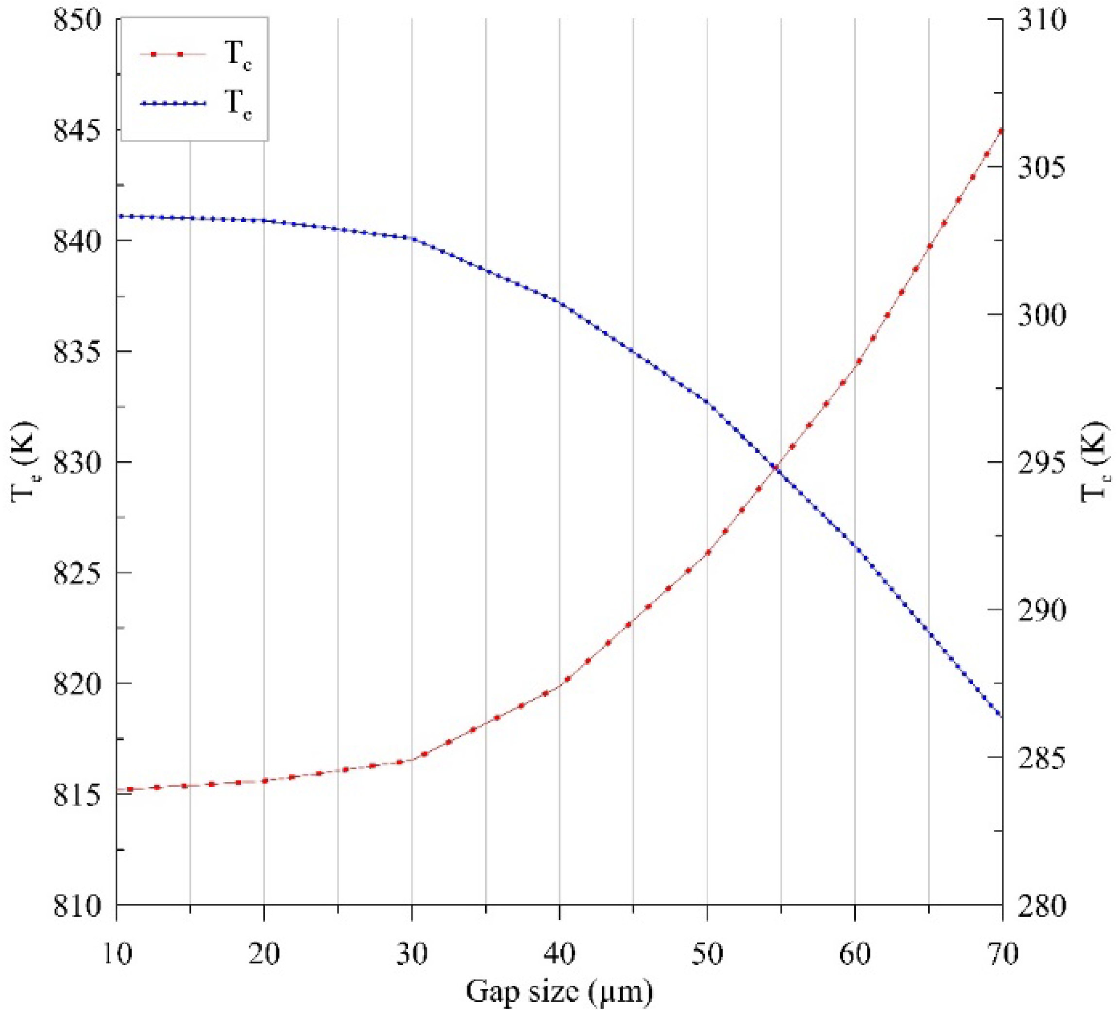
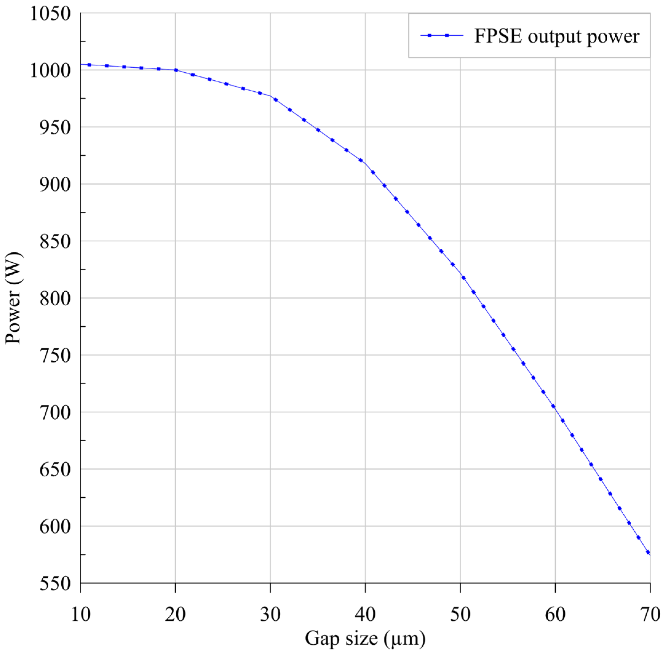
- The real-time enthalpy pumping effect on the FPSE behavior through a coupled model is studied taking into account the following parameters: pressure difference between expansion and compression spaces, mean temperatures of expansion and compression spaces, and output power.
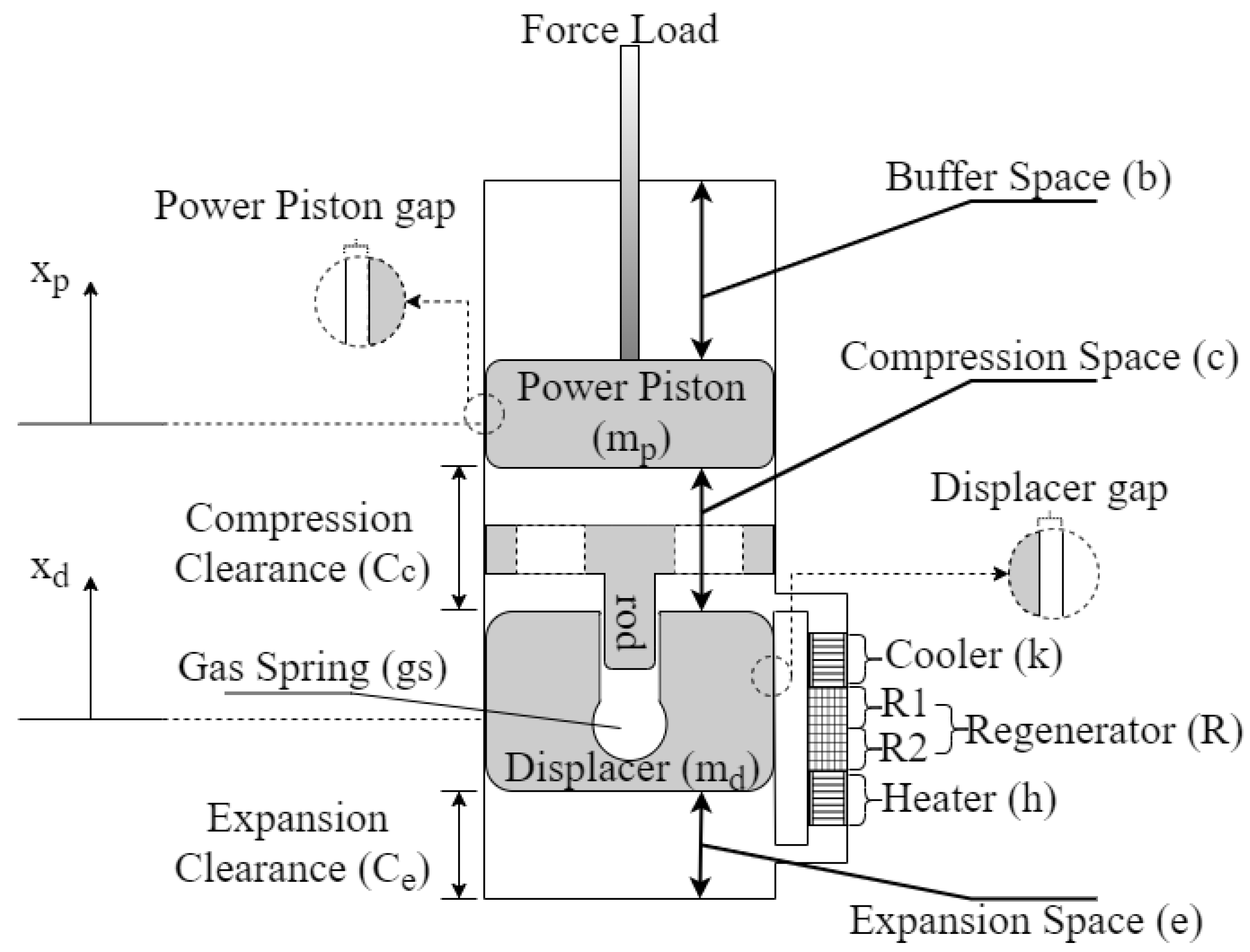
2. Problem Formulation
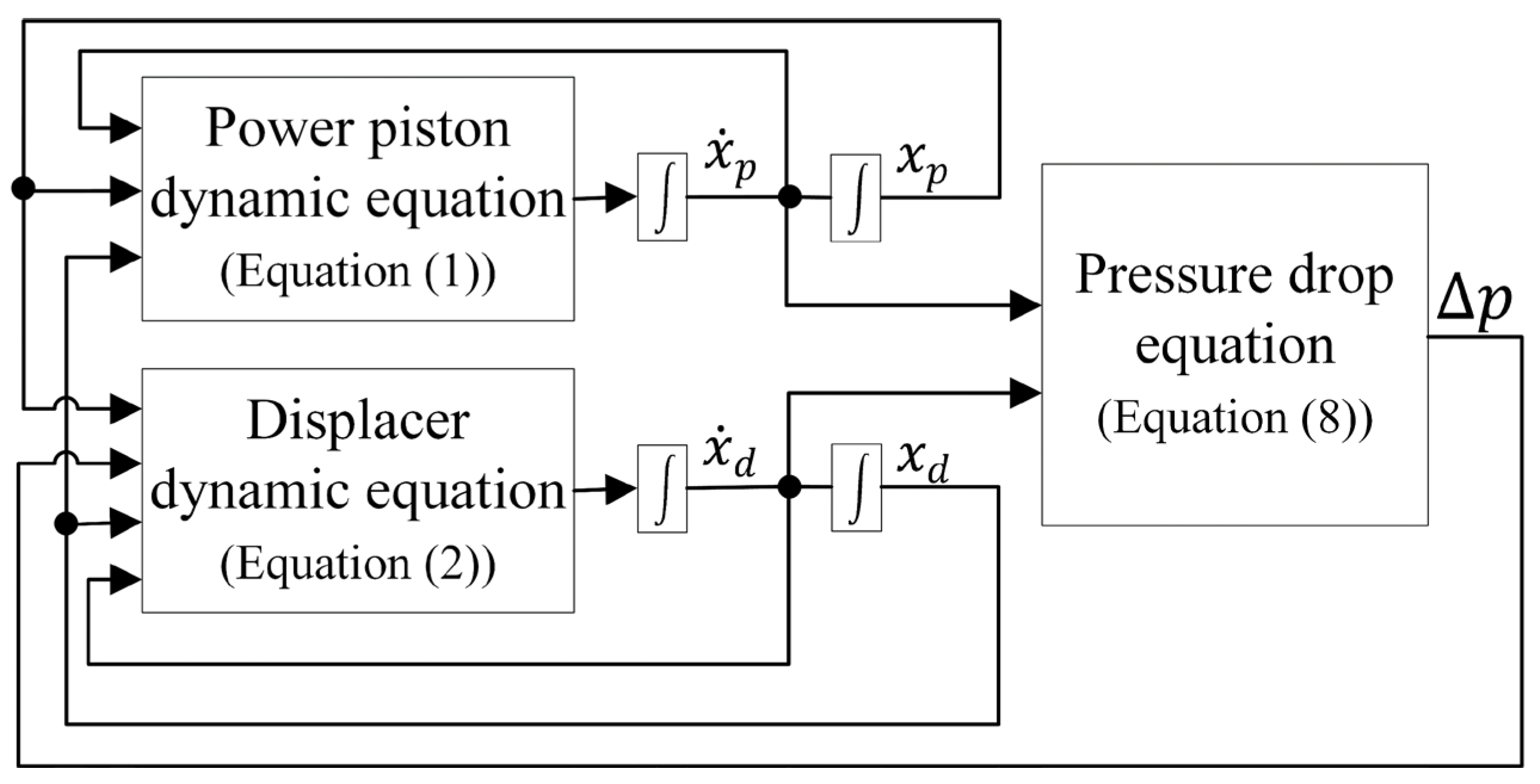
3. FPSE Dynamic Model
3.1. Methodology
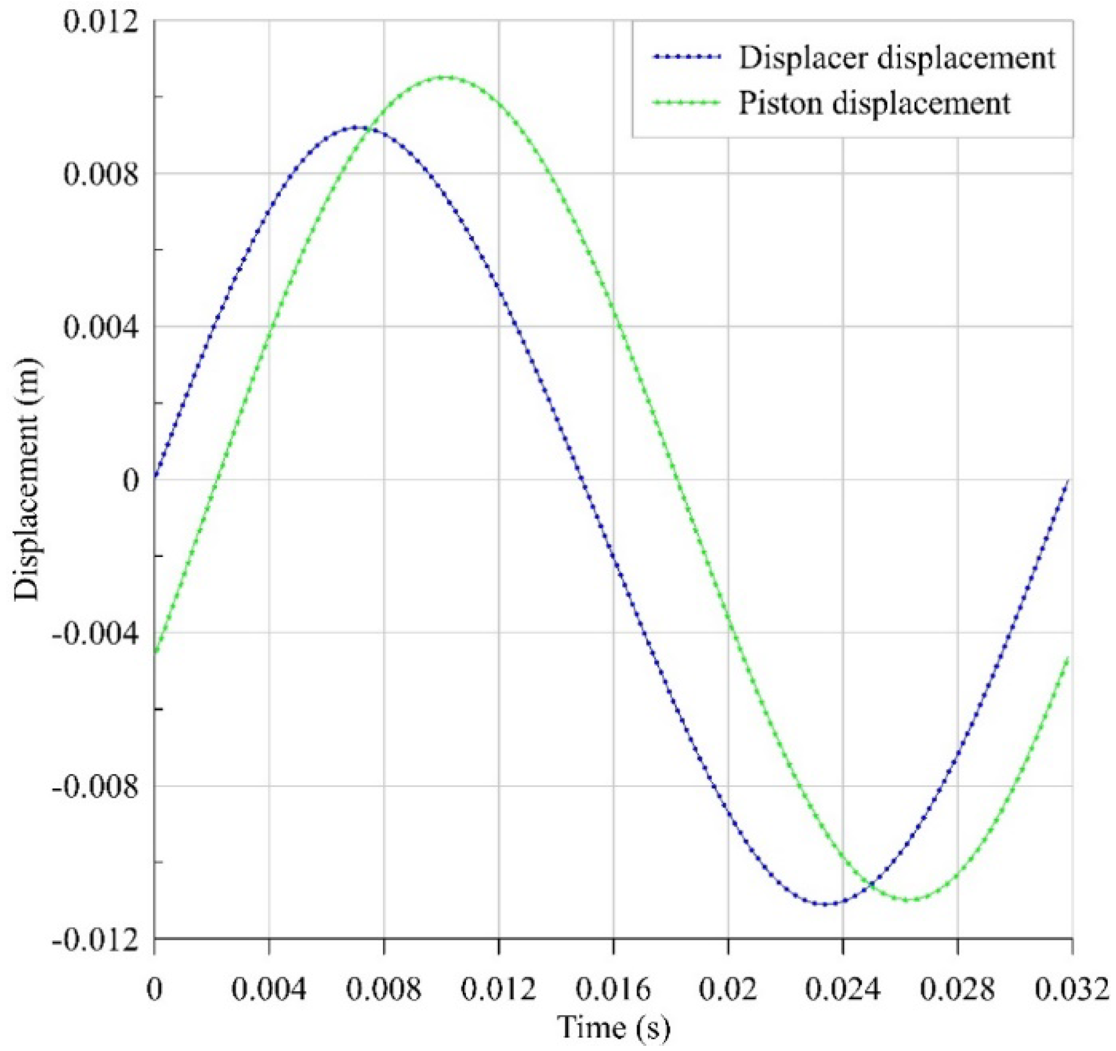
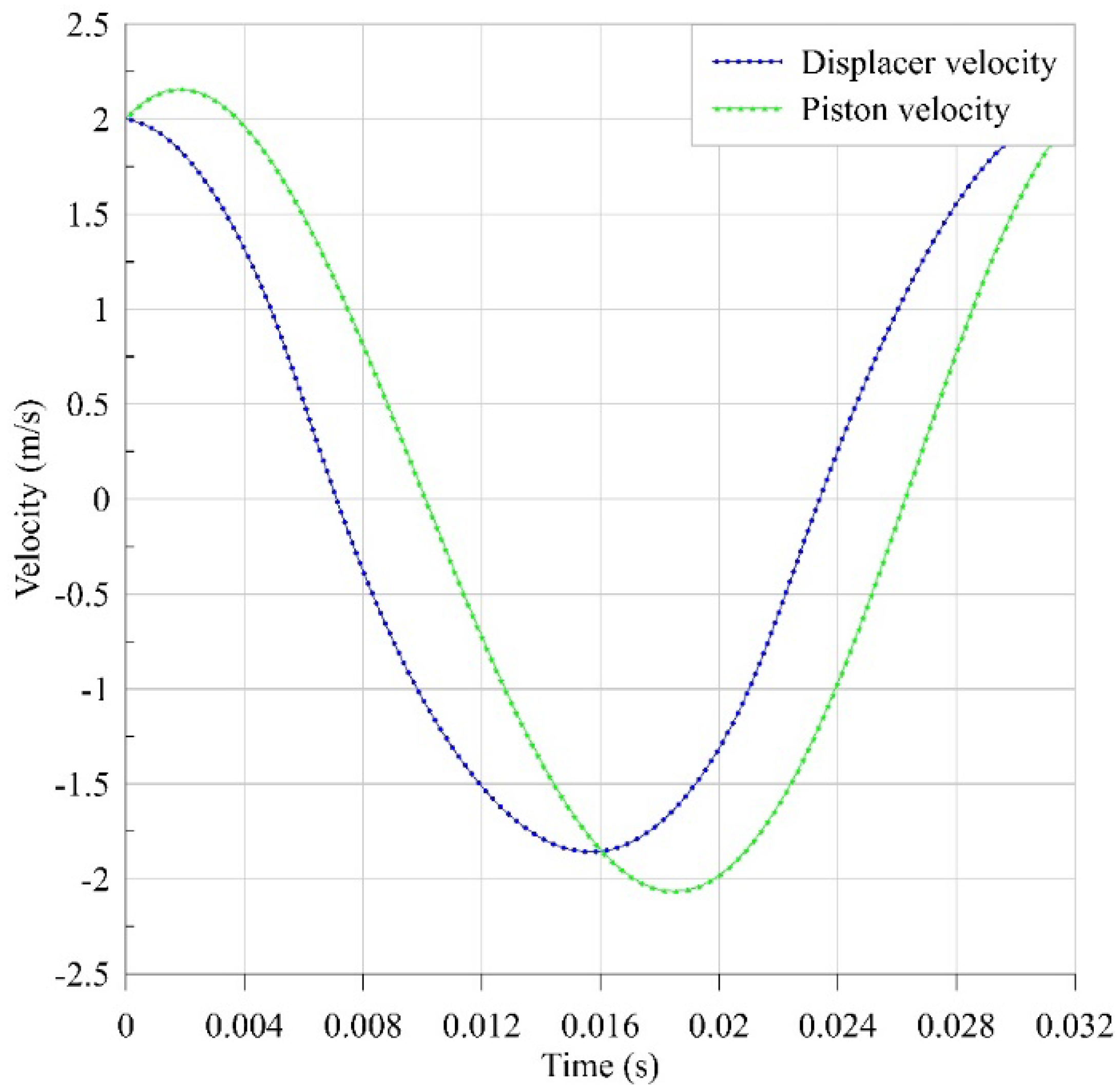
3.2. Results
4. Enthalpy Pumping through Displacer Gap
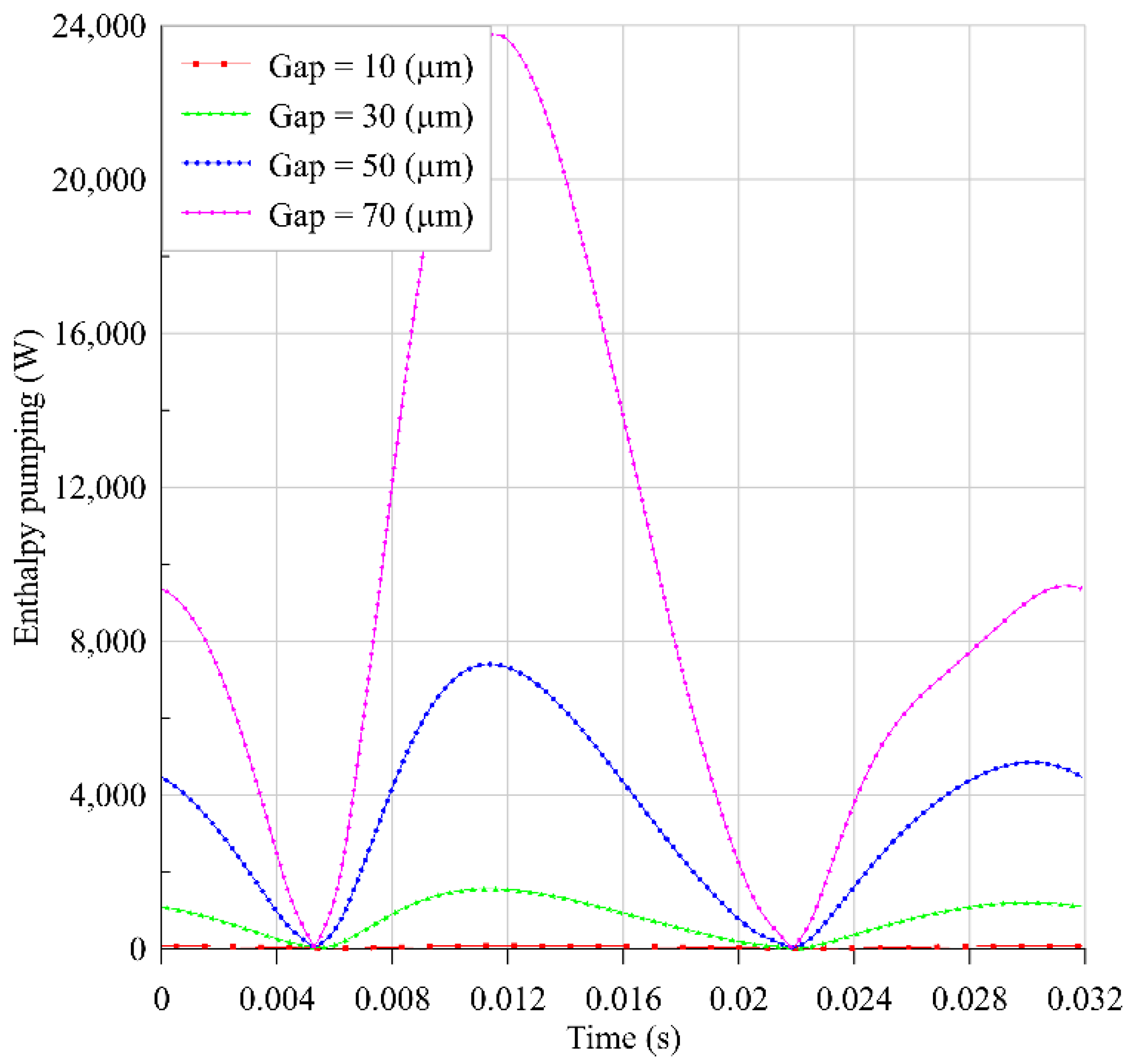
4.1. Decoupled Model
4.1.1. Methodology
4.1.2. Results
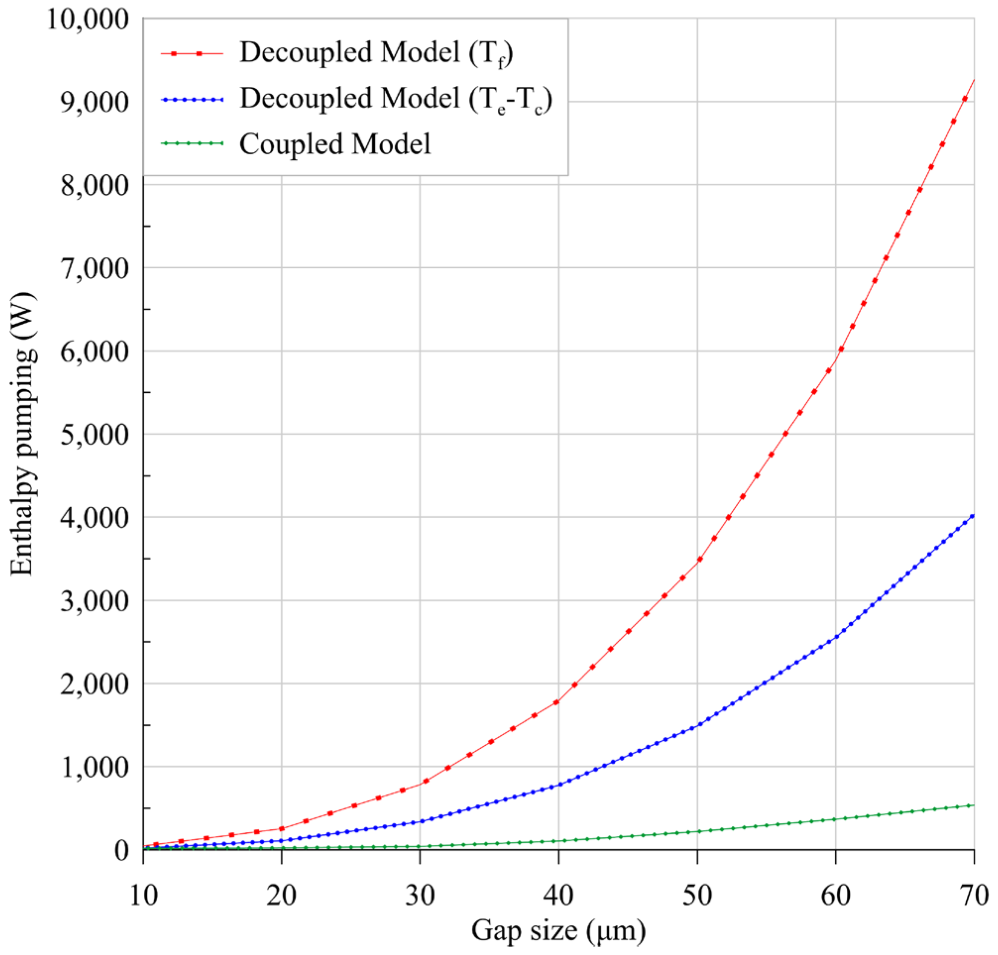
4.2. Coupled Model
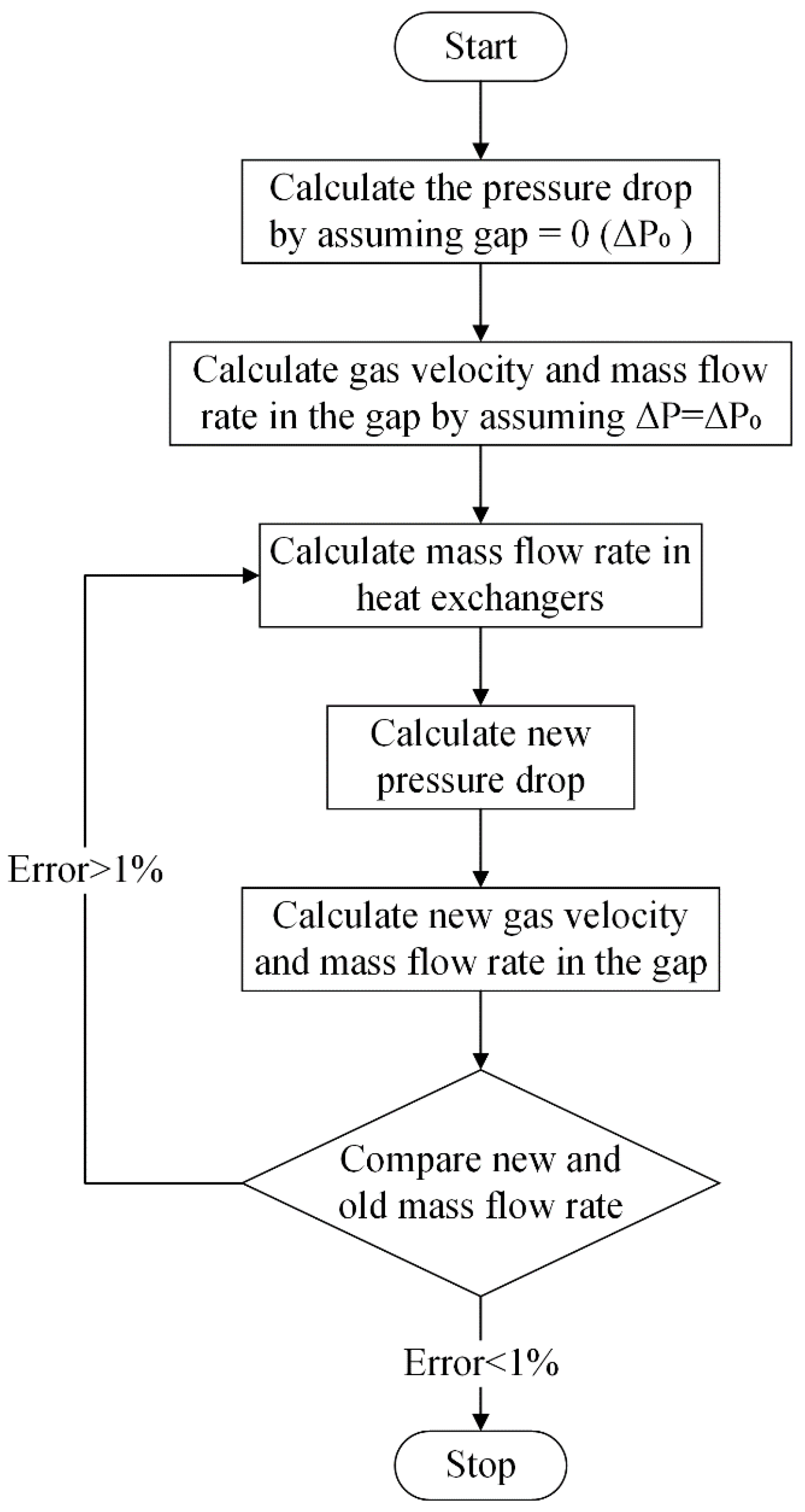
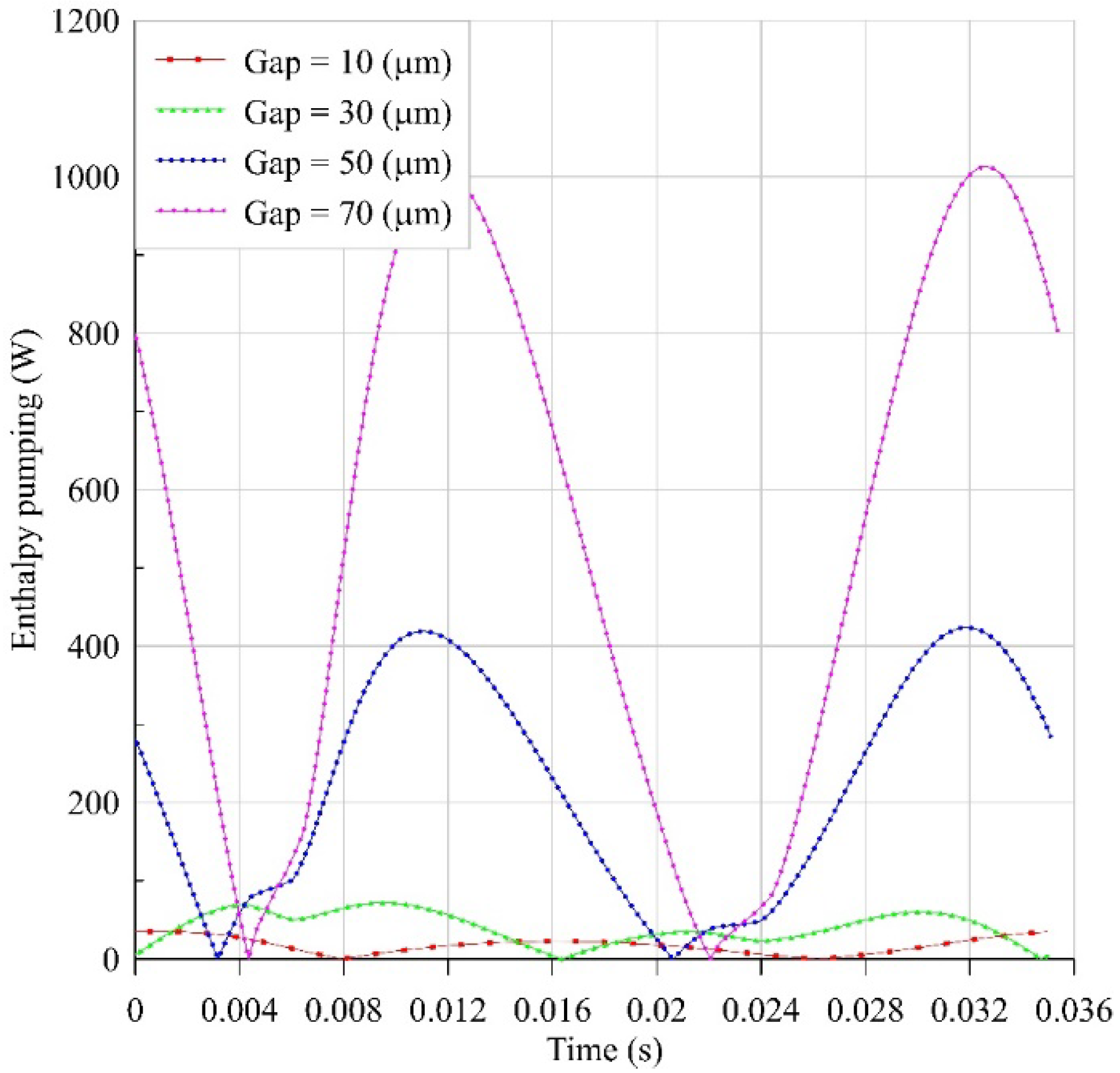
4.2.1. Methodology
4.2.2. Results
5. Conclusions
Author Contributions
Funding
Conflicts of Interest
Nomenclature
| Area, m2 | Acceleration, m/s2 | ||
| Clearance, m | Axis | ||
| Darcy friction factor | Greek symbols | ||
| Specific heat capacity at constant pressure, J/( kg·K) | Thermal diffusivity, m2/s | ||
| Specific heat capacity at constant volume, J/( kg·K) | Isochoric thermal pressure coefficient, 1/K | ||
| Diameter, m | Temperature variation, K/m | ||
| Force, N | Specific heat ratio | ||
| Enthalpy rate, W | Thickness, m | ||
| Thermal Conductivity, W/(m·K) | Dynamic viscosity, Pa.s | ||
| Length, m | Kinematic viscosity, m2/s | ||
| Mass, kg | Density, kg/m3 | ||
| Pressure, Pa | Index and exponent | ||
| Heat transfer rate, W | Time average | ||
| Gas constant, Radius, m | Oscillating part | ||
| Radius, m | Buffer | ||
| Reynolds number | Compression, Cylinder | ||
| Temperature, K | Displacer | ||
| Time, s | Expansion | ||
| Gas velocity, m/s | Flow | ||
| Volume, m3 | Gas spring | ||
| Volumetric rate, m3/s | Heater | ||
| Work rate, W | Cooler | ||
| Maximum stroke, m | Power piston | ||
| Displacement, m | Regenerator | ||
| Piston velocity, m/s | Wire | ||
References
- Zare, S.; Tavakolpour-Saleh, A.R. Frequency-Based Design of a Free Piston Stirling Engine Using Genetic Algorithm. Energy 2016, 109, 466–480. [Google Scholar] [CrossRef]
- Wang, K.; Sanders, S.R.; Dubey, S.; Choo, F.H.; Duan, F. Stirling Cycle Engines for Recovering Low and Moderate Temperature Heat: A Review. Renew. Sustain. Energ. Rev. 2016, 62, 89–108. [Google Scholar] [CrossRef] [Green Version]
- Sauer, J.; Kuehl, H.D. Theoretically and Experimentally Founded Simulation of the Appendix Gap in Regenerative Machines. Appl. Therm. Eng. 2020, 166, 114530. [Google Scholar] [CrossRef]
- Urieli, I.; Berchowitz, D. Stirling Cycle Engine Analysis; Adam Hilger Ltd.: Bristol, UK, 1984; ISBN 978-0996002196. [Google Scholar]
- Redlich, R.W.; Berchowitz, D.M. Linear Dynamics of Free-Piston Stirling Engines. Proc. Inst. Mechan. Eng. Part Power Proc. Eng. 1985, 199, 203–213. [Google Scholar] [CrossRef]
- Walker, G.; Senft, J.R. Free-Piston Stirling Engines. In Free Piston Stirling Engines; Springer: Berlin/Heidelberg, Germany, 1985; pp. 23–99. [Google Scholar]
- Mabrouk, M.T.; Kheiri, A.; Feidt, M. Displacer Gap Losses in Beta and Gamma Stirling Engines. Energy 2014, 72, 135–144. [Google Scholar] [CrossRef]
- Mabrouk, M.T.; Kheiri, A.; Feidt, M. Effect of Leakage Losses on the Performance of a β Type Stirling Engine. Energy 2015, 88, 111–117. [Google Scholar] [CrossRef]
- Rios, P.A. An Approximate Solution To the Shuttle Heat-Transfer Losses in a Reciprocating Machine. J. Eng. Power 1971, 93, 177–182. [Google Scholar] [CrossRef]
- Berchowitz, D.M. Stirling Cycle Engine Design and Optimisation. Ph.D. Thesis, University of the Witwatersrand, Johannesburg, South Africa, 1986. [Google Scholar]
- Baik, J.H.; Chang, H.M. An Exact Solution for Shuttle Heat Transfer. Cryogenics 1995, 35, 9–13. [Google Scholar] [CrossRef]
- Chang, H.M.; Park, D.J.; Jeong, S. Effect of Gap Flow on Shuttle Heat Transfer. Cryogenics 2000, 40, 159–166. [Google Scholar] [CrossRef]
- Kotsubo, V.; Swift, G. Thermoacoustic Analysis of Displacer Gap Loss in a Low Temperature Stirling Cooler. In Proceedings of the AIP Conference Proceedings; American Institute of Physics: College Park, MA, USA, 2006; Volume 823, pp. 353–360. [Google Scholar]
- Pfeiffer, J.; Kuehl, H.D. New Analytical Model for Appendix Gap Losses in Stirling Cycle Machines. J. Therm. Heat Transf. 2016, 30, 288–300. [Google Scholar] [CrossRef]
- Majidniya, M.; Boileau, T.; Remy, B.; Zandi, M. Nonlinear Modeling of a Free Piston Stirling Engine Combined with a Permanent Magnet Linear Synchronous Machine. Appl. Therm. Eng. 2020, 165, 114544. [Google Scholar] [CrossRef]
- Majidniya, M.; Boileau, T.; Remy, B.; Zandi, M. Performance Simulation by a Nonlinear Thermodynamic Model for a Free Piston Stirling Engine with a Linear Generator. Appl. Therm. Eng. 2021, 184, 116128. [Google Scholar] [CrossRef]
- Majidniya, M.; Boileau, T.; Benjamin, R.; Zandi, M. Modélisation Thermo-Électrique d’un Moteur Stirling à Piston Libre et d’une Machine Synchrone Linéaire à Aimant Permanent Avec Sa Commande. In Proceedings of the congrès annuel de la Société Française de Thermique, Nantes, Toulouse, France, 3–6 June 2019. [Google Scholar]
- Schreiber, J. Testing and Performance Characteristics of a 1-Kw Free Piston Stirling Engine. NASA Technical Memorandum. 1983. Available online: https://ntrs.nasa.gov/citations/19830016765 (accessed on 20 March 2022).
- Batchelor, C.K.; Batchelor, G.K. An Introduction to Fluid Dynamics; Cambridge University Press: Cambridge, UK, 1959. [Google Scholar]


| For Heater and Cooler: | < 2000 | |
| > 2000 | ||
| For Regenerator: | < 60 | |
| 60 < Re < 1000 | ||
| > 1000 |
| 814.3 K | 0.2362 cm | 1.861 cm | |||
| 322.8 K | 0.00889 cm | 2615 cm3 | |||
| 71 bars | 7.92 cm | 37.97 cm3 | |||
| 75.9% | 18.34 cm | 56.37 cm3 | |||
| 0.426 kg | 6.44 cm | 115.2 cm | |||
| 6.2 kg | 1.4898 cm2 | 50.8 mm 376 mm | |||
| 5.718 cm | 2.6163 cm2 | 135 | |||
| 5.67 cm | 8.745 cm2 | 4.20 cm | |||
| 1.663 cm | 1.83 cm | 4.04 cm |
| Frequency (Hz) | Output Power (kW) | |||
|---|---|---|---|---|
| Exp. Results [4] | 30 | −42.5 | 1.06 | 1.00 |
| Present Model | 31.25 | −33.75 | 0.945 | 1.005 |
Publisher’s Note: MDPI stays neutral with regard to jurisdictional claims in published maps and institutional affiliations. |
© 2022 by the authors. Licensee MDPI, Basel, Switzerland. This article is an open access article distributed under the terms and conditions of the Creative Commons Attribution (CC BY) license (https://creativecommons.org/licenses/by/4.0/).
Share and Cite
Majidniya, M.; Mabrouk, M.T.; Kheiri, A.; Remy, B.; Boileau, T. A New Coupled Approach for Enthalpy Pumping Consideration in a Free Piston Stirling Engine (FPSE). Appl. Mech. 2022, 3, 339-359. https://doi.org/10.3390/applmech3020021
Majidniya M, Mabrouk MT, Kheiri A, Remy B, Boileau T. A New Coupled Approach for Enthalpy Pumping Consideration in a Free Piston Stirling Engine (FPSE). Applied Mechanics. 2022; 3(2):339-359. https://doi.org/10.3390/applmech3020021
Chicago/Turabian StyleMajidniya, Mahdi, Mohamed Tahar Mabrouk, Abdelhamid Kheiri, Benjamin Remy, and Thierry Boileau. 2022. "A New Coupled Approach for Enthalpy Pumping Consideration in a Free Piston Stirling Engine (FPSE)" Applied Mechanics 3, no. 2: 339-359. https://doi.org/10.3390/applmech3020021
APA StyleMajidniya, M., Mabrouk, M. T., Kheiri, A., Remy, B., & Boileau, T. (2022). A New Coupled Approach for Enthalpy Pumping Consideration in a Free Piston Stirling Engine (FPSE). Applied Mechanics, 3(2), 339-359. https://doi.org/10.3390/applmech3020021