Identification of Fractional Damping Parameters in Structural Dynamics Using Polynomial Chaos Expansion

Abstract

In order to analyze the dynamics of a structural problem accurately, a precise model of the structure, including an appropriate material description, is required. An important step within the modeling process is the correct determination of the model input parameters, e.g., loading conditions or material parameters. An accurate description of the damping characteristics is a complicated task, since many different effects have to be considered. An efficient approach to model the material damping is the introduction of fractional derivatives in the constitutive relations of the material, since only a small number of parameters is required to represent the real damping behavior. In this paper, a novel method to determine the damping parameters of viscoelastic materials described by the so-called fractional Zener material model is proposed. The damping parameters are estimated by matching the Frequency Response Functions (FRF) of a virtual model, describing a beam-like structure, with experimental vibration data. Since this process is generally time-consuming, a surrogate modeling technique, named Polynomial Chaos Expansion (PCE), is combined with a semi-analytical computational technique, called the Numerical Assembly Technique (NAT), to reduce the computational cost. The presented approach is applied to an artificial material with well defined parameters to show the accuracy and efficiency of the method. Additionally, vibration measurements are used to estimate the damping parameters of an aluminium rotor with low material damping, which can also be described by the fractional damping model.

1. Introduction

In modern engineering applications, advanced materials and material combinations are used to tackle vibration problems. In order to analyze such structures with a virtual model, an accurate representation of the structure, including geometric details, material characteristics, loading conditions etc., is required. While the geometric description is generally available from CAD data, the material parameters of the model are often unknown and have to be determined by comparison with measurement results.

For an appropriate description of the real structure, viscoelastic material behavior is often required. While a perfectly elastic material has three assumptions, namely the linearity, the simultaneity, and the unique equilibrium value between the stress and strain [1], viscoelastic material models only require linearity [1]. Rheological models for these materials can be illustrated as combinations of springs and dampers [2]. In the present paper, the fractional Zener model is used, which is a modification of the traditional Zener model presented in [3]. While the classical Zener model contains two springs and a dashpot [4], the introduction of fractional calculus leads to a modification of the dashpot behavior, see, e.g., [4,5], and an additional fourth parameter, the fractional-order of the time derivative, is introduced [6]. This modification allows for the representation of real materials with a low number of parameters [6].

A possibility to estimate the parameters in the material model is through a minimization of the error between a numerical model and measurements. Different experimental setups are available to generate reference data for the minimization process. Quasi-static methods, such as the creep test and the relaxation test, analyze the behavior of the materials to an impulsive loading over a long time [1], while dynamic methods consider the response to varying loads. According to [7], the dynamic methods can further be categorized into the Dynamic Mechanical Analysis (DMA) [8] and vibration tests [9]. Several other techniques are listed in [9], with a special focus on the estimation of damping.

The analysis of the material behavior by DMA is based on the measurement of the amplitude and the lag in the stress–strain relation caused by an oscillating force [8]. Then, the parameters of the model, such as the modulus and the damping, can be calculated [8]. In [10], the viscoelastic material parameters of synthetic rubber are estimated by DMA. The damping of the test object is described by a Maxwell model, where two different specifications are compared [10]. First, a series Maxwell setup containing 12 components and second, a fractional derivative model containing a springpot element instead of the dashpot is analyzed [10]. In [11], a unidirectional glass fibre-reinforced epoxy is investigated, where a three-point bending test including the effect of different temperatures of the test object is applied.

DMA leads to very good estimates for the material parameters, but expensive test equipment is required [12] and the method is limited to low frequencies [7]. Alternatively, vibration tests can be used to estimate the material properties. In [7], a bare beam and a sandwich structure are analyzed by shaker tests. The Frequency Response Function (FRF) curve is used in a model updating process applying the amplitude correlation coefficient [7]. The results are compared to those of DMA and show that the vibration test was found superior [7]. In [12], a setup containing two beams with different lengths is analyzed by impact hammer tests. The response is measured by an acceleration sensor and the complex Young’s modulus is estimated, based on the comparison of a calculated FRF of the beam and the measured response [12].

Comparing the measured FRF curves with numerical data is also used by other researchers, like in [13,14,15]. In [13], isotropic and orthotropic material parameters are estimated from bending tests. Finite element (FE) simulations predict the viscoelastic material behavior and the Levenberg–Marquard algorithm is used for the estimation of the best fitting parameters [13]. In [14], a finite element model is applied to describe the test object containing a beam with a layer of viscoelastic damping material in a clamped-free boundary condition. The FRF curves are used to extract the values of the eigenfrequencies and amplitudes at these eigenfrequencies for the Parameter Identification Process [14]. A two-step minimization is applied to estimate the best fitting parameters in combination with a parameter sensitivity analysis [14]. In [15], a viscoelastic composite plate is investigated. Amplitude values at the resonance frequency and close to the resonance frequency are used to fit the parameters [15].

Generally, simple objects such as beams or plates are used in the process of material identification, since the modeling is less involved and the measurements are easier to conduct. Nowadays, various methods exist to solve one-dimensional structural problems, such as the Transfer Matrix Method, the Dynamic Stiffness Method or the Green function method [16]. These methods involve a frequency-dependent system matrix that needs to be solved numerically [16]. In the present paper, a (semi-)analytical method, named Numerical Assembly Technique (NAT), is used to describe one-dimensional beam structures. The method was introduced by Wu and Chou [17] in 1999. NAT subdivides the beam structure into segments that contain a constant cross-section and constant material parameters [16]. The homogeneous governing equations of the uniform beam segments are solved analytically and the resulting solutions are used to fit the boundary and interface conditions [16].

Generally, the minimization process for the parameter identification requires numerous evaluations of the numerical models, which is a time-consuming process. In order to raise the efficiency of the Parameter Identification Process, the numerical model can be replaced by a surrogate model. Several surrogate modeling techniques exist, such as the Artificial Neural Network [18,19,20,21], parametric Reduced Order Model [22], the Response Surface Method [23] or the Polynomial Chaos Expansion (PCE) [24,25,26,27,28]. In [18,19], a viscoelastic cylinder coated by water is analyzed and the complex Young’s modulus is estimated. An Artificial Neural Network is used as a surrogate model. In [20,21], a laminated structure is analyzed. The FRF curve gives the reference values and an Artificial Neural Network is used for the surrogate modeling process [20,21]. A Bayesian approach is applied for the estimation process [20,21]. In [22], a reduction in the computational time is achieved by the reduction in the order of the model in order to efficiently estimate the complex shear modulus. In [23], a Response Surface Method is used to describe the reference values based on the storage modulus and the loss factor. In [24], a frictional system is analyzed and the Polynomial Chaos Expansion is used as a surrogate modeling technique. In [25,26], composite plates are analyzed and, based on the deviation of the results, the input parameters are chosen to describe the polynomial basis. In [27,28], a special combination of the Polynomial Chaos Expansion to estimate the material parameters [27] and bearing stiffness parameters of a test rig [28] is shown. The used method is called Polynomial Chaos Kriging and uses the Polynomial Chaos Expansion for a global system description and the Kriging method for the interpolation of local values [29].

In the present work, PCE is used, which approximates the complex numerical model by orthonormal polynomials to reduce the computational load. PCE is based on the concept of Wiener [30] and has been extended by Cameron and Martin [31] using non-linear functions defined by a Fourier–Hermite series [32,33,34]. Many refinements and new fields of applications for PCE have been investigated, which are summarized by Ghanem and Spanos [32]. The aim of PCE is to span a space based on a polynomial basis and correlating coefficients in order to build a surrogate model [34]. Depending on the distribution of the input parameters, different polynomials can be applied, as listed in, e.g., [33].

The outline of the paper reads as follows: In Section 2, the two numerical methods are explained, which build the basis for the Parameter Identification Process (PIP). In Section 3, two examples are presented. First, a numerical example shows the efficiency and simplicity of the presented method. Second, a real measurement is used and the material and damping parameters are estimated. Finally, in Section 4, the conclusion is presented.

2. Materials and Methods

In this section, the Numerical Assembly Technique (NAT) and the Polynomial Chaos Expansion (PCE) are explained. These methods form the basis of the Parameter Identification Process (PIP).

NAT is an efficient computational technique, which is used to analyze the dynamic behavior of beams. A numerical model includes input parameters, such as the material parameters and geometry parameters. Based on these input parameters and an excitation function, the dynamic response of the system is calculated. This gives the FRF curve, from which parameters such as the eigenfrequency of the beam are extracted. These parameters are named output parameters in the following. So, NAT describes the correlation between input parameters and output parameters.

The aim of the PIP is to find appropriate values of the input parameters for given output parameters. In order to find these input values, the model needs to be evaluated very often, which is very time-consuming. Here, the computational effort is reduced by a surrogate model: PCE uses polynomials to describe the correlation of the input parameters and output parameters to raise the efficiency of the estimation process.

2.1. Numerical Assembly Technique (NAT)

The Numerical Assembly Technique gives a (semi)-analytical solution of one-dimensional structures [16]. In this section, NAT is explained for the Timoshenko beam theory with viscoelastic material behavior represented by the fractional Zener model. The content and the structure of the description is based on the work of the authors presented in [35].

NAT is based on the subdivision of a one-dimensional structure into segments. Each segment has a constant cross-section area and constant material parameters. The point between two segments is named station. At the stations, lumped masses, mass moments of inertia, springs or dampers can be applied. The governing equation describing a segment is solved. The resulting displacement, rotation, shear force and moment are parameters, which are used to fulfil the boundary and interface conditions of the segment. All segments are assembled to give a full description of the structure [16,35].

The harmonic equations of the Timoshenko beam theory are given by [35]

$$\begin{array}{c}\frac{{\mathrm{d}}^4{\tilde{w}}_{\ell }\left(x\right)}{\mathrm{d}{x}^4}+\left({\overline{\omega }}_{\ell }^2\left(1+{\overline{E}}_{\ell }\right)-{\overline{d}}_{a\ell }\right)\frac{{\mathrm{d}}^2{\tilde{w}}_{\ell }\left(x\right)}{\mathrm{d}{x}^2}+{\overline{\omega }}_{\ell }^2\left({\overline{\omega }}_{\ell }^2{\overline{E}}_{\ell }-\frac{1}{r_{G\ell }^2}-\left(1-\frac{1}{{\overline{E}}_{\ell }{r}_{G\ell }^2{\overline{\omega }}_{\ell }^2}\right){\overline{d}}_{a\ell }\right){\tilde{w}}_{\ell }\left(x\right)=\\ \hspace{1em}\hspace{1em}\hspace{1em}\hspace{1em}\frac{1}{k_{S\ell }{G}_{\ell }^{★}{A}_{\ell }}\left(\left(\frac{1}{{\overline{E}}_{\ell }{r}_{G\ell }^2}-{\overline{\omega }}_{\ell }^2\right)\tilde{q}\left(x\right)-\frac{{\mathrm{d}}^2\tilde{q}\left(x\right)}{\mathrm{d}{x}^2}+\frac{1}{{\overline{E}}_{\ell }{r}_{G\ell }^2}\frac{\mathrm{d}\tilde{m}\left(x\right)}{\mathrm{d}x}\right),\end{array}$$

(1)

$$\begin{array}{cc}\hfill & {\tilde{\phi }}_{\ell }\left(x\right)=\frac{-{\overline{E}}_{\ell }{r}_{G\ell }^2}{1-{\overline{\omega }}_{\ell }^2{\overline{E}}_{\ell }{r}_{G\ell }^2}\left(\frac{{\mathrm{d}}^3{\tilde{w}}_{\ell }\left(x\right)}{\mathrm{d}{x}^3}+\left(\frac{1+{\overline{\omega }}_{\ell }^2{\overline{E}}_{\ell }^2{r}_{G\ell }^2}{{\overline{E}}_{\ell }{r}_{G\ell }^2}-{\overline{d}}_{a\ell }\right)\frac{\mathrm{d}{\tilde{w}}_{\ell }\left(x\right)}{\mathrm{d}x}+\frac{1}{k_{S\ell }{G}_{\ell }^{★}{A}_{\ell }}\left(\frac{\mathrm{d}\tilde{q}\left(x\right)}{\mathrm{d}x}-\frac{\tilde{m}\left(x\right)}{{\overline{E}}_{\ell }{r}_{G\ell }^2}\right)\right),\hfill \end{array}$$

(2)

$$\begin{array}{cc}\hfill & {\tilde{M}}_{\ell }\left(x\right)=E_{\ell }^{★}{I}_{\ell }\frac{\mathrm{d}{\tilde{\phi }}_{\ell }\left(x\right)}{\mathrm{d}x},\hfill \end{array}$$

(3)

$$\begin{array}{cc}\hfill & {\tilde{Q}}_{\ell }\left(x\right)=k_{S\ell }{G}_{\ell }^{★}{A}_{\ell }\left({\tilde{\phi }}_{\ell }\left(x\right)+\frac{\mathrm{d}{\tilde{w}}_{\ell }\left(x\right)}{\mathrm{d}x}\right),\hfill \end{array}$$

(4)

with [35]

$${\overline{\omega }}_{\ell }^2=\frac{{\rho }_{\ell }{\omega }^2}{E_{\ell }^{★}},{\overline{E}}_{\ell }=\frac{E_{\ell }^{★}}{k_{S\ell }{G}_{\ell }^{★}},r_{G\ell }^2=\frac{I_{\ell }}{A_{\ell }},{\overline{d}}_{a\ell }=\frac{\mathrm{j}{d}_{a\ell }\omega }{k_{S\ell }{G}_{\ell }^{★}{A}_{\ell }},$$

(5)

where $\mathrm{j}$ is the imaginary number, the index ℓ is the segment number, ${\tilde{w}}_{\ell }\left(x\right)$ is the complex amplitude of the transverse displacement $w_{\ell }(x,t)=\mathrm{Re}\left[{\tilde{w}}_{\ell }\left(x\right){\mathrm{e}}^{\mathrm{j}\omega t}\right]$, ${\tilde{\phi }}_{\ell }\left(x\right)$ is the complex amplitude of the rotation ${\phi }_{\ell }(x,t)=\mathrm{Re}\left[{\tilde{\phi }}_{\ell }\left(x\right){\mathrm{e}}^{\mathrm{j}\omega t}\right]$, ${\tilde{M}}_{\ell }\left(x\right)$ is the complex amplitude of the moment $M_{\ell }(x,t)=\mathrm{Re}\left[{\tilde{M}}_{\ell }\left(x\right){\mathrm{e}}^{\mathrm{j}\omega t}\right]$, ${\tilde{Q}}_{\ell }\left(x\right)$ is the complex amplitude of the shear force $Q_{\ell }(x,t)=\mathrm{Re}\left[{\tilde{Q}}_{\ell }\left(x\right){\mathrm{e}}^{\mathrm{j}\omega t}\right]$, x is the global coordinate, $\omega$ is the angular frequency, ${\rho }_{\ell }$ is the density, $A_{\ell }$ is the cross-section, $I_{\ell }$ is the second moment of area, $k_{S\ell }$ is the shear correction factor, $d_{a\ell }$ is a damping coefficient, $\tilde{q}\left(x\right)$ is the complex amplitude of the distributed force $q_{\ell }(x,t)=\mathrm{Re}\left[{\tilde{q}}_{\ell }\left(x\right){\mathrm{e}}^{\mathrm{j}\omega t}\right]$, $\tilde{m}\left(x\right)$ is the complex amplitude of the distributed moment $m_{\ell }(x,t)=\mathrm{Re}\left[{\tilde{m}}_{\ell }\left(x\right){\mathrm{e}}^{\mathrm{j}\omega t}\right]$, $\mathrm{Re}[•]$ is the real part of •, $E_{\ell }^{★}$ is the complex Young’s modulus and $G_{\ell }^{★}$ is the complex shear modulus.

The complex Young’s modulus $E_{\ell }^{★}\left(\omega \right)$ and shear modulus $G_{\ell }^{★}\left(\omega \right)$ are described by a four-parameter model called fractional Zener model. This model describes a viscoelastic material behavior. The four-parameter model was analyzed by Pritz [6]. The axial stress based on this model is described by [35]

$${\tilde{\sigma }}_{xx}(x,z,\omega )=\frac{a_{0\ell }^E+{\left(\mathrm{j}\omega \right)}^{{\alpha }_{\ell }^E}{a}_{1\ell }^E}{1+{\left(\mathrm{j}\omega \right)}^{{\alpha }_{\ell }^E}{b}_{0\ell }^E}{\tilde{\epsilon }}_{xx}(x,z,w)=E_{\ell }^{★}\left(\omega \right){\tilde{\epsilon }}_{xx}(x,z,\omega ),$$

(6)

where ${\tilde{\sigma }}_{xx}(x,z,\omega )$ is the normal stress, ${\tilde{\epsilon }}_{xx}(x,z,w)$ is the normal strain and $a_{0\ell }^E$, and $a_{1\ell }^E$, $b_{0\ell }^E$ and ${\alpha }_{\ell }^E$ are four positive real constants. Further, the shear stress is given by [35]

$${\tilde{\sigma }}_{xz}(x,\omega )=\frac{a_{0\ell }^G+{\left(\mathrm{j}\omega \right)}^{{\alpha }_{\ell }^G}{a}_{1\ell }^G}{1+{\left(\mathrm{j}\omega \right)}^{{\alpha }_{\ell }^G}{b}_{0\ell }^G}{\tilde{\gamma }}_{xz}(x,z,w)=G_{\ell }^{★}\left(\omega \right){\tilde{\gamma }}_{xz}(x,\omega ),$$

(7)

where ${\tilde{\sigma }}_{xz}(x,\omega )$ is the shear stress, ${\tilde{\gamma }}_{xz}(x,z,w)$ is the shear strain, and $a_{0\ell }^G$, $a_{1\ell }^G$, $b_{0\ell }^G$ and ${\alpha }_{\ell }^G$ are four positive real constants [35].

The numerical description of the system given by ${\tilde{w}}_{\ell }\left(x_{\ell }\right)$ is represented by a homogeneous solution ${\tilde{w}}_{h\ell }\left(x_{\ell }\right)$ and a particular solution ${\tilde{w}}_{p\ell }\left(x_{\ell }\right)$ of the governing equation. First, Equation (1) is solved by neglecting the excitation. Considering the boundary conditions given in [36] and the modification of ${\tilde{w}}_{h\ell }=c_{w\ell }{\mathrm{e}}^{\mathrm{j}k{x}_{\ell }}$, where ${\tilde{w}}_{h\ell }$ is the homogeneous part of the displacement, a system of equations representing the homogeneous solution is given by [35]

$${\tilde{\mathbf{x}}}_{h\ell }\left(x_{\ell }\right)={\mathbf{B}}_{\ell }\left(x_{\ell }\right){\mathbf{c}}_{\ell }.$$

(8)

Here, ${\tilde{\mathbf{x}}}_{h\ell }\left(x_{\ell }\right)$ contains the homogeneous field variables, ${\mathbf{B}}_{\ell }\left(x_{\ell }\right)$ is a matrix containing the material parameters and ${\mathbf{c}}_{\ell }$ is a vector of constants. Second, the particular solution is calculated, which considers the effect of the excitation on the particular solution of ${\tilde{\mathbf{x}}}_{p\ell }\left(x_{\ell }\right)$ [16].

Last, the assembly process is operated where a system is described by [16]

$$\mathbf{A}\overline{\mathbf{c}}=\mathbf{b},$$

(9)

where $\mathbf{A}$ is a system matrix containing the matrices ${\mathbf{B}}_{\ell }$ and the vector $\overline{\mathbf{c}}$ accounts for the constant parameter values which are to be estimated. The vector $\mathbf{b}$ contains the loadings and boundary conditions [16].

2.2. Polynomial Chaos Expansion (PCE)

The Polynomial Chaos Expansion is a surrogate modeling technique which has many applications. In the present case, the method gives a very efficient surrogate model of the structure. More investigations on this method are given in [34,37].

The content and the structure of the following are similar as given in [37]. A quantity of interest Y with a finite variance is described by an infinite summation given by [37,38]

$$Y=\sum _{i=0}^{\infty }{y}_i{Z}_i$$

(10)

where $y_i$ represents coefficients and $Z_i$ represents a numerable set of random variables. Instead of the numerable set of random variables, PCE uses a set of multivariate orthonormal polynomials. For this, a polynomial basis needs to be defined, which represents the multivariate orthonormal polynomials. The construction of the basis starts with univariate orthogonal polynomials ${\pi }_k^{\left(i\right)}\left({\zeta }_i\right)$, where ${\pi }_k^{\left(i\right)}$ represents the orthogonal polynomial, k represents the degree of the polynomial and ${\zeta }_i$ represents the independent variable. The orthogonality is described by [37]

$$\mathbb{E}[{\pi }_j^{\left(i\right)}\left({\zeta }_i\right),{\pi }_k^{\left(i\right)}\left({\zeta }_i\right)]=a_j^i{\delta }_{jk},$$

(11)

where $\mathbb{E}\left[\right]$ represents the expectation value, ${\delta }_{jk}$ is the Kronecker delta and $a_j^i$ is the squared norm of the polynomials given by [37]

$$a_j^i={\langle {\pi }_j^{\left(i\right)},{\pi }_j^{\left(i\right)}\rangle }_i.$$

(12)

This orthogonal polynomial basis is usually not orthonormal. Therefore, the orthogonal polynomials are normalized by [37]

$${\psi }_j^{\left(i\right)}=\frac{{\pi }_j^{\left(i\right)}}{\sqrt{a_j^i}},$$

(13)

where ${\psi }_j^{\left(i\right)}$ is the orthonormal polynomial. A table of orthonormalized polynomials is given in [37]. The polynomial basis of the Polynomial Chaos Expansion is built up by the univariate orthonormal polynomials by [37]

$${\mathit{\psi }}_{\mathit{\alpha }}\left(\mathit{\zeta }\right)=\prod _{i=1}^M{\psi }_{{\alpha }_i}^{\left(i\right)}\left({\zeta }_i\right),$$

(14)

where ${\mathit{\psi }}_{\mathit{\alpha }}\left(\mathit{\zeta }\right)$ represents the multivariate orthonormal polynomial and $\mathit{\alpha }$ the multi-indices. The multi-indices are ordered lists of integral. Finally, the Polynomial Chaos Expansion is described by [37]

$$Y=\sum _{\mathit{\alpha }\in {\mathbb{N}}^{\mathbf{M}}}{\mathbf{y}}_{\mathit{\alpha }}{\mathit{\psi }}_{\mathit{\alpha }}\left(\mathit{\zeta }\right),$$

(15)

where Y represents the surrogate model and $\mathbf{y}$ are the corresponding coefficients of the polynomials ${\mathit{\psi }}_{\mathit{\alpha }}$ which need to be estimated in order to describe the system. In practice, the infinite series expansion is truncated. The truncated series is given by [37,39]

$$Y\approx M^{PCE}=\sum _{\mathit{\alpha }\in \mathbf{A}}{\mathbf{y}}_{\mathit{\alpha }}{\mathit{\psi }}_{\mathit{\alpha }}\left(\mathit{\zeta }\right),$$

(16)

where A is the truncation factor. This factor is defined by [37]

$$\mathrm{card}A=\frac{(M+p)!}{M!p!},$$

(17)

where M is the number of independent input variables, p is the polynomial order and $•!$ is the factorial function [37].

Given the description of the multivariate orthonormal polynomial basis, the coefficients need to be estimated. Two categories of computational schemes were developed to estimate the coefficients: the intrusive schemes and the non-intrusive schemes [37].

Intrusive schemes are applied, e.g., in the stochastic finite element method. Equations, which describe the system, are discretized in the physical space and in the random space. The results are coupled and solved intrusive. The non-intrusive schemes use a realization of the model by repeated runs and a, e.g., least-square minimization in order to estimate the coefficients [37].

The aim of this work is to describe the material constants given in Equations (6) and (7) in order to achieve this in an efficient way, the system as given in Equation (9) is represented by a surrogate model as given by Equation (16). This constitutes the model for the Parameter Identification Process.

2.3. Parameter Identification Process (PIP)

The structural model presented in Section 2.1 contains several input parameters. These parameters describe the geometry of the structure and the material properties. Some of these parameters are easy to measure, such as the length of a section or the density of the material. In the following, a new process is developed to estimate the parameters of the fractional derivative model. This Parameter Identification Process (PIP) uses reference values from a measurement, which have to be met by the structural model using the estimated input parameters.

2.3.1. Reference Values and Fundamentals of the PIP

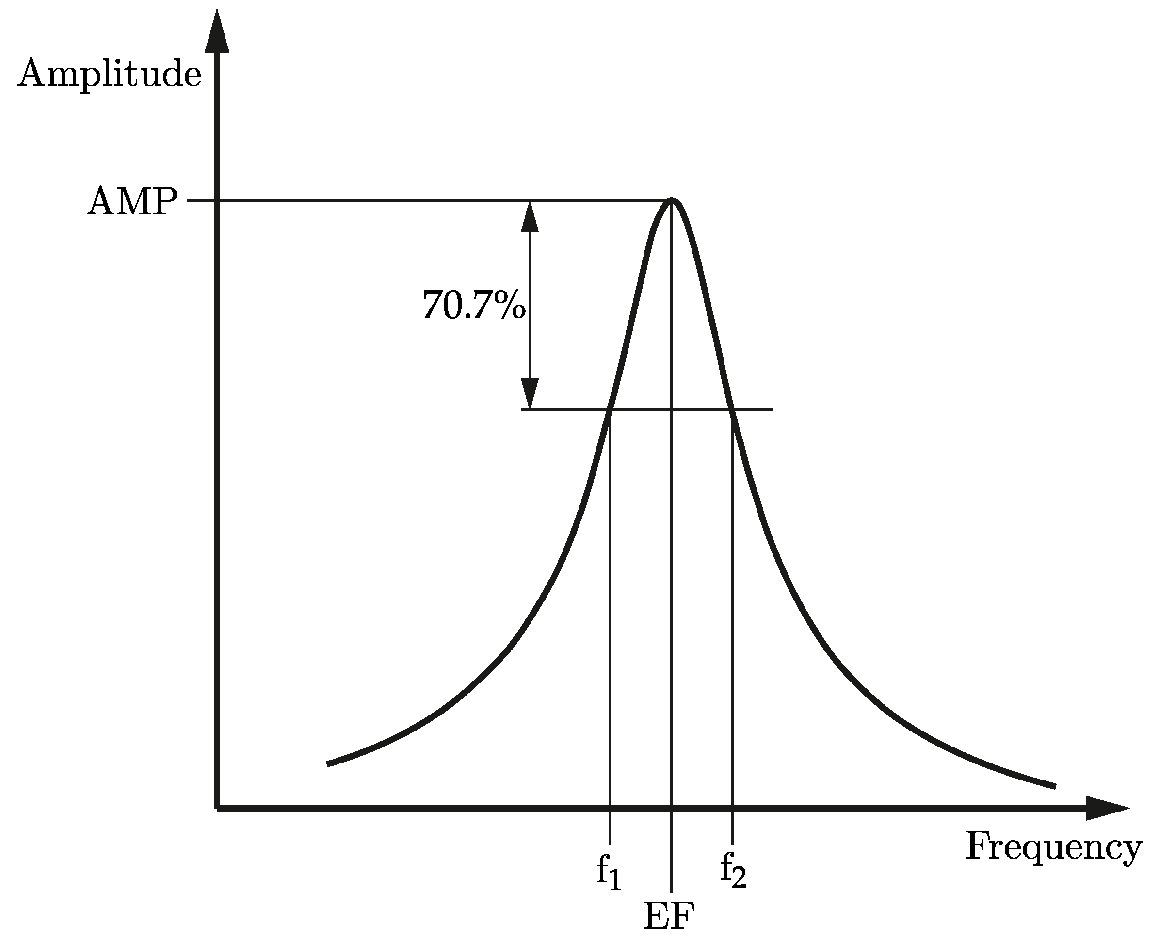
The measured FRF is used to estimate the reference values of the identification process. Peaks in the FRF curve are determined, where the eigenfrequency (EF), the amplitude at the eigenfrequency (AMP) and the normalized frequency band (NFB) are extracted as the reference values for each peak. The NFB is equivalent to the amplification factor given in [40]. This factor is estimated by the half-power method [40]. In [41], the NFB value is called the quality factor of a system and its reciprocal value is also named loss angle [1], which is an indicator for the internal friction of the material. The NFB value is given by [1,40]

$$\mathrm{NFB}=\frac{\mathrm{EF}}{f_2-f_1}.$$

(18)

The frequencies $f_1$ and $f_2$ are defined by the crossing point of the Frequency Response Function curve and a horizontal line which marks $70.7\%$ of the amplitude at the eigenfrequency. The $70.7\%$ value is often used for the description of the structural or hysteretic damping of the system and can be found in different sources, like in [40] or [1]. In Figure 1, a peak of an FRF curve including the relevant reference values is illustrated.

The presented PIP is shown for homogeneous isotropic materials. At the beginning, the complex Young’s modulus $E^{★}\left(\omega \right)$ is rewritten as [1,42]

$$E^{★}\left(\omega \right)=E^{\prime }\left(\omega \right)+\mathrm{j}{E}^{″}\left(\omega \right),$$

(19)

where $E^{\prime }\left(\omega \right)$ is the frequency depending storage Young’s modulus and $E^{″}\left(\omega \right)$ is the frequency depending loss Young’s modulus [1,42]. These two parameters are combined to $|E^{★}\left(\omega \right)|$ given by

$$|E^{★}\left(\omega \right)|=\sqrt{E^{\prime }{\left(\omega \right)}^2+E^{″}{\left(\omega \right)}^2},$$

(20)

where $|E^{★}\left(\omega \right)|$ is the frequency-dependent absolute value of the complex Young’s modulus. The parameter $\eta \left(\omega \right)$ is given as the ratio of the loss and the storage modulus [1,42]

$$\eta \left(\omega \right)=\frac{E^{″}\left(\omega \right)}{E^{\prime }\left(\omega \right)}.$$

(21)

The value $\eta \left(\omega \right)$ describes the frequency depending energy loss of the material [1,42]. This allows for rewriting the complex Young’s modulus as

$$E^{★}\left(\omega \right)=\left|E^{★}\left(\omega \right)\right|\frac{1}{\sqrt{1+\eta {\left(\omega \right)}^2}}\left(1+\mathrm{j}\eta \left(\omega \right)\right).$$

(22)

The reference values estimated from the FRF curve are values depending on a specific frequency. The complex Young’s modulus as represented in Equation (22) describes the value over a frequency range. For the following process, the unknown parameters are estimated at the specific frequencies defined by the frequency of the reference values.

2.3.2. Bisection Method

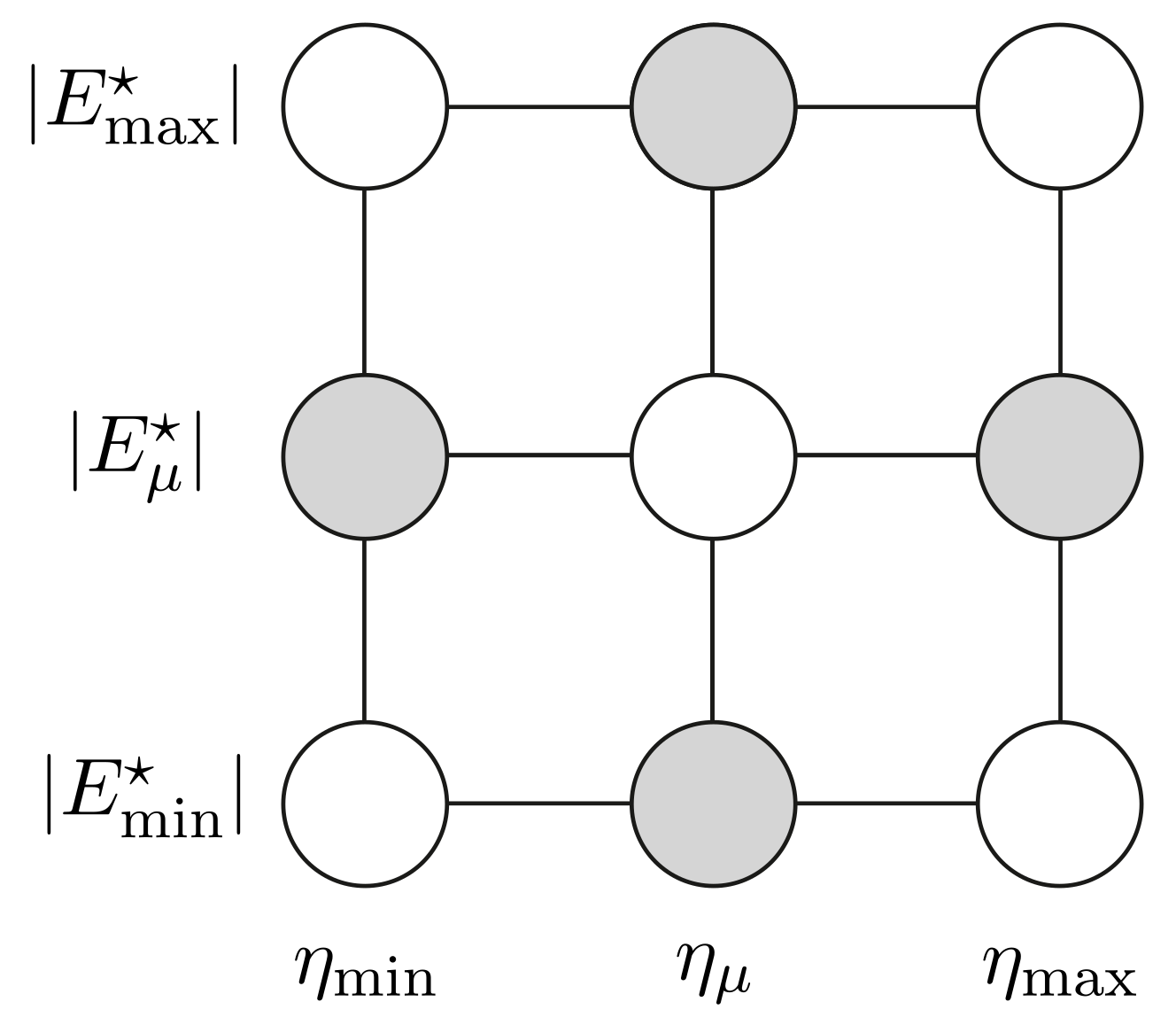
The PIP focuses first on the estimation of $|E^{★}\left(\omega \right)|$ and $\eta \left(\omega \right)$. Other parameters related to the mass or the geometry of the structure are assumed to be known or easy to measure. The first step of the process uses bisectioning on a wide range of parameter values. This method is basically used to estimate the roots of a function and uses the halving of the analyzed interval [43]. The limit values of $|E^{★}|$ and $\eta$ and the mean values are defined. This gives 9 possible parameter combinations for the bisectioning as depicted in Figure 2. Only four out of these combinations are evaluated: For the combinations marked in grey color, the eigenfrequencies and corresponding amplitudes are computed from the NAT-model described in Section 2.1 and compared to the corresponding measured values at the specific frequency.

The comparison leads to different cases to be considered:

• The combination of $|E_{\mu }^{★}|$ with both, ${\eta }_{min}$ and ${\eta }_{max}$ gives computed eigenfrequencies higher than the measured value. In this case $|E_{max}^{★}|$ is disregarded and replaced by $|E_{\mu }^{★}|$;
• Similarly, if both combinations of $|E_{\mu }^{★}|$ give a value of the computed eigenfrequency lower than the measured one, then $|E_{min}^{★}|$ is replaced by $|E_{\mu }^{★}|$;
• For the combinations of ${\eta }_{\mu }$ with both $|E_{min}^{★}|$ and $|E_{max}^{★}|$, the computed amplitudes are compared to the measured amplitude. If both computed values are higher than the measured values, then ${\eta }_{min}$ is replaced by ${\eta }_{\mu }$;
• Similarly, if both combinations are lower than the measured amplitude, ${\eta }_{max}$ is replaced by ${\eta }_{\mu }$.

The bisection method stops, when defined limit values are reached or if one calculated value is higher than the correlating reference value and one calculated value is lower than the correlating reference value. The usage of the eigenfrequency and the amplitude as reference values is adapted from [14], where the estimation of the unknown parameters is explained as the two-step identification method. In [14], the reference values EF and AMP are proved successfully for the fitting process. The third reference value is used in the bisection method as an indicator of the correct estimation of $\eta$, because [1]

$$\eta =\frac{1}{\mathrm{NFB}}.$$

(23)

The bisectioning gives rough estimates for $|E^{★}|$ and $\eta$, which are used to generate a surrogate model.

2.3.3. Surrogate Modeling

The surrogate model describes the relationship between the input parameters $|E^{★}|$ and $\eta$ on the one hand side and the output values EF, AMP and NFB on the other side. For each output parameter, an independent surrogate model is generated. Depending on the number N of peaks in the FRF curve, $3N$ surrogate models are built. In a general case, no information is given about the distribution of the input parameters, so the input parameters are chosen to be uniformly distributed. After determining the surrogate models, a large input sampling set is generated for each peak in the FRF curve depending on its limit values.

The surrogate models are evaluated for the values given by the sampling set and the corresponding output parameters are calculated. The differences between calculated and measured values are analyzed and based on this information, new limit values (the final limit values) for the input parameters $|E^{★}|$ and $\eta$ are defined. With these final limit values, new surrogate models are generated for each reference value. These final surrogate models are estimated and the corresponding final limit values for each peak in the FRF curve are determined.

2.3.4. Curve Fit

After the estimation of the final surrogate models and its corresponding limit values of $|E^{★}|$ and $\eta$, a large input sample set is generated and the surrogate models calculate the output parameters EF, AMP and NFB for each peak in the FRF curve. These calculated values per peak are compared to the reference values per peak and a finite number of fitting parameter combinations of $|E^{★}|$ and $\eta$ are estimated. These finite number of parameters are converted into the real and imaginary parts of the complex Young’s modulus $E^{★}$. This conversion has the advantage that two curves are available for the non-linear curve fit for the description of the complex Young’s modulus over the frequency range. The curve fit is executed based on the number of supporting points, which is equal to the number of peaks in the FRF curve. In Figure 3a,b the real and imaginary parts of the complex Young’s modulus for an numerical example are illustrated.

The complex Young’s modulus described in Equation (22) is describable with fractional derivative parameters based on the description of a fractional Zener model given by [35]

$$E^{★}\left(\omega \right)=\frac{a_0^E+{\left(\mathrm{j}\omega \right)}^{{\alpha }^E}{a}_1^E}{1+{\left(\mathrm{j}\omega \right)}^{{\alpha }^E}{b}_0^E}.$$

(24)

Following, the support points for the description of the real and imaginary parts of the complex Young’s modulus are used to fit the fractional derivative parameters presented in Equation (24).

2.3.5. Estimation of the Fractional Derivative Parameters

After the curve fitting process, possible fractional derivative parameter combinations are estimated. Based on the maximum error of the curve fit of the imaginary and the real part of the complex Young’s modulus, a set of appropriate fractional derivative parameter combinations is estimated. Based on these limit values of the input parameters, a large sample set of input parameters is generated and the output parameters EF, AMP and NFB are calculated from the NAT model. The values that fit the measurement are used for the generation of the surrogate models. After the generation of the surrogate models, the best fitting fractional derivative parameters are estimated.

Therefore, the range of the values of the possible fractional derivative parameters is equidistantly subdivided. Under the consideration of [35]

$$a_0^E<\frac{a_1^E}{b_0^E},$$

(25)

a large number of input sample sets is generated and the surrogate models calculate the output parameters. Following, the error of the input sample set is estimated and an error minimization is given by

$${\epsilon }_{\mathrm{REF}}=\frac{{\sum }_{i=1}^k|{\mathrm{REF}}_{i,\mathrm{calculated}}-{\mathrm{REF}}_{i,\mathrm{measured}}|}{{\mathrm{REF}}_{i,\mathrm{measured}}},$$

(26)

where REF represents the reference values EF, AMP and NFB. Based on the minimum error, the global optimum is estimated by refining the input sample space and the repeated calculation of the output parameters based on the surrogate model. Closing, the best fitting combinations for the surrogate model are estimated. These combinations are solved with the numerical model and the FRF curve of the measurement and the FRF curve based on the fractional derivative parameters estimated by the PIP are compared.

3. Results

In this section, the PIP technique is applied to estimate the fractional derivative parameters of an unknown material. First, an example is illustrated step by step to show the efficiency and accuracy of the method. Therefore, a theoretical material is used to generate a FRF curve and following, the fractional derivative parameters are estimated. Second, the process is applied to a real structure. A beam made of aluminium is analyzed and the fractional derivative parameters are estimated. NAT is implemented in MATLAB^® 2020b and the surrogate modeling process is executed by the MATLAB^® toolbox UQLab [44].

3.1. Numerical Experiment

A numerical example is used to show the PIP in detail. The beam is made of a non-existing material described by the fractional Zener model. These reference parameters are listed in

Table 1. List of the fractional derivative parameters—reference values.

${\mathit{a}}_0^{\mathit{E}}$ in $\frac{\mathbf{N}}{{\mathbf{m}}^2}$	${\mathit{a}}_1^{\mathit{E}}$ in $\frac{{\mathbf{Ns}}^{\mathit{\alpha }}}{{\mathbf{m}}^2}$	${\mathit{b}}_0^{\mathit{E}}$ in ${\mathbf{s}}^{\mathit{\alpha }}$	$\mathit{\alpha }$ in [-]
$7\times {10}^{10}$	$2.8\times {10}^8$	0.0035	0.75

.

First, the geometry of the system needs to be defined. Here, a beam with six stations and five segments is considered. The cross-sections of the beam are modeled as being circular. The diameter $d_1=d_2=d_5=0.04\mathrm{m}$ and the diameter $d_3=d_4=0.05\mathrm{m}$ describe the beam. The density of the beam is $\rho =8250\frac{\mathrm{kg}}{{\mathrm{m}}^3}$ and the Poisson number is $\nu =0.27$. The shear correction factor is calculated based on [45] for a homogeneous circular cross-section as [45]

$$k_S=\frac{6·{(1+\nu )}^2}{7+14\nu +8{\nu }^2}=0.8516,$$

(27)

where $k_S$ is the shear correction factor. The position of the stations, the additional mass moments of inertia $\mathsf{\Theta }$, and additional masses m are listed in

Table 2. List of the additional components of the numerical example.

Station	Global Coordinate x in m	Mass m in kg	Mass Moment of Inertia $\mathbf{\Theta }$ in kg m${}^2$
1	0	0.006	0
2	0.015	0.015	$9.375\times {10}^{-6}$
3	0.240	0	0
4	0.340	0.013	$8.125\times {10}^{-6}$
5	0.390	0	0
6	0.580	0.006	0

.

In Figure 4, the numerical example is illustrated.

The FRF curve is calculated in the case of the numerical example, and all the reference values are extracted. Figure 5 illustrates the FRF curve that represents a point force excitation at $x_F=0.34\mathrm{m}$ and a response at $x_R=0.015\mathrm{m}$.

As a first step, the peaks in the FRF curve (represented by dots in Figure 5), containing the reference values EF, AMP and NFB need to be determined. All four peaks are used to describe the fractional derivative parameters of the system. In

Table 3. List of the reference values of the numerical example.

Reference Point	EF in Hz	AMP in dB	NFB in −
1	361	−119.6203	22.2922
2	880	−136.1885	28.3189
3	1739	−147.0678	40.2943
4	2726	−149.9440	52.5787

, the reference values are listed. Based on the resolution of $1\mathrm{Hz}$, the frequency values needed for the estimation of the NFB value are calculated by a linear interpolation.

After the estimation of the reference values, the limit values of $|E^{★}|$ and $\eta$ of each peak in the FRF curve are determined from the bisection method presented in Section 2.3.2. The limit values of $|E^{★}|$ and $\eta$ are based on the EF and AMP reference values. The bisectioning gives rough limit values, where a difference of $10\%$ to the corresponding EF reference value and $20\%$ to the corresponding AMP reference value per peak in the FRF curve is acceptable. These tolerances are a rough limit and can be defined freely, e.g., with reference to the measurement equipment. In

Table 4. Limit values obtained from the bisection process.

Peak in the FRF	$|{\mathit{E}}_{\mathit{m}\mathit{i}\mathit{n},\mathit{B}}^{★}|$ in $\frac{\mathbf{N}}{{\mathbf{m}}^2}$	$|{\mathit{E}}_{\mathit{m}\mathit{a}\mathit{x},\mathit{B}}^{★}|$ in $\frac{\mathbf{N}}{{\mathbf{m}}^2}$	${\mathit{\eta }}_{\mathit{m}\mathit{i}\mathit{n},\mathit{B}}$ in -	${\mathit{\eta }}_{\mathit{m}\mathit{a}\mathit{x},\mathit{B}}$ in -
1	$6.3586\times {10}^{10}$	$1.0185\times {10}^{11}$	0.0183	0.2000
2	$5.7986\times {10}^{10}$	$1.2693\times {10}^{11}$	0.0183	0.2000
3	$6.3586\times {10}^{10}$	$1.0185\times {10}^{11}$	0.0183	0.2000
4	$6.3586\times {10}^{10}$	$8.2716\times {10}^{10}$	0.0183	0.0606

, the limit values of $|E_{•,B}^{★}|$ and ${\eta }_{•,B}$ depending on the peak in the FRF curve after the bisection processes are listed.

By the calculation of the reciprocal value of the NFB value, the correctness of the limits of ${\eta }_{•,B}$ is shown, referred to Equation (23). Based on this check, the correctness of the estimated values of ${\eta }_{•,B}$ is proofed and the PIP is continued.

In the next step, the surrogate models are generated with the MATLAB^® toolbox UQLab [44] based on the values listed in Table 4. The estimated limit values are used as the limit values of the uniformly distributed input parameter. Legendre Polynomials are applied to generate the multivariate orthonormal space [37]. The polynomial order p is defined and the error between the calculated results by NAT and the estimated values by the surrogate model is minimized. Based on the polynomial order p and the number of independent variables M, Equation (17) calculates the number of needed output parameters for the estimation of the surrogate model.

These generated surrogate models are evaluated and based on the quality of the model, new limit values of $|E_{•,S}^{★}|$ and ${\eta }_{•,S}$ are defined. These new and final limit values are listed in

Table 5. Limit values after the surrogate modeling analysis.

Reference Point	$|{\mathit{E}}_{\mathit{m}\mathit{i}\mathit{n},\mathit{S}}^{★}|$ in $\frac{\mathbf{N}}{{\mathbf{m}}^2}$	$|{\mathit{E}}_{\mathit{m}\mathit{a}\mathit{x},\mathit{S}}^{★}|$ in $\frac{\mathbf{N}}{{\mathbf{m}}^2}$	${\mathit{\eta }}_{\mathit{m}\mathit{i}\mathit{n},\mathit{S}}$ in -	${\mathit{\eta }}_{\mathit{m}\mathit{a}\mathit{x},\mathit{S}}$ in -
1	$7.5140\times {10}^{10}$	$7.6562\times {10}^{10}$	0.0442	0.1817
2	$7.7485\times {10}^{10}$	$8.1419\times {10}^{10}$	0.0345	0.1730
3	$7.7485\times {10}^{10}$	$7.8779\times {10}^{10}$	0.0241	0.1878
4	$7.9069\times {10}^{10}$	$7.9189\times {10}^{10}$	0.0187	0.0192

. Again, the reciprocal values of the NFB values listed in Table 3 are between in the limit values of the ${\eta }_{•,S}$ values. This shows the correct estimation of the parameters.

The final surrogate models, as described in Section 2.3.3, are used for the estimation of the possible parameter combinations for the curve fitting process. Large sample sets, based on the limit values listed in Table 5 are generated and a finite number of possible parameter combinations per peak in the FRF curve are estimated. These finite number of parameter combinations are now transformed into the real and the imaginary part of the complex Young’s modulus. Closing, the non-linear curve fit is executed for the estimation of the fractional derivative parameters described by Equation (24).

The non-linear curve fit process is executed with the MATLAB^® function lsqcurvefit. Based on these non-linear curve fits, the parameter combinations of the fractional derivative, based on the description of the complex Young’s modulus, is given. Afterwards, the normalized error at each peak in the FRF curve related to its reference value of the real part and the imaginary part is estimated.

In Figure 6a,b the errors normalized to the real and imaginary parts of the parameters estimated from the surrogate modeling are illustrated. Based on the lowest errors, the possible fractional derivative parameter values are estimated. In

Table 6. Limit values after the curve fit.

Parameter	Lower Limit	Upper Limit
$a_0^E$ in $\frac{\mathrm{N}}{{\mathrm{m}}^2}$	$6.9693\times {10}^{10}$	$7.1078\times {10}^{10}$
$a_1^E$ in $\frac{{\mathrm{Ns}}^{\alpha }}{{\mathrm{m}}^2}$	$1.2827\times {10}^8$	$3.1277\times {10}^8$
$b_0^E$ in ${\mathrm{s}}^{\alpha }$	$0.0016$	$0.0039$
${\alpha }^E$ in −	$0.7388$	$0.8281$

, the lower and upper limits of the parameters based on the error of the curve fit of the real and the imaginary part are presented.

The presented surrogate modeling process and error minimization process gives an estimation for the best fitting parameter combination.

Table 7. List of the fractional derivative parameters—example.

${\mathit{a}}_0^{\mathit{E}}$ in $\frac{\mathbf{N}}{{\mathbf{m}}^2}$	${\mathit{a}}_1^{\mathit{E}}$ in $\frac{{\mathbf{Ns}}^{\mathit{\alpha }}}{{\mathbf{m}}^2}$	${\mathit{b}}_0^{\mathit{E}}$ in ${\mathbf{s}}^{\mathit{\alpha }}$	$\mathit{\alpha }$ in [-]
$7.0036\times {10}^{10}$	$2.7655\times {10}^8$	0.0035	0.7512

lists the PIP-approximated parameters.

In Figure 7, the measured and calculated FRF curves of the numerical example are illustrated. In [6], the quality of a the parameter fit is evaluated by the comparison of the static Young’s modulus $a_0^E$. The value $a_{0,Ref}^E=7\times {10}^{10}\frac{\mathrm{N}}{{\mathrm{m}}^2}$ is used to generate this example; the value $a_{0,PIP}^E=7.0036\times {10}^{10}\frac{\mathrm{N}}{{\mathrm{m}}^2}$ is found by PIP. The relativ error is $0.051\%$. This shows the efficiency of the PIP. Additional, $\eta \left(\omega \right)$ is analyzed, to illustrate the difference between the parameters that are used for the generation of this example and the PIP-estimated values.

In Figure 8, the frequency-dependent loss value $\eta \left(\omega \right)$ of the given values of the numerical example and the fractional derivative parameters estimated by the PIP are illustrated. The dots represent the frequency points used for the PIP, which are illustrated by the peaks in the FRF illustrated in Figure 5. It is shown that with four peaks as reference, the system is described accurately.

To assess the efficient of the PIP, the computational time to compute the training set, to generate the surrogate models and the actual Parameter Identification Process is compared to a straight forward identification process without a surrogate model. All calculations are carried out on a computer operating on Windows 10, with an Intel^® Xeon^® E3-1270 processor ($4\times 3.6\mathrm{GHz}$) with $32\mathrm{GB}$ RAM. The calculations are executed with MATLAB^® 2020b.

The first step, the bisectioning process, only requires a small number of calculated reference values; therefore, the computational time is negligible compared to the other steps. The surrogate modeling process uses 8000 reference calculations to estimate the limit values of $|E^{★}|$ and $\eta$ at each reference frequency. The total computational time to calculate these reference values is approximately 6800 $\mathrm{s}$. Depending on the used polynomial order, the generation of the surrogate model takes between $0.07\mathrm{s}$ (polynomial order $p=3$) and $2.2\mathrm{s}$ (polynomial order of $p=30$). The needed parameter combinations for the description of the metamodel are calculated by Equation (17), the remaining parameter combinations are used for the quality check of the PCE. As an example, for the computation of ${10}^6$ input parameter sets (required to find a reasonable estimate of $|E^{★}|$ and $\eta$), the original NAT model requires about 236 h, while the total calculation time of the surrogate model including the training process is only 6826 $\mathrm{s}$. Therefore, the surrogate model approach is 124 times faster in this case.

3.2. Measurements

In the following, the PIP is applied for measured FRF curves obtained from a real structure.

The analyzed beam is made of aluminium. During the measurement, the test object is suspended horizontally by fishing lines with a diameter of $1\mathrm{mm}$, giving a free–free boundary condition. The test setup is illustrated in Figure 9.

The beam is excited with an electrodynamic shaker (Brüel and Kjær LDS V406, Virum, Denmark) and the response is measured with a triaxial acceleration sensor (Brüel and Kjær 84506, Virum, Denmark). The excitation force is measured with a force transducer (Brüel and Kjær 8230-001, Virum, Denmark), where a stinger is mounted between the shaker and the force sensor. The sensors are installed on the test object with a thin layer of wax on the surface. Both sensors are in the same horizontal plane. The excitation signal is sinusoidal and the system is in steady state condition when the response is measured. The duration of the measurement is one second; the resolution of the measurement is 1 $\mathrm{Hz}$. First, the time signals are recorded. Then, a FFT is obtained from the measured data and the dynamic response of the test object is estimated. Finally the Frequency Response Function signal is transformed into $\mathrm{dB}$ by the transformation of the logarithmic function.

In Figure 9, the multi-stepped beam made of aluminium $\begin{array}{|c|}\hline a\\ \hline\end{array}$ is illustrated. The force excitation is applied at the global position $x_F=340\mathrm{mm}$, in which the force is measured by a force transducer $\begin{array}{|c|}\hline b\\ \hline\end{array}$. This sensor is connected with a stinger $\begin{array}{|c|}\hline c\\ \hline\end{array}$ to a electrodynamic shaker $\begin{array}{|c|}\hline d\\ \hline\end{array}$. The response is measured at the global position $x_R=565\mathrm{mm}$ by a triaxial acceleration sensor $\begin{array}{|c|}\hline e\\ \hline\end{array}$. The support, realized by fishing lines $\begin{array}{|c|}\hline f\\ \hline\end{array}$, represents the free–free boundary condition. Screws $\begin{array}{|c|}\hline g\\ \hline\end{array}$ are used to fix the fishing lines at the beam. In Figure 10, the geometry of test object, including the position of the lumped masses and mass moments of inertia, is presented.

The stepped beam is subdivided into five segments, in which the cross-section is described by a circular and defined by diameters $d_1=d_4=d_5=0.04\mathrm{m}$ and $d_2=d_3=0.05\mathrm{m}$. The density is calculated based on the measured mass and the calculated volume of the beam as is given by $\rho =2798\frac{\mathrm{kg}}{{\mathrm{m}}^3}$. The Poisson ratio is based on a literature value of $\nu =0.34$ [46].

Equation (27) gives the shear correction factor based on the Poisson ratio, which is given by $k_S=0.8493$.

Table 8. List of the additional components of the test object.

Station	Global Coordinate x in m	Mass m in kg	Mass Moment of Inertia $\mathbf{\Theta }$ in kg m${}^2$
1	0	0.006	0
2	0.240	0	0
3	0.340	0.013	$8.125\times {10}^{-6}$
4	0.390	0	0
5	0.565	0.015	$6\times {10}^{-6}$
6	0.580	0.006	0

lists the position of the stations, the lumped masses and the mass moment of inertia of the system.

The additional masses and mass moments of inertia represent the acceleration sensor (station 5) and the force transducer (station 3) of the system, in which the lumped mass (station 1 and station 6) represent the mass of the screw.

The measured FRF curves are illustrated in Figure 11. Four curves are measured, while the test configuration is identical. The modification between the measurements is based on the variation of the force amplifier to analyze any modifications. It is shown that the measurement values are nearly equal. The anti-resonance at around $1000\mathrm{Hz}$ illustrates the different amplifier levels of the measurements.

The reference values of the measurement define the limit values of the PIP. Based on four different measurements, a range of the reference values per peak in the FRF curve is given. The limit values are listed in

Table 9. List of the reference values of the measurement.

Reference Point	${\mathbf{EF}}_{\mathbf{low}}$ in $\mathbf{Hz}$	${\mathbf{EF}}_{\mathbf{high}}$ in $\mathbf{Hz}$	${\mathbf{AMP}}_{\mathbf{low}}$ in $\mathbf{dB}$	${\mathbf{AMP}}_{\mathbf{high}}$ in $\mathbf{dB}$	${\mathbf{NFB}}_{\mathbf{low}}$ in -	${\mathbf{NFB}}_{\mathbf{high}}$ in -
1	597	597	−91.0368	−88.0468	378.1994	641.7989
2	1434	1435	−117.4343	−115.4552	244.5392	304.2220
3	2858	2862	−136.5392	−135.0089	165.7364	180.5811

. Based on the resolution of the measured Frequency Response Function curve of $1\mathrm{Hz}$, the values that are needed for the estimation of the NFB are linearly interpolated. It is shown that the variation of the eigenfrequencies EF and the amplitude AMP is small, whereas the variation of the Normalized Frequency Band NFB is larger. This is caused by the dependency of the NFB by the AMP.

Applying the bisection part, the surrogate modeling part and the curve fitting of the PIP, the limit values for estimating the fractional derivative parameters are determined. The limit values are listed in

Table 10. Limit values after curve fit.

Parameter	Lower Limit	Upper Limit
$a_0^E$ in $\frac{\mathrm{N}}{{\mathrm{m}}^2}$	$7.1306\times {10}^{10}$	$7.2445\times {10}^{10}$
$a_1^E$ in $\frac{{\mathrm{Ns}}^{\alpha }}{{\mathrm{m}}^2}$	$5.0165\times {10}^6$	$2.8050\times {10}^8$
$b_0^E$ in ${\mathrm{s}}^{\alpha }$	$4.3973\times {10}^{-14}$	$2.0652\times {10}^{-4}$
${\alpha }^E$ in [-]	$0.1951$	$0.999$

.

Finally, the best fitting parameters are determined under the consideration of global minimization. Based on the range of the limit values, a range of fitting parameters is estimated. One possible parameter combination is listed in

Table 11. List of the fractional derivative parameters—test object.

${\mathit{a}}_0^{\mathit{E}}$ in $\frac{\mathbf{N}}{{\mathbf{m}}^2}$	${\mathit{a}}_1^{\mathit{E}}$ in $\frac{{\mathbf{Ns}}^{\mathit{\alpha }}}{{\mathbf{m}}^2}$	${\mathit{b}}_0^{\mathit{E}}$ in ${\mathbf{s}}^{\mathit{\alpha }}$	$\mathit{\alpha }$ in [-]
$7.2247\times {10}^{10}$	$7.5779\times {10}^6$	$4.8713\times {10}^{-5}$	0.5142

. Therefore, one measurement is used for global minimization.

Figure 12 illustrates the measured and the calculated FRF curves. The black lines represent the measurements, whereas the dashed red line represents the parameter fit of the system.

The quality of the modeling process is shown by the accuracy of the anti-resonance around $1000\mathrm{Hz}$. The value of $a_0^E$ is similar to the value listed in the literature [46] for the static modulus of aluminium. It is shown that the system is fitted nearly perfectly. The maximum error is $1\%$. This error is shown at the third bending frequency.

4. Conclusions

The presented method shows the efficiency of combining a one-dimensional analytical description of structures with high-order polynomial surrogate modeling. No information about the system is needed initially and the limit values are estimated fast and efficiently. Based on the NFB value, a quality check of the estimated values is executed. Using surrogate modeling of the fractional derivative parameters, an estimate of the parameters can be found which describes the whole structure over a wide frequency range.

The advantages of the presented method are as follows:

• Analytical solutions of real structures are indispensable for a minimization of the error between the mathematical description of viscoelastic behavior and the real behavior of materials.
• The Polynomial Chaos Expansion, especially the MATLAB^® toolbox UQLab [44], enables a fast and efficient implementation of surrogate modeling. The high-order polynomials are an efficient way to surrogate a large numerical calculation with a minimized error.
• Based on splitting up the complex Young’s modulus into the real part and the imaginary part, two curves are used for the parameter fit, which minimizes the number of needed peaks in the FRF curve.
• The final surrogate modeling process is used to describe the whole structure with a minimum error in the representation of the whole system and the equidistant split of the input sample rang the global minimum is found directly.

References

1. Nowick, A.S.; Berry, B.S. Anelastic Relaxation in Crystalline Solids; Academic Press: New York, NY, USA; London, UK, 1972. [Google Scholar]
2. Bert, C.W. Material damping: An introductory review of mathematic measures and experimental technique. J. Sound Vib. 1973, 29, 129–153. [Google Scholar] [CrossRef]
3. Zener, C. Elasticity and Anelasticity of Metals; Chicago University Committee on Publications in the Physical Sciences, University of Chicago Press: Chicago, IL, USA, 1948. [Google Scholar]
4. Caputo, M.; Mainardi, F. Linear Models of Dissipation in Anelastic Solids. Riv. Nuovo C 1971, 1, 161–198. [Google Scholar] [CrossRef]
5. Caputo, M. Linear models of dissipation whose Q is almost frequency independent. Ann. Geophys. 1966, 19, 383–393. [Google Scholar] [CrossRef]
6. Pritz, T. Analysis of four-parameter fractional derivative model of real solid materials. J. Sound Vib. 1996, 195, 103–115. [Google Scholar] [CrossRef]
7. Ren, Z.; Atalla, N.; Ghinet, S. Optimization Based Identification of the Dynamic Properties of Linearly Viscoelastic Materials Using Vibrating Beam Technique. J. Vib. Acoust. 2011, 133, 041012. [Google Scholar] [CrossRef]
8. Menard, K.P. Dynamic Mechanical Analysis—A Practical Introduction; CRC Press: Boca Raton, FL, USA, 1999. [Google Scholar]
9. VDI 3830. VDI 3830: Damping of Materials and Members, Experimental Techniques for the Determination of Damping Characteristics, Part 5; Technical Report; Verein Deutscher Ingenieure: Düsseldorf, Germany, 2005. [Google Scholar]
10. Rouleau, L.; Pirk, R.; Pluymers, B.; Desmet, W. Characterization and Modeling of the Viscoelastic Behavior of a Self-Adhesive Rubber Using Dynamic Mechanical Analysis Tests. J. Aerosp. Technol. Manag. 2015, 7, 200–208. [Google Scholar] [CrossRef] [Green Version]
11. Huayamares, S.; Grund, D.; Taha, I. Comparison between 3-point bending and torsion methods for determining the viscoelastic properties of fiber-reinforced epoxy. Polym. Test. 2020, 85, 106428. [Google Scholar] [CrossRef]
12. Pierro, E.; Carbone, G. A new technique for the characterization of viscoelastic materials: Theory, experiments and comparison with DMA. J. Sound Vib. 2021, 515, 116462. [Google Scholar] [CrossRef]
13. Weiß, M.; Lerch, R.; Rupitsch, S.J. Simulation-Based Material Characterization of Isotropic and Direction-Dependent Polymers for Use in Active Structure Assemblies. Adv. Eng. Mater. 2018, 20, 1800417. [Google Scholar] [CrossRef]
14. Kim, S.Y.; Lee, D.H. Identification of fractional-derivative-model parameters of viscoelastic materials from measured FRFs. J. Sound Vib. 2009, 324, 570–586. [Google Scholar] [CrossRef]
15. Sun, W.; Wang, Z.; Liu, R.; Yan, X. Inverse Identification of the Frequency-Dependent Mechanical Parameters of a Viscoelastic Core Layer Based on the Vibration Response. Appl. Sci. 2017, 7, 455. [Google Scholar] [CrossRef]
16. Klanner, M.; Ellermann, K. Steady-state linear harmonic vibrations of multiple-stepped Euler-Bernoulli beams under arbitrarily distributed loads carrying any number of concentrated elements. Appl. Comput. Mech. 2020, 14, 31–50. [Google Scholar] [CrossRef]
17. Wu, J.S.; Chou, H.M. A new approach for determining the natural frequencies and mode shapes of a uniform beam carrying any number of sprung masses. J. Sound Vib. 1999, 220, 451–468. [Google Scholar] [CrossRef]
18. Brigham, J.C.; Aquino, W.; Mitri, F.G.; Greenleaf, J.F.; Fatemi, M. Inverse estimation of viscoelastic material properties for solids immersed in fluids using vibroacoustic techniques. J. Appl. Phys. 2007, 101, 023509. [Google Scholar] [CrossRef]
19. Brigham, J.C.; Aquino, W. Surrogate-Model Accelerated Random Search algorithm for global optimization with applications to inverse material identification. Comput. Methods Appl. Mech. Eng. 2007, 196, 4561–4576. [Google Scholar] [CrossRef]
20. Zhang, E.; Chazot, J.D.; Antoni, J. Parametric identification of elastic modulus of polymeric material in laminated glasses. IFAC Proc. Vol. 2012, 45, 422–427. [Google Scholar] [CrossRef]
21. Zhang, E.; Chazot, J.D.; Antoni, J.; Hamdi, M. Bayesian characterization of Young’s modulus of viscoelastic materials in laminated structures. J. Sound Vib. 2013, 332, 3654–3666. [Google Scholar] [CrossRef]
22. Xie, X.; Zheng, H.; Jonckheere, S.; Pluymers, B.; Desmet, W. A parametric model order reduction technique for inverse viscoelastic material identification. Comput. Struct. 2019, 212, 188–198. [Google Scholar] [CrossRef]
23. Sun, W.; Wang, Z.; Yan, X.; Zhu, M. Inverse identification of the frequency-dependent mechanical parameters of viscoelastic materials based on the measured FRFs. Mech. Syst. Signal Process. 2018, 98, 816–833. [Google Scholar] [CrossRef]
24. Nechak, L.; Sinou, J.J. Hybrid surrogate model for the prediction of uncertain friction-induced instabilities. J. Sound Vib. 2017, 396, 122–143. [Google Scholar] [CrossRef]
25. Sepahvand, K.; Marburg, S. Spectral stochastic finite element method in vibroacoustic analysis of fiber-reinforced composites. Procedia Eng. 2017, 199, 1134–1139. [Google Scholar] [CrossRef]
26. Sepahvand, K. Stochastic finite element method for random harmonic analysis of composite plates with uncertain modal damping parameters. J. Sound Vib. 2017, 400, 1–12. [Google Scholar] [CrossRef]
27. Prem, M.S.; Klanner, M.; Ellermann, K. Efficient parameter identification using generalized Polynomial Chaos Expansion—A numerical and experimental study. In Proceedings of the ISMA2020 International Conference on Noise and Vibration Engineering and USD2020 International Conference on Uncertainty in Structural Dynamics, Leuven, Belgium, 7–9 September 2020; pp. 1833–1846. [Google Scholar]
28. Prem, M.S.; Klanner, M.; Ellermann, K. Model parameter estimation of ball bearings using generalized Polynomial Chaos Expansion. In Proceedings of the SIRM 2021—14th International Conference on Dynamics of Rotating Machines, Gdańsk, Poland, 17–19 February 2021; pp. 331–340. [Google Scholar]
29. Schöbi, R.; Sudret, B.; Wiart, J. Polynomial-Chaos-based Kriging. Int. J. Uncertain. Quantif. 2015, 5, 171–193. [Google Scholar] [CrossRef]
30. Wiener, N. The Homogeneous Chaos. Am. J. Math. 1938, 60, 897–936. [Google Scholar] [CrossRef]
31. Cameron, R.H.; Martin, W.T. The orthogonal development of non-linear functionals in series of Fourier-Hermite functionals. Ann. Math. 1947, 48, 385–392. [Google Scholar] [CrossRef]
32. Ghanem, R.G.; Spanos, P.D. Stochastic Finite Elements: A Spectral Approach; Dover Publications, Inc.: Mineola, NY, USA, 2003. [Google Scholar]
33. Xiu, D.; Karniadakis, G.E. The Wiener-Askey polynomial chaos for stochastic differential equations. SIAM J. Sci. Comput. 2002, 24, 619–644. [Google Scholar] [CrossRef]
34. Sepahvand, K.; Marburg, S.; Hardtke, H.J. Uncertainty quantification in stochastic systems using polynomial chaos expansion. Int. J. Appl. Mech. 2010, 2, 305–353. [Google Scholar] [CrossRef]
35. Klanner, M.; Prem, M.S.; Ellermann, K. Steady-State Harmonic Vibrations of Viscoelastic Timoshenko Beams with Fractional Derivative Damping Models. Appl. Mech. 2021, 2, 797–819. [Google Scholar] [CrossRef]
36. Rao, S.S. Vibration of Continuous Systems; John Wiley & Sons, Inc.: Hoboken, NJ, USA, 2007. [Google Scholar]
37. Sudret, B. Polynomial chaos expansions and stochastic finite element methods. In Risk and Reliability in Geotechnical Engineering; Phoon, K.K., Ching, J., Eds.; CRC Press: Boca Raton, FL, USA, 2014; Chapter 6; pp. 265–300. [Google Scholar]
38. Soize, C.; Ghanem, R. Physical systems with random uncertainties: Chaos representations with arbitrary probability measure. SIAM J. Sci. Comput. 2004, 26, 395–410. [Google Scholar] [CrossRef] [Green Version]
39. Marelli, S.; Lüthen, N.; Sudret, B. UQLab User Manual—Polynomial Chaos Expansions; Technical Report; Chair of Risk, Safety and Uncertainty Quantification: ETH Zurich, Switzerland, 2021; Report # UQLab-V1.4-104; Available online: https://www.uqlab.com/pce-user-manual (accessed on 20 October 2021).
40. Avitabile, P. Modal Testing: A Practitioner’s Guide; John Wiley & Sons Ltd.: Hoboken, NJ, USA, 2018. [Google Scholar]
41. Torvik, P.J. On estimating system damping from frequency response bandwidths. J. Sound Vib. 2011, 330, 6088–6097. [Google Scholar] [CrossRef]
42. Gaul, L.; Klein, P.; Kemple, S. Damping description involving fractional operators. Mech. Syst. Signal Process. 1991, 5, 81–88. [Google Scholar] [CrossRef]
43. Burden, R.L.; Faires, J.D. Numerical Analysis; Brooks/Cole: Boston, MA, USA, 2011. [Google Scholar]
44. Marelli, S.; Sudret, B. UQLab: A framework for uncertainty quantification in Matlab. In Proceedings of the 2nd International Conference on Vulnerability, Risk Analysis and Management (ICVRAM2014), Liverpool, UK, 13–16 July 2014; pp. 2554–2563. [Google Scholar]
45. Steinboeck, A.; Kugi, A.; Mang, A.H. Energy-consistent shear coefficients for beams with circular cross sections and radially inhomogeneous materials. Int. J. Solids Struct. 2013, 50, 1859–1868. [Google Scholar] [CrossRef] [Green Version]
46. Kovácik, J.; Marsavina, L.; Linul, E. Poisson’s Ratio of Closed-Cell Aluminium Foams. Materials 2018, 11, 1904. [Google Scholar] [CrossRef] [PubMed] [Green Version]
Figure 1. Schematical representation of a peak including the reference values.
Applmech 02 00056 g001
Figure 2. Schematical representation of the bisection estimated values at a specific frequency.
Applmech 02 00056 g002
Figure 3. Real and imaginary parts of the complex Young’s modulus. (a) Re[ E ( ω ) ]; (b) Im[ E ( ω ) ].
Applmech 02 00056 g003
Figure 4. Model of the numerical example.
Applmech 02 00056 g004
Figure 5. Reference FRF curve of the numerical example.
Applmech 02 00056 g005
Figure 6. Normalized errors. (a) Real part; (b) imaginary part.
Applmech 02 00056 g006
Figure 7. Comparison of the reference FRF curve and the FRF curve estimated by the PIP.
Applmech 02 00056 g007
Figure 8. Schematically representation of a peak including the reference values.
Applmech 02 00056 g008
Figure 9. Illustration of the test setup—created by author.
Applmech 02 00056 g009
Figure 10. Model of the test object.
Applmech 02 00056 g010
Figure 11. Measured FRF curves of the test object.
Applmech 02 00056 g011
Figure 12. Comparison of the measured FRF curves of test object and the FRF curve estimated by the PIP.
Applmech 02 00056 g012