1. Introduction
Theoretical models based in Space Truss Analogy (STA) has been widely used for the analysis of the behavior of reinforced concrete (RC) beams under torsion. Currently, these models constitute the basis of several design codes, such as the fib Model Code and the ACI (American Concrete Institute) Code.
Over the last four decades, there has been a high focus on STA developments. One of the most important development is the Variable Angle Truss Model (VATM) proposed in 1985 by Hsu and Mo [
1], which for the first time incorporated a softened stress (
)–strain (
) relationship for the concrete in compression in the struts. Several studies shown that the VATM predicts well the ultimate behavior of RC beams under torsion. However, neither the cracking torque nor the torsional stiffness in the cracked stage are well predicted by the VATM. This is because the model does not account for the concrete tensile strength [
1,
2]. Despite further refinements of the VATM [
3,
4,
5,
6], the model still remained valid only to predict the ultimate behavior of beams under torsion.
In addition to the ultimate limit state, codes rules also refer the need to check the behavior of the beams for low loading levels (serviceability limit states). For this reason, recent improvements of theoretical models based on STA have aimed to also provide good estimates for low loading levels. In 2009, Jeng and Hsu [
7] proposed the Softened Membrane Model for Torsion (SMMT), which constitutes an extension of the previous Softened Membrane Model (SMM) [
8]. Bernardo et al. in 2012 proposed the Modified Variable Angle Truss Model (MVATM) [
9] and, in 2015, the Generalized Softened Variable Angle Truss Model (GSVATM) [
10], both as an extension of the VATM. All these improved models incorporate the influence of tensile concrete behavior through an appropriate
relationship for concrete in tension in the perpendicular direction to the struts. For this reason, the referred models give good predictions for the full behavior of RC beams under torsion, namely the torque (
)–twist (
) curve, including the uncracked, cracked, and ultimate states.
When compared to MVATM, both SMMT and GSVATM are theoretically more consistent because they are based on one unique theory. VATM is recognized as an analytical model which provides a simple physical understanding of how a RC beam behaves under torsion. For these reasons, the GSVATM is used in this study.
In practice, torsion is usually combined with other internal forces. For this reason, theoretical models need to be extended to cover combined loadings. In a previous study, the authors successfully extended the GSVATM for prestressed concrete beams (with longitudinal and uniform prestress) under torsion [
11]. Until now, the GSVATM was mainly validated for beams under pure torsion. In this article, the GSVATM is extended to the case of torsion combined with a uniform axial stress state due to an axial centered force. Since torsion is considered to be the primary effect, only cases with low to moderate axial stress states (both compression and tension) are considered. Although this particular loading case is not widely used in current practice, its study will allow one to preliminarily calibrate and check the GSVATM for this combined loading before it can be extended to more complex types. Moreover, this study will also allow researchers to analyze and understand the influence of low to moderate axial stress states on the behavior of RC beams under torsion.
In this article, these changes in the GSVATM formulation and calculation procedure are presented. Since no experimental data leading with RC beams under torsion combined with constant axial force were found in the literature, a reference RC beam was used for computation by using GSVATM, the theoretical response under torsion combined with several levels of external axial centered forces (both compression and tension). To validate the theoretical results, they are compared with the numerical results from nonlinear finite element method (FEM) applied to the same reference beam and loading cases. For convenience, the used reference beam is beam A2, tested under pure torsion by Bernardo and Lopes [
12] and also previously modeled under pure torsion with the non-linear FEM by Ferreira in 2016 [
13]. The adopted methodology to validate the results from GSVAM can be justified because, in recent years, FEM software packages have proven to be reliable for nonlinear incremental analysis. The comparative analysis was performed based on the theoretical and numerical
curves, namely the shape and some of the key points.
2. Original GSVATM Formulation and Calculation Procedure
As also presented in the previous article from the authors [
11], for the sake of this article and also to help the reader to better understand
Section 3,
Table 1 illustrates the models and summarizes the equations from GSVATM for RC beams under torsion. More details about the original GSAVTM can be found in [
10].
As presented in
Table 1, a plain truss analogy is assumed to model a RC thin beam element under shear force
(which induces a shear flow
in the cross section), GSVATM incorporates an additional tensile force
(concrete tie) perpendicular to the concrete strut with compressive force
, and angle
to the longitudinal axis. The resultant force
, with an angle
(Formula (2)) to
and an angle
(Formula (3)) to the longitudinal axis, is computed from Formula (1). The forces
(Formula (4)) and
(Formula (5)) are the resultants of the compressive and tensile stress fields in concrete (
and
, respectively), with
being the distance between centers of the longitudinal bars and
the width of the cross section, which is assumed to be equal to the width of the compressive and tensile concrete stress field (concrete strut and concrete tie, respectively).
The outer shell of a box beam element under a torque
can be modeled as the union of four thin beam elements under shear as previously presented (see
Table 1). Bredt′s thin tube theory is used to relate
with the circulatory shear flow
. From the space truss analogy, three equilibrium formulas are derived to compute
(Formula (6)), the effective thickness
of the concrete strut and tie (Formula (7), which is multiplied by (-1) if
), and the angle
of the concrete struts (Formula (8)). In Formulas (6)–(8),
is the area enclosed by the center line of the shear flow (which is assumed to coincide with the center line of the walls:
, with
and
being the minor and major outer dimension of the rectangular section),
is the perimeter of the center line of the shear flow (
),
is the total area of longitudinal steel,
is the area of one bar of the transverse steel,
is the longitudinal spacing of the transverse reinforcement, and
and
are the stresses in the longitudinal and transverse reinforcement, respectively.
A set of three compatibility formulas (see
Table 1) are also derived to compute the strain in the transverse reinforcement
(Formula (9)) and longitudinal reinforcement
(Formula (10)), as well as the twist per unit length of the beam
(Formula (11)). A useful invariant equation is also derived from Mohr´s circle for strains (Formula (12)) in order to relate the strains. In Formulas (9) to (12),
is the maximum compressive strain at the surface of the strut,
and
are the average strains in the concrete tie and strut, respectively.
A smeared and softened
relationship must be adopted to model the nonlinear behavior of the diagonal concrete struts. Smeared and stiffened
relationships must also be adopted to model the nonlinear behavior of the diagonal concrete ties and steel bars. The following
relationships were used for GSVATM [
10,
11]:
For concrete in compression:
relationship proposed by Belarbi and Hsu in 1994 [
14] (Formulas (13) and (14), see
Table 2) with softening factors (
, both for the peak stress and corresponding strain) proposed by Zhang and Hsu in 1998 [
15] (Formulas (15)–(18), see
Table 2);
For concrete in tension:
relationship proposed by Belarbi and Hsu in 1994 [
14] and modified by other authors for RC plain [
7] and hollow [
16] beams under torsion (Formulas (19)–(23), see
Table 2);
For steel bars in tension:
relationship proposed by Belarbi and Hsu in 1994 [
14] (Formulas (30)–(32), see
Table 2).
In
Table 2,
is the uniaxial concrete compressive strength,
is the strain corresponding to
,
is the longitudinal reinforcement ratio (
, with
),
is the transverse reinforcement ratio (
, with
),
and
are the yielding stress for the longitudinal and transverse reinforcement, respectively,
is the Young´s modulus for concrete,
is the concrete cracking stress and
is the strain corresponding to
,
and
are the stress and strain in the steel bars, respectively,
is the Young´s Modulus for steel,
is the yielding stress of steel bars, and
is the reinforcement ratio.
Due to the bending of the walls, a strain gradient exists along the wall´s thickness. For this reason, the stresses in the diagonal concrete strut
and in the diagonal concrete tie
are defined as the average stress of non-uniform stress diagrams (Formulas (24) and (27), see
Table 2). Parameters
(Formulas (25) and (26)) and
(Formulas (28) and (29)) are the average compressive and tensile stresses, respectively, and they can be obtained by integrating Formulas (13) and (14) and Formulas (19) and (20).
The solution procedure to compute the
curve from GSVATM is based on a trial-and-error technique, because unknowns and interdependent variables exist when calculations are initiated. The calculations are initiated for each input value of the strain at the outer fiber of the concrete strut (
). Details of the solution algorithm for the GSVATM can be found in [
10].
3. GSVATM for RC Beams under Torsion Combined with Axial Force
In this section, the GSVATM is extended to include the interaction of torque () with an axial external force (). For this latter, both tensile and compression forces are considered. It is assumed that is positive for axial tensile forces and negative for axial compressive forces. The case with a positive is chosen to present the changes in GSVATM.
It is assumed that
simply imposes an additional and axial uniform stress state in the RC beam, in addition to the one imposed by
. Then,
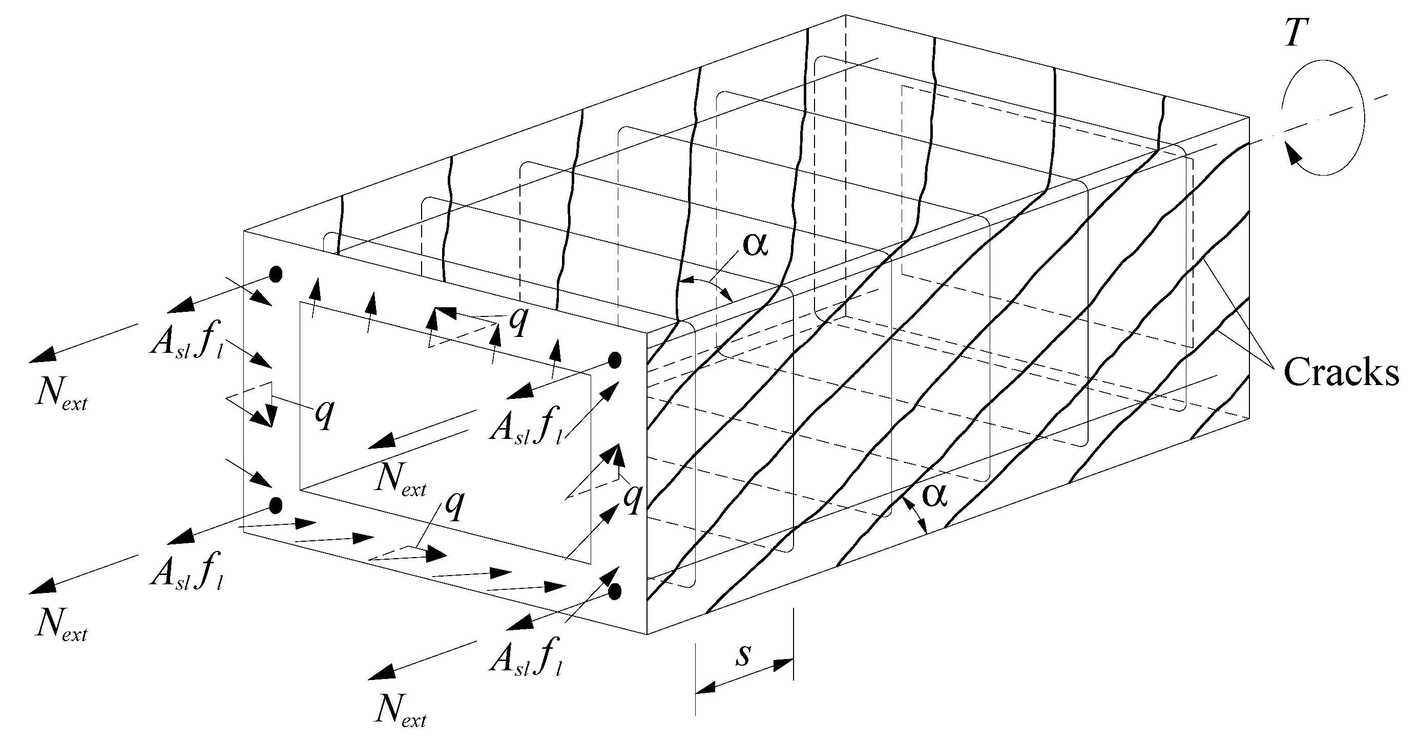
must be accounted for the longitudinal equilibrium for the RC box beam under torsion (
Figure 1). It is assumed that
is carried by the longitudinal reinforcement, so
must be simply added to the tensile force in the longitudinal reinforcement (
) due to torsion in the longitudinal equilibrium equation from GSVATM [
10]. This assumption was also assumed by Hsu to extend the VATM for RC beams under torsion combined with an axial force [
17]. The new longitudinal equilibrium equation is as follows (which needs to be multiplied by (−1) if
):
From Equation (1), and among the set of equilibrium equations from GSVATM (
Table 1), only Formula (7) needs to be modified to compute the effective thickness
tc for the concrete struts and ties. The new equation is Equation (2), which also needs to be multiplied by (-1) if
.
Also, the equation to compute the angle
of the concrete struts (Formula (8)) needs to be modified to include the additional stress state. Formula (6) from
Table 1 remains unchanged.
In addition to the axial stress state,
also imposes an additional and initial strain state in the longitudinal direction. The initial strain in the longitudinal reinforcement due to
and
can be computed from Equation (4), where
is the area bounded by the outer perimeter of the cross section and
is the hollow area of the box section (
for plain sections). This initial strain must be added to the strain in the longitudinal reinforcement due to torsion
, which is computed from Formula (10) (
Table 1). Thus, for RC beams under torsion combined with an axial force, the effective strain in the longitudinal reinforcement,
is the sum of the two previous strains (Equation (5)).
The remaining compatibility equations from
Table 1 remain unchanged. Invariant Formula (12) in
Table 1 also remains valid because the contribution of
is incorporated through
.
It should also be noted that, for RC beams under torsion combined with an axial compressive force, a pre-decompression stage, similar to the one for beams under torsion with longitudinal prestress [
11], also exists. At this stage, the shape of the curve
is perfectly linear because the stress levels are still very low. Thus, it is assumed that the modified GSVATM will only start the calculations at the end of the decompression stage. This simplification allows for the simplification of the calculation procedure, because it avoids modeling and computing the evolution of the initial compressive stresses in the truss elements, which tends to be in tension due to torsion (concrete tie and longitudinal bars). This procedure was also adopted by Hsu and Mo in 1985 [
3] and Bernardo et al. in 2018 [
11] when they extended the VATM and the GSVATM for prestressed concrete (PC) beams under torsion, respectively.
To compute the stresses from the strains, the same smeared
relationships used in the original GSVATM to model the nonlinear behavior of the materials are also used here (
Table 2).
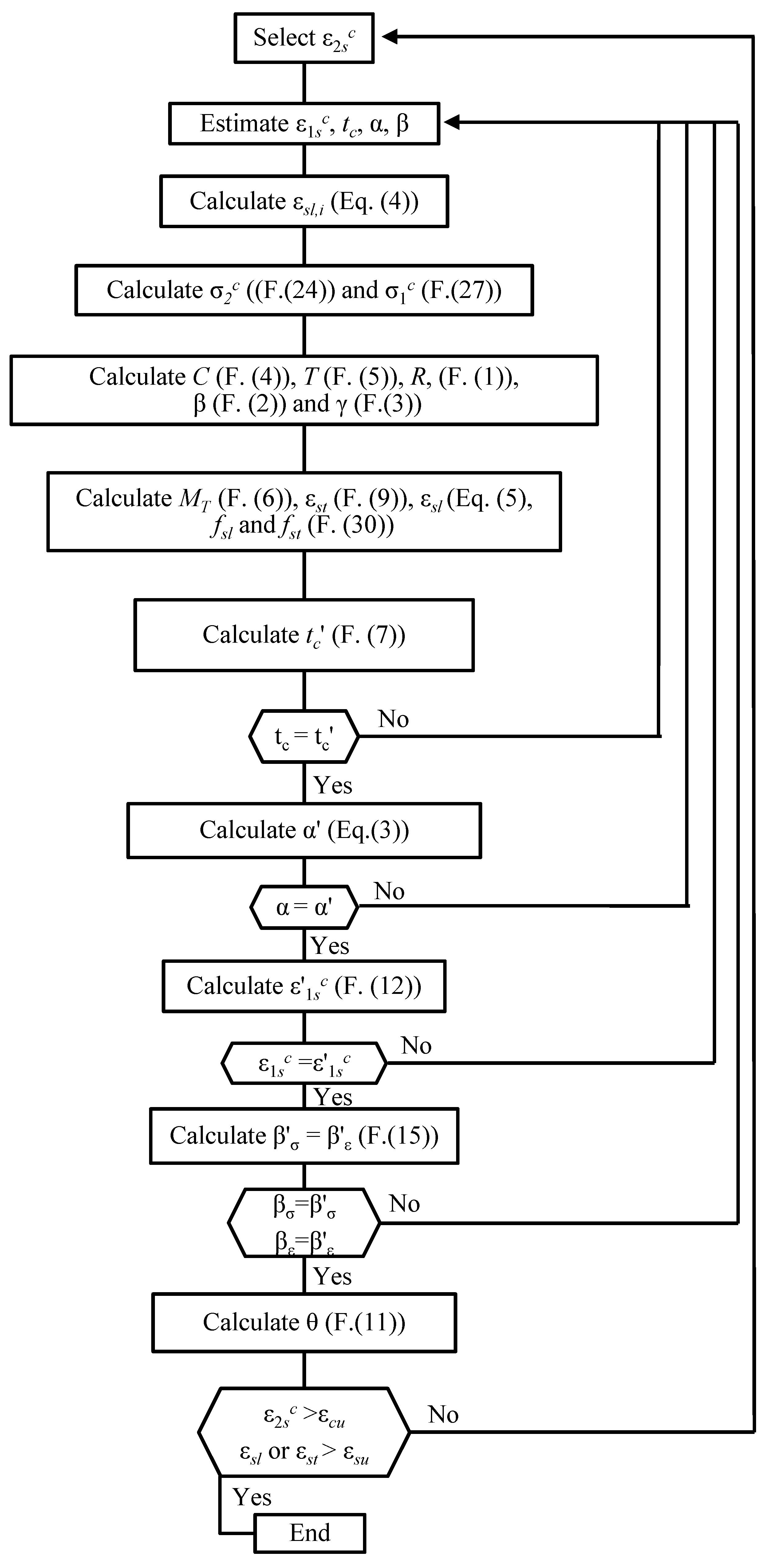
For RC beams under torsion combined with axial force, the calculation procedure to compute the theoretical
curve is similar to the one from the original GSVATM [
10]. The calculation procedure starts with an initial assumed value for the strain at the outer fiber of the concrete strut
and also with initial estimates for some of the other variables. Then, a trial-and-error methodology is used to converge to the solution point, which corresponds to the first point of the
curve with coordinates (
;
). Hereafter,
is incremented and a new iterative cycle is started until the next solution point is obtained. The calculation procedure ends when the theoretical failure of the RC beam is reached. It is assumed that the theoretical failure occurs when the strain in the outer fiber of the concrete strut,
, reaches the ultimate conventional value
, or when the strain in the longitudinal,
, and/or transverse,
, reinforcement reaches the ultimate conventional value
. In this study, the conventional ultimate strains for the materials defined by Eurocode 2 [
18] has been considered.
Figure 2 presents the flowchart for the iterative calculation algorithm used in this study to compute the theoretical
curve of RC beams under torsion combined with axial force. For the computational implementation of GSVATM, the Delphi programming language has been used.
4. Comparative Analysis with Numerical Results
In order to validate the extended GSVATM for RC beams under torsion combined with axial force, this section presents a comparative analysis between some theoretical results from GSVATM with the numerical ones using nonlinear finite element analysis (FEA) by using Abaqus software [
19]. For this, and as referred to in
Section 1, the RC hollow beam A2 (beam A-47.3-0.76 in the original notation) tested under torsion by Bernardo and Lopes in 2009 [
12] is used as reference beam. Beam A2 has the following relevant characteristics: a hollow squared cross section (0.60 × 0.60 m) with wall thickness 10.7 cm, symmetrical longitudinal reinforcement with 4φ12 mm (one rebar in each corner) + 12φ10 mm (3 rebars in each wall), transverse reinforcement φ8 mm with longitudinal spacing 8 cm, balanced longitudinal and transverse reinforcement ratios (
and
), concrete cover 2.9 cm, average compressive concrete strength
, average steel yielding strength
, and ductile failure mode.
4.1. FEA Modelling
Beam A2 was modeled with continuous solid hexahedral finite elements with linear geometry C3D8R [
19], with eight nodes and with three degrees of freedom per node. The nonlinear behavior of the concrete was considered through the Concrete Damaged Plasticity (CDP) model, which models the concrete behavior both for compression and tension. CDP uses the concept of isotropic damaged elasticity in combination with isotropic tensile and compressive plasticity to model the inelastic behavior of concrete. For the failure criteria, CDP assumes two mechanisms: the cracking of concrete in tension and the crushing of concrete in compression. Tensile concrete damage is quantified by dissipation of the fracture energy
required to create microcracks, which is computed as the area under the
curve for concrete in tension. The cracks propagation is modeled based on a mechanism of continuous damage, called stiffness degradation.
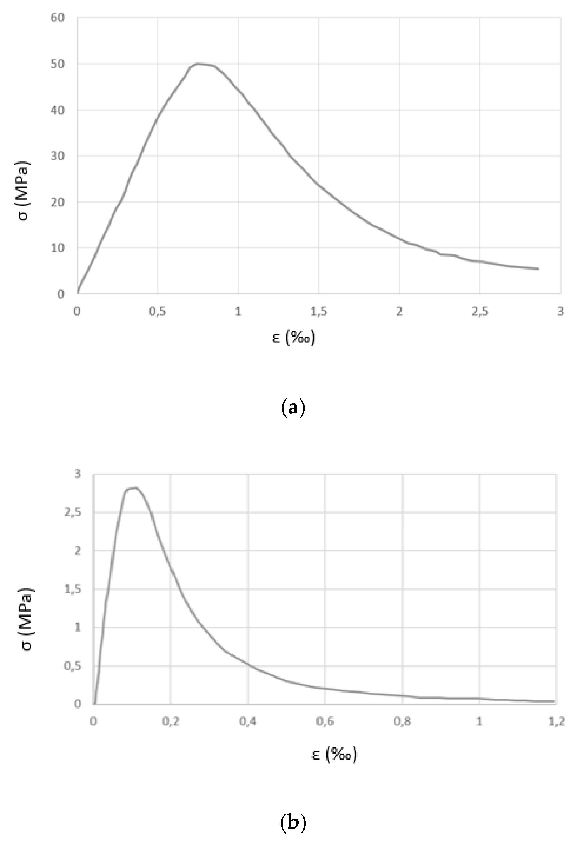
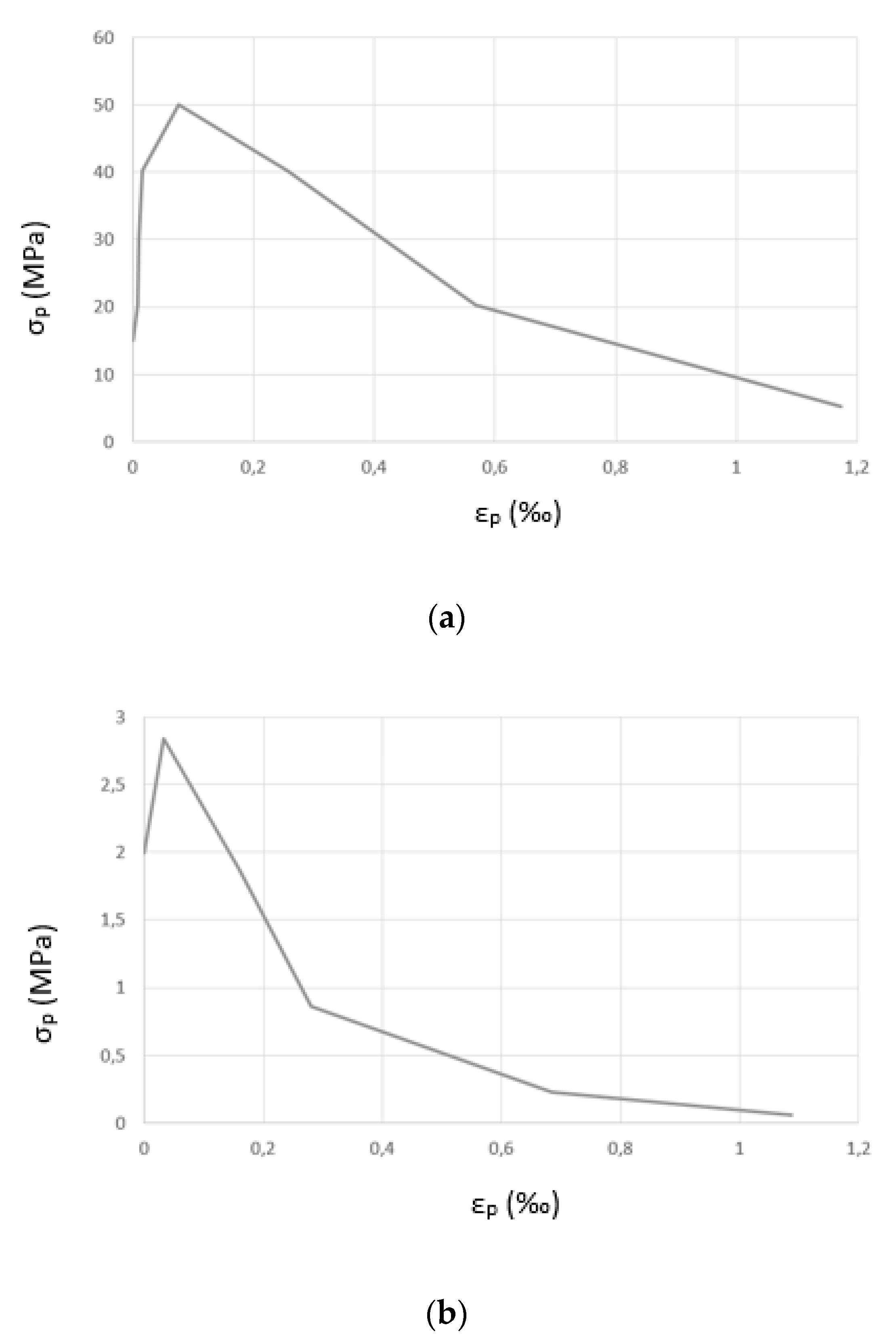
For this study, the concrete of Beam A2 was characterized using the same criteria used by Jankowiak and Łodygowski in 2005 [
20] to define the parameters for the CDP model for a very similar concrete with compressive strength equal to 50 MPa.
Figure 3 and
Figure 4 present the adopted
and plastic stress (
)–plastic strain (
) relationships for concrete in compression and tension.
The following values for concrete parameters incorporated into the CDP [
18] were considered: Young´s modulus
, Poisson´s coefficient
, dilatation angle
, eccentricity
, ratio between the initial equibiaxial compressive yield stress to the initial uniaxial compressive yield stress
, ratio between the second stress invariant to the tensile meridian and the compressive meridian
(
), and viscoplastic regularization parameter
. Most of these values were calibrated by using recommendations from the literature [
21]. Details about these parameters can be found in Abaqus manuals.
Longitudinal and transverse rebars were modeled with T3D2 FE bar type elements [
19], which is a straight bar element with 3D linear geometry and two nodes. Each node has three degrees of freedom, which make this element compatible with the three-dimensional C3D8R FE used to model the concrete.
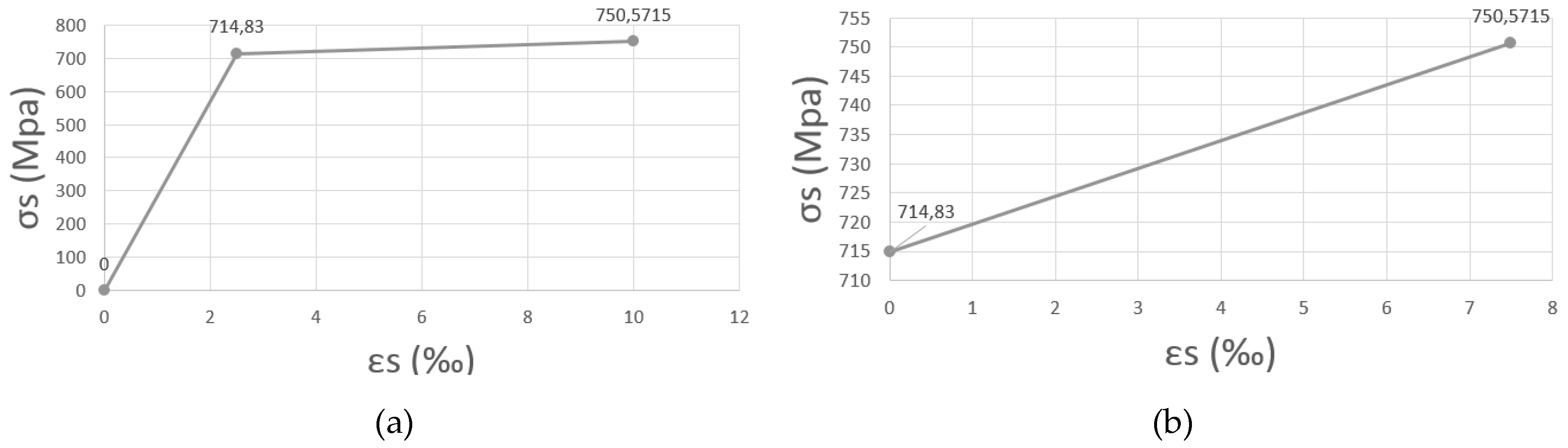
To describe the elastic-plastic behavior of the reinforcement in tension, the uniaxial bilinear
constitutive relationship from Eurocode 2 (EC2) [
18] was adopted. The limit for the elastic strain (0.0025) was calculated based on the ratio of the yielding strength to the Young’s modulus (200 GPa). The ultimate limit for the strain was considered to be 0.010. Parameter
in Abaqus, which is defined as the ratio between the tensile strength to the yielding strength, was assumed to be 1.05 (corresponding to a ductility Class A steel according to EC2 [
18]). The Poisson´s ratio was considered equal to
. For the reinforcement, a linear and elastic behavior was assumed up to the elastic limit strain, followed by a plastic behavior until failure. To model the plastic behavior, the Classic Metal Plastic (CMP) model incorporated into Abaqus [
19] was adopted. In this model, after the yielding stress is reached, the standard definitions of metal plasticity govern the properties of the bar elements. This model is basically defined by the plastic
relationship, where the initial stress value corresponds to the maximum stress for which the plastic strain is zero, which is equal to the tensile stress limit value. CMP only requires the
relationship for the plastic zone, that is,
.
Figure 5 shows the adopted
curves for rebar φ10 mm, as example.
Nodal restrictions were adopted in the top cross sections of the beam model, namely to simulate the full restrained twist condition in one top cross section and the equivalent action to the external torque (imposed twists) in the other one. In order to avoid premature failure and convergence problems at the ends of the beam model due to stress concentrations, the endings of the beam (with 25 cm thickness in the longitudinal direction) were modeled as if they were made with purely elastic concrete without strength limit. To model these zones, the same C3D8R element was used.
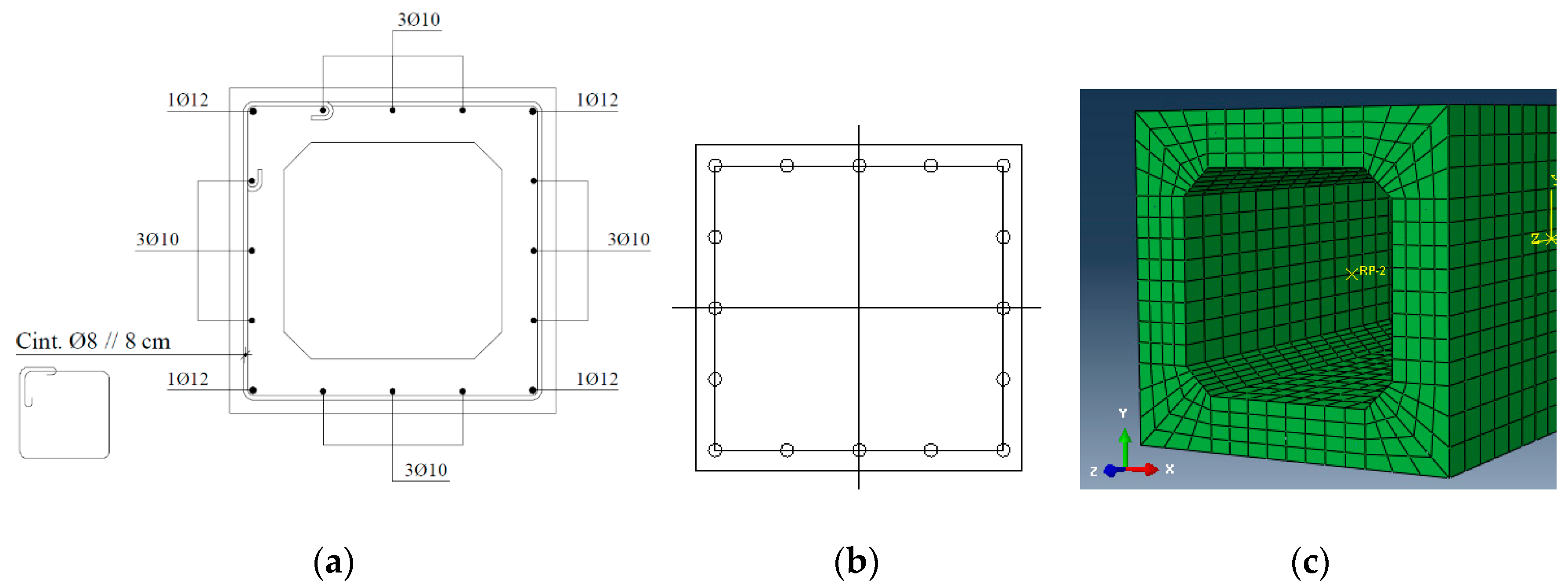
To simplify the modeling of the beam’s reinforcement (
Figure 6a), it was considered that the axes of both longitudinal and transverse rebars lie in the same plane (
Figure 6b).
The interconnection between steel bar and concrete finite elements (FE) was simulated using the Embedded Regions technique incorporated into Abaqus [
19]. In such a technique, the translational degrees of freedom of the embedded element nodes are interpolated from the degrees of freedom of the host element nodes by using geometrical relationships between the embedded and host elements, while the rotational degrees of freedom are kept free. To minimize convergence problems, the nodes of the bar elements are located inside the host elements (the nodes of the embedded and host elements have different coordinates in the longitudinal direction) [
21].
In order to obtain good accuracy, the FEM mesh must be as refined as possible and also must follow the geometry of the cross section with a uniform pattern [
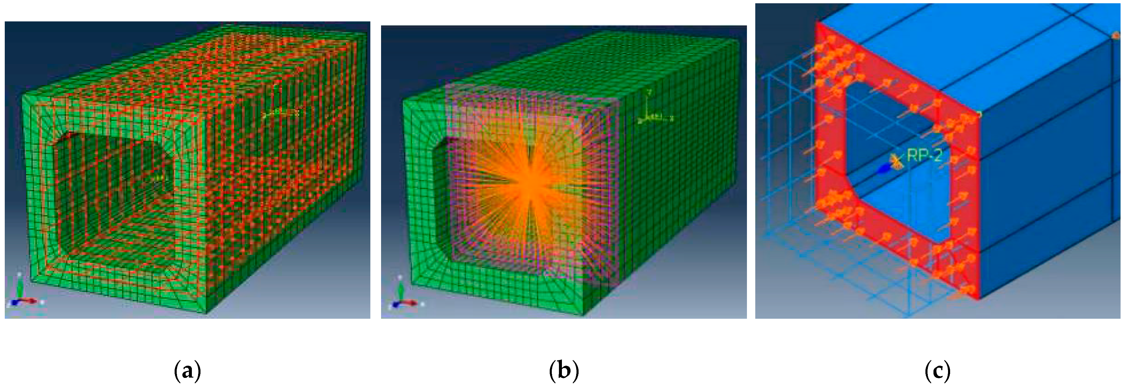
22]. The mesh creation was performed independently for each component (concrete and reinforcement). After several simulations,
Figure 6c shows the adopted FEM mesh. The final size and the geometry of the FEM mesh were chosen as function of the wall´s thickness. After some simulations and to reduce the calculation time, it was possible to reduce the length of the FE model to 1.5 m (the real length of beam A2 is almost 6.0 m), see
Figure 7.
Figure 7 shows the model of the reinforcement embedded in the concrete (
Figure 7a), the location of RP1 in one of the top beam (
Figure 7b), and the axial stress state acting on one top of the model (
Figure 7c).
To materialize both the supports and load application points, coupling restrictions were introduced in the model with respect to two created reference points (RP1 and RP2). In RP1, the transverse translations and the twist were blocked. The longitudinal translations were not impeded in order to allow the warping of the cross sections. However, to minimize convergence problems, the longitudinal translation was blocked at one single point along the model. In RP2, an upper limit of 0.07 rad was imposed for the imposed twist. This value was defined based on the maximum value experimentally recorded for beam A2 [
12].
4.2. Numerical Results and Comparative Analysis with GSVATM
By using the numerical model presented in the previous section, the behavior of reference beam A2 was simulated under increasing torques combined with different levels of constant axial forces, both compressive and tensile. The aim is to validate the extended GSVATM, as presented in
Section 3, based on a comparative analysis between the predictions from GSVATM for beam A2 and the numerical results from FEM.
The chosen uniform axial stresses induced by the axial forces, both compressive
and tensile
stresses, are limited to low to moderate levels. This is to ensure that torsion remains the primary internal force and that the global behavior of the beam is mainly governed by torsion, including the failure mode. The chosen criterion is that the maximum level for the stresses induced by the axial forces, when acting alone (without torsion), do not lead to concrete behaving nonlinearly. For this, EC2 [
18] was used to establish the limit values of the axial stress states induced by the axial force. According to EC2, it can be assumed that concrete in compression shows a linear behavior up to 45% of its characteristic compressive strength
, thus the limit for the compressive stress was assumed to be
, where
is the average compressive strength (same as
). The rules from EC2 were used to compute
from
. To limit the tensile stress, the average tensile strength of concrete
was considered as the maximum allowed value, in order to avoid cracking due to the tensile axial force. Thus, from EC2, the limit for the tensile stress is
.
Based on the above, five levels of compressive stress
, and four levels of tensile stress
, were considered to simulate beam A2 under torsion.
Table 3 presents the considered levels of axial stresses for beam A2, as well as their corresponding axial forces
.
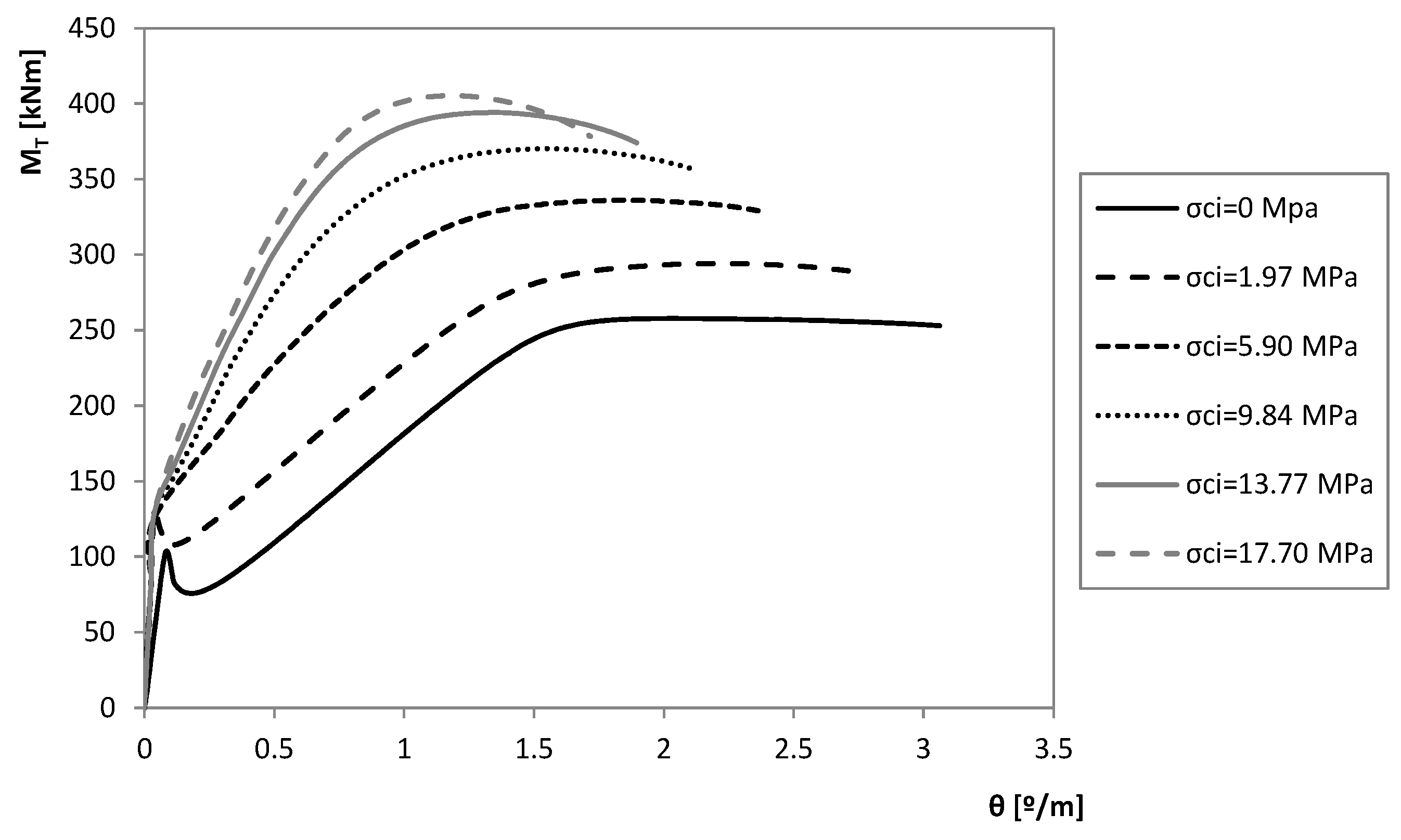
Figure 8 presents the theoretical
curves computed from GSVATM for beam A2 under torsion combined with the different compressive axial stress states
, presented in
Table 3. From
Figure 8, it can be observed that both the resistant torque and the torsional stiffness in the cracked state increase as
increases. The increase of the stiffness leads to a decrease in the twist corresponding to the resistant torque. These tendencies agree with the results from previous studies on RC beams with compressive axial stress states, namely from Bernardo et al. in 2015 [
23] for RC beams in torsion that are axially restrained and Lopes et al. in 2017 [
24] for RC beams in bending that are also axially restrained. From their studies, the authors concluded that the existence of a moderate axial compression state due to a confinement effect is favorable for both the resistance and stiffness of the RC beam, since it reduces the tensile state imposed by the torque or bending moment.
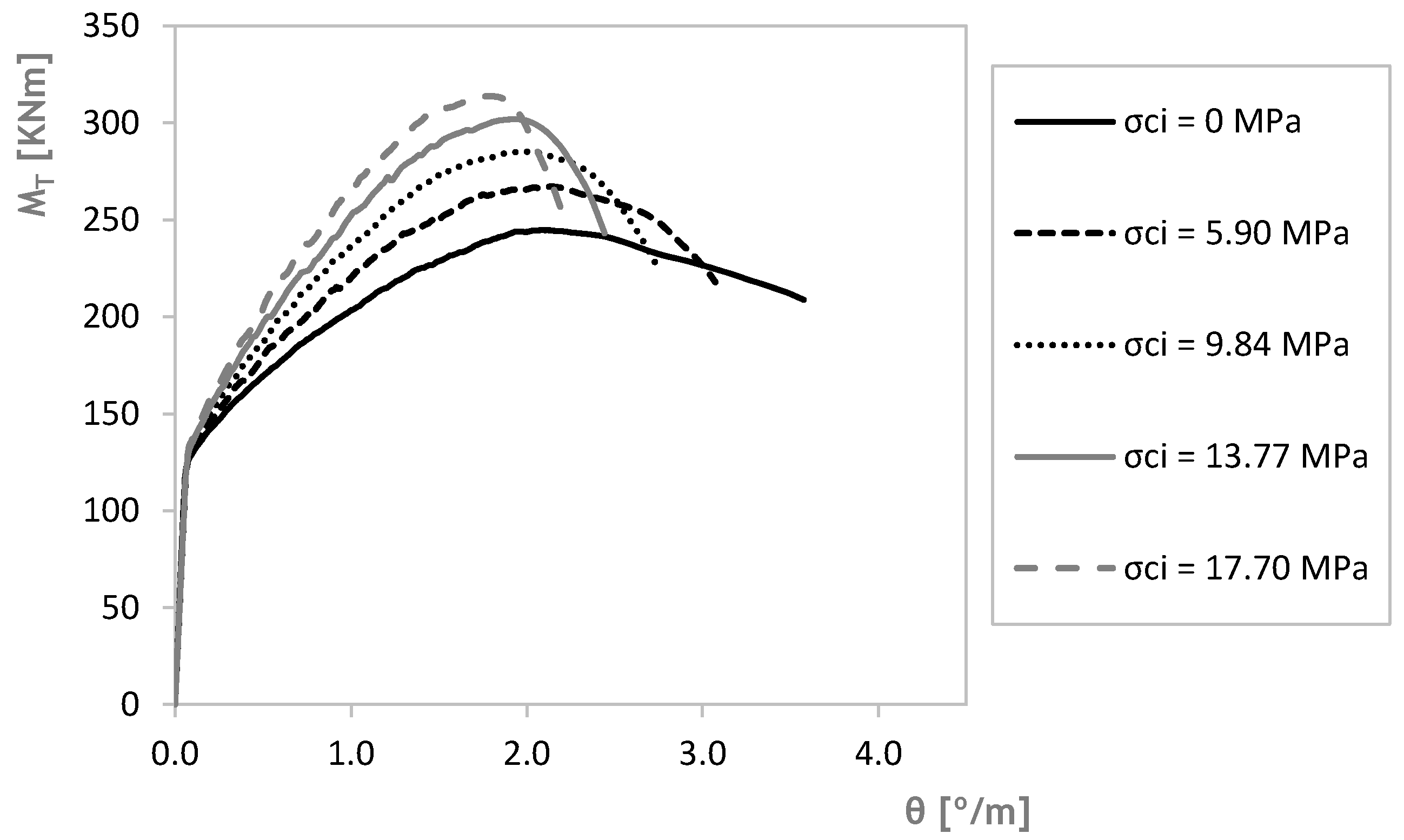
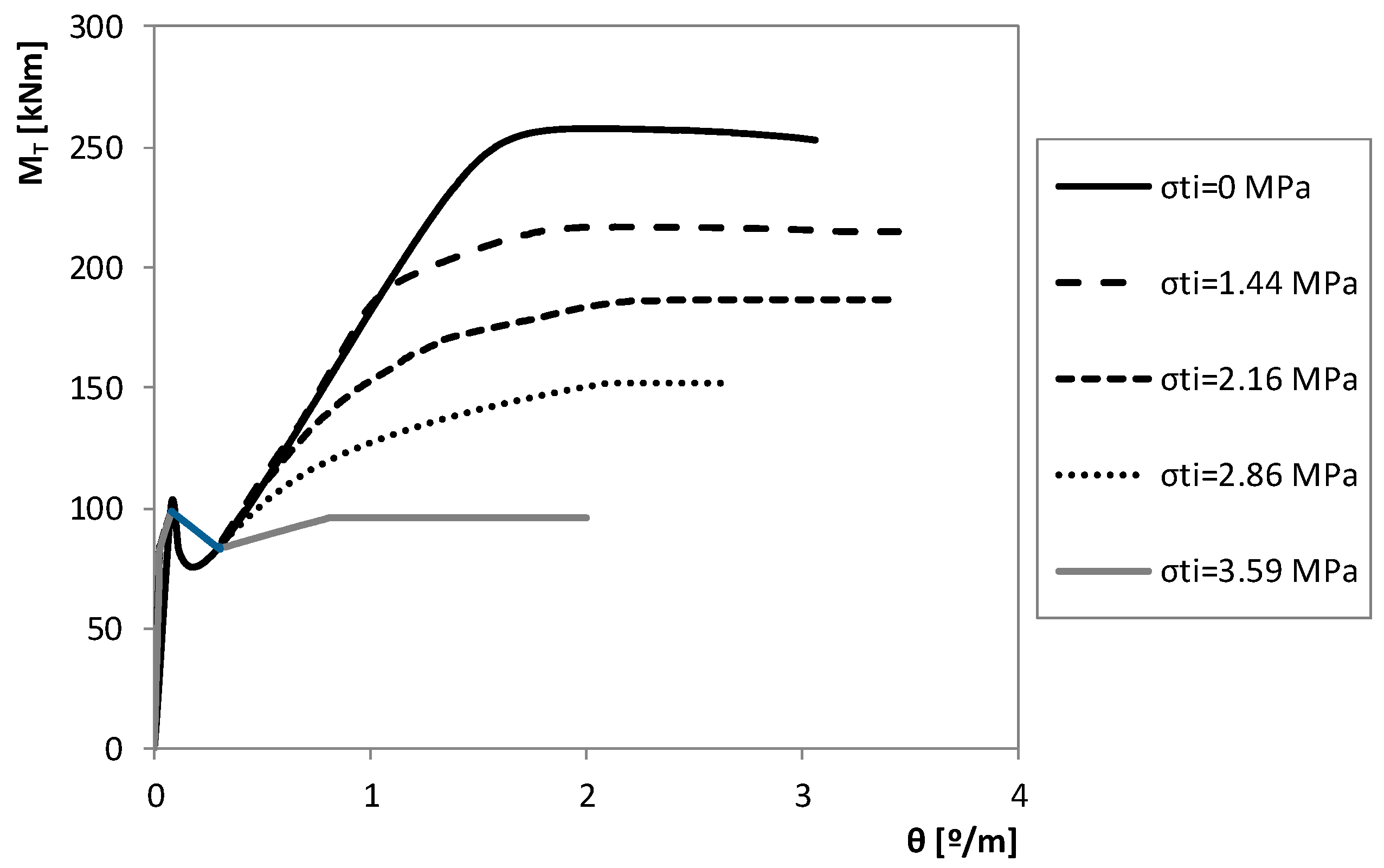
Figure 9 presents the theoretical
curves computed from GSVATM for beam A2 under torsion combined with the different tensile axial stress states
, presented in
Table 3. From
Figure 9, it can be observed that, unlike for
, as
increases, both the resistant torque and the torsional stiffness in the cracked state tend to decrease.
Regarding the cracking torque, reliable conclusions cannot be drawn, since GSVATM showed some convergence problems while computing the solution points for the theoretical
curves near the cracking point, in particular for torsion combined with the highest tensile stresses. For
(
Figure 9) this issue led to an atypical shape for the post-cracking curve, which must be regarded with some caution. However, for the level of axial stresses considered in this study, it is expected that the cracking torque slightly increases as
increases and decreases as
increases. In fact, a small increase in the cracking torque still can be observed for the lowest levels of
(
Figure 8). These convergence problems were reported in the literature [
11] and are related to the shape of the used
relationship to characterize the stiffened tensile concrete behavior (
Table 2), which incorporates a discontinuity in the peak stress point.
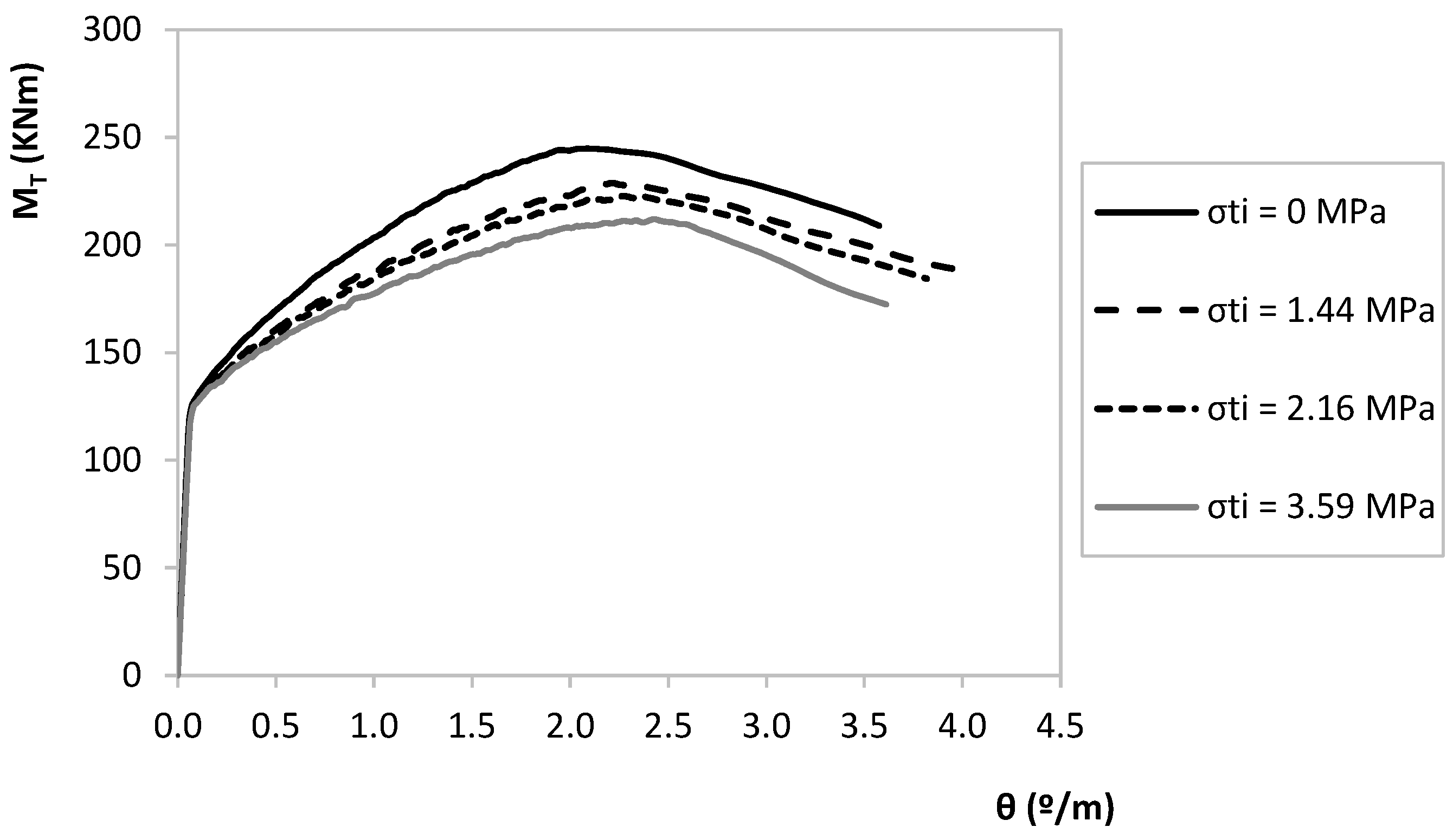
Figure 10 and
Figure 11 present the numerical
curves from FEM simulations for beam A2 under torsion combined with the same levels of uniform axial stress state considered in
Figure 8 and
Figure 9, respectively. From
Figure 10 and
Figure 11, it can be stated that the observed tendencies with respect to the resistant torque and corresponding twists, and also with the stiffness in the cracked stage, are similar to the ones previously reported from the results with GSVATM. With respect to the cracking torque, it is observed that it increases slightly as
increases and decreases slightly as
increases, as expected.
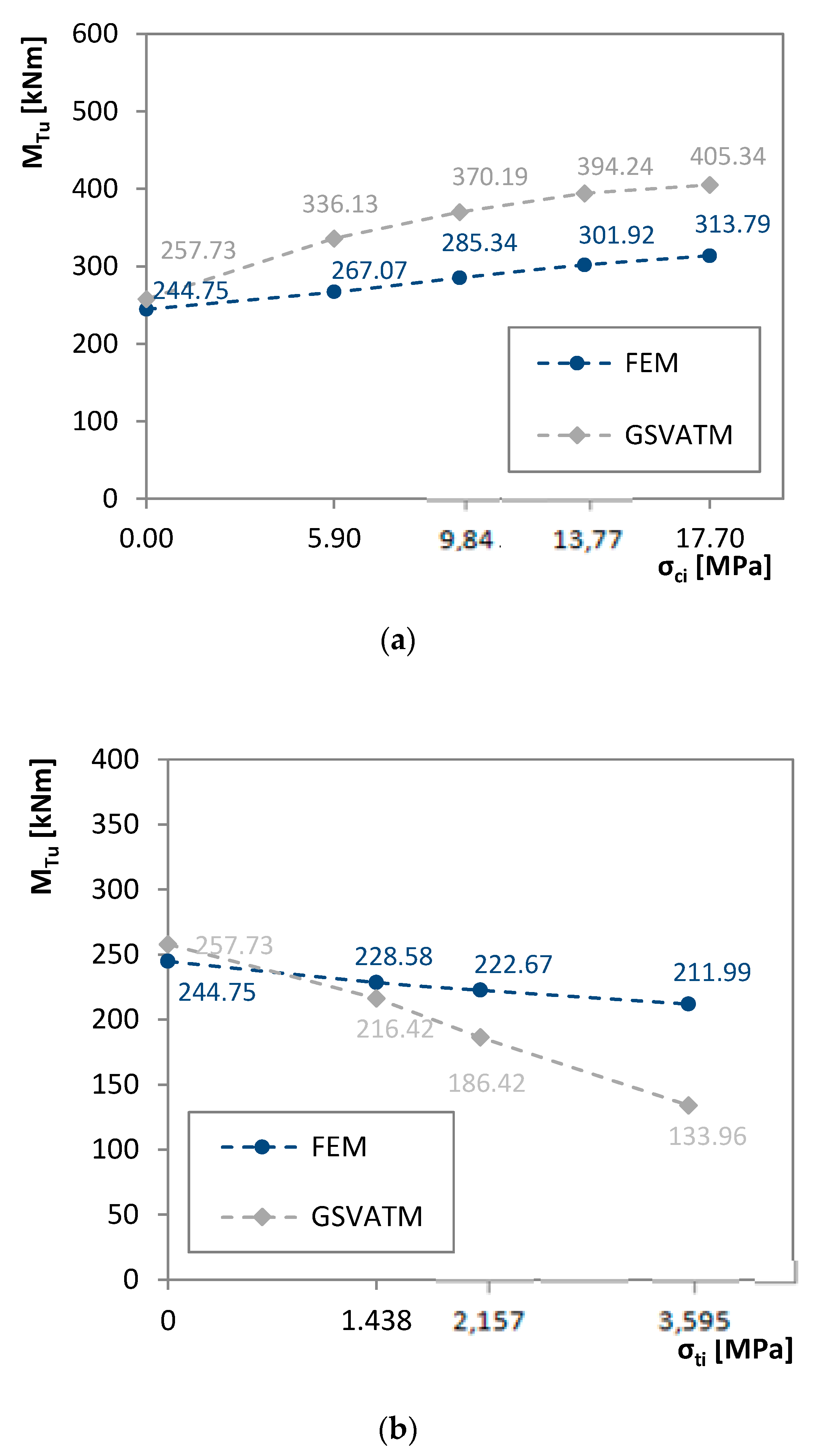
Figure 12a,b compare the variations of the theoretical and numerical resistant torques, which are summarized in
Table 4, for the different compressive and tensile stress states, respectively. From
Table 4 it is possible to observe and compare, for each simulation and for each level of axial stress state, the percentage variation of the resistant torque with respect to the same experimental one for beam A2 without axial stress state. Although some differences can be observed between the values for the theoretical predictions from GSVATM and FEM, the general trends agree. The observed differences result from the used base model to simulate the reference beam. While GSVATM is based on a 3D truss model, and is therefore a “non-continuous” model, the numerical model is based on a FEM model, which is a “continuous” model. Moreover, as previously stated, the FEM model was calibrated with beam A2 under pure torsion, since no experimental data of RC beams under torsion combined with axial forces was found in the literature. Despite this, the FEM results agree with the GSVATM ones as far as the general observed trends are concerned.
5. Conclusions
In this article, the GSVATM was extended to cover RC beams under torsion combined with external axial and centered force. The changes in the original GSVATM and the modified solution calculation procedure were presented. The theoretical predictions of the global behavior ( curves) of a reference RC beam under torsion combined with several external axial stress states, including compressive and tensile, where presented. The results were compared with the numerical results from FEM for the same reference beam and for the same loading cases.
From the obtained results, it can be stated that the trends related to the global behavior of the studied reference beam, either theoretically from GSVATM or numerically from FEM, agree.
The GSVATM for RC beams under torsion combined with external axial forces for RC beams constitutes a contribution to generalize the Space Truss Analogy. Research must continue in order to generalize the GSVATM for more general loading cases.


