LFTD: Transformer-Enhanced Diffusion Model for Realistic Financial Time-Series Data Generation

Abstract

Firm-level financial statement data form multivariate annual time series with strong cross-variable dependencies and temporal dynamics, yet publicly available panels are often short and incomplete, limiting the generalization of predictive models. We present Latent Financial Time-Series Diffusion (LFTD), a structure-aware augmentation framework that synthesizes realistic firm-level financial time series in a compact latent space. LFTD first learns information-preserving representations with a dual encoder: an FT-Transformer that captures within-year interactions across financial variables and a Time Series Transformer (TST) that models long-horizon evolution across years. On this latent sequence, we train a Transformer-based denoising diffusion model whose reverse process is FiLM-conditioned on the diffusion step as well as year, firm identity, and firm age, enabling controllable generation aligned with firm- and time-specific context. A TST-based Cross-Decoder then reconstructs continuous and binary financial variables for each year. Empirical evaluation on Korean listed-firm data from 2011 to 2023 shows that augmenting training sets with LFTD-generated samples consistently improves firm-value prediction for market-to-book and Tobin’s Q under both static (same-year) and dynamic ($\tau$ → $\tau +1$) forecasting settings and outperforms conventional generative augmentation baselines and ablated variants. These results suggest that domain-conditioned latent diffusion is a practical route to reliable augmentation for firm-level financial time series.

1. Introduction

Financial data analysis has long relied on traditional regression-based statistical models. However, as the need to handle nonlinearity, high dimensionality, and heterogeneous data simultaneously has grown, the use of machine- and deep-learning-based methods has expanded rapidly. By capturing complex structures more flexibly, these approaches can improve predictive accuracy relative to traditional models and partially automate risk assessment. As a result, they are now applied to a wide range of tasks, including firm valuation, bankruptcy prediction, deal-structure optimization, and earnings forecasting. At the same time, because financial statements are numerical, tabular data with time-series properties, model performance depends heavily on the quantity and quality of the training data. However, in practice, publicly available financial data typically cover only a limited set of firms and years and are characterized by frequent missing values and discontinuities in coverage, making it difficult to construct consistent long-term time series. This scarcity and fragmentation of data can substantially degrade the generalization performance of machine- and deep-learning models, which must learn highly complex patterns.

A widely used approach to alleviating data scarcity is data augmentation, which refers to techniques that generate additional training data by transforming or imitating existing samples. In domains such as computer vision and speech recognition, where strong structural regularities are present, a variety of augmentation methods—including rotation, cropping, noise injection, masking, and interpolation—have been used effectively [1,2]. More recently, research has moved beyond simple transformations to leverage deep generative models such as GANs [3,4], VAEs [5], and diffusion models [6,7,8]. These methods learn the statistical properties and structural patterns of the original data and can generate samples that exhibit both realism and diversity; in image and speech applications, they produce synthetic samples that are “sufficiently plausible” and closely aligned with the true data distribution.

Financial statements are a composite data type that combines a static tabular structure with time-series characteristics, and the interdependence among variables is tightly constrained by accounting identities and the definitions of financial ratios. Because these variables and ratios are tightly coupled, naïve augmentation can easily violate economically meaningful cross-variable relationships and disrupt temporal coherence. Therefore, for firm-level financial panels, effective augmentation must preserve both inter-variable structure and year-to-year dynamics; otherwise, financial consistency can be undermined.

Existing data-augmentation studies for financial statements typically adopt generative models developed for either tabular data, where firm–year records are treated as independent rows, or time-series data, where temporal dynamics are modeled but cross-variable accounting structure is only implicitly captured. As a result, prior approaches often struggle to simultaneously preserve variable-wise dependencies constrained by accounting identities and ratio definitions and temporal coherence across multiple years. Moreover, generating observations directly in the original variable space can amplify small inconsistencies into economically implausible samples. In addition, Transformers have recently been adopted mainly for prediction and classification on tabular or time-series financial data. However, their use for generative augmentation—especially for composite tabular–time-series financial statements—remains relatively underexplored.

To overcome these limitations, we propose a conditional Transformer–diffusion-based data augmentation model that simultaneously captures the tabular and time-series characteristics of financial data. Specifically, we first embed metadata, such as year and firm identifiers, together with continuous and categorical financial variables, and then use the FT-Transformer [9] to construct column embeddings that reflect inter-variable relationships. Because the FT-Transformer applies self-attention over column tokens, it does not directly model dependencies on temporal order or sequence length. We therefore employ a Time Series Transformer (TST) [10] to capture temporal dynamics and interactions among variables and to construct a conditioning representation sequence. We call our model Latent Financial Time-Series Diffusion (LFTD).

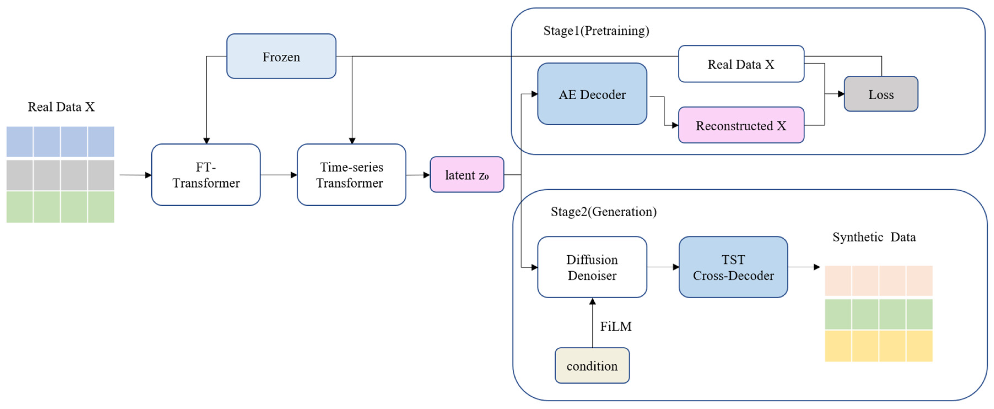
In the LFTD, the Transformer module takes this conditioning representation sequence, along with firm identifiers, positional encodings, and year information, as conditioning inputs and maps them to a latent vector. The diffusion denoiser is trained to reconstruct the conditioning representation sequence from this latent representation. After training, given a user-specified firm identifier and sequence of years, we encode them through the same FT-Transformer and TST pipeline to obtain a conditioning representation sequence and then perform a diffusion-based reconstruction process conditioned on this sequence to generate new multivariate financial time series that simultaneously exhibit financial consistency and temporal coherence.

The main contributions of this study are as follows:

• Domain-consistent augmentation: We present a structure-preserving augmentation framework for multivariate firm-level financial time series that explicitly targets cross-variable dependencies and reduces violations of economically meaningful relationships among financial indicators.
• Dual-dependency representation: We introduce an encoding design that disentangles and captures temporal evolution across years and variable-wise interactions within each firm–year record, producing compact latents for generation.
• Controllable conditional diffusion: We develop a conditional Transformer–diffusion generator operating in latent space, conditioned on year and firm identity to enable controllable synthesis with temporal coherence.

The remainder of this paper is organized as follows. Section 2 reviews related work. Section 3 describes the proposed method in detail. Section 4 presents quantitative evaluations focusing on the statistical properties and predictive performance of the generated data. Section 5 concludes and discusses directions for future research.

2. Related Work

2.1. Financial Data Analysis with Machine Learning and Deep Learning

Financial statements are key instruments for assessing a firm’s financial soundness and operating performance, and they have traditionally been analyzed using statistical methods such as regression and discriminant analysis [11]. More recently, machine-learning models including Random Forest, XGBoost, and SVM have been introduced for tasks such as bankruptcy prediction and profitability analysis, enabling more effective modeling of complex nonlinear relationships among variables [12,13,14]. For example, Son et al. applied machine-learning models including XGBoost to predict bankruptcy risk for Korean companies and reported an average improvement of about 17% in AUC over existing baseline models such as logistic regression [15]. Similarly, Zhou et al. (2020) proposed a CNN-based model for personal loan default prediction using the Lending Club dataset and reported higher AUC/accuracy than traditional models such as SVM, Bayes, and Random Forest, highlighting the benefit of capturing nonlinear relationships [16]. However, most of these studies rely on static data from a single point in time or, at most, year-by-year snapshots, and thus have limited ability to fully exploit temporal continuity. Recurrent neural networks such as LSTM and GRU [17,18] have seen some adoption, but they remain insufficient for learning long-term dependencies across years, are structurally difficult to parallelize, and are not well-suited to handling tabular structures such as financial statements, which combine categorical and numerical variables. To overcome these limitations, Transformer-based models have recently attracted growing attention. TabTransformer [19] and FT-Transformer [9] exhibit strong representation-learning performance on tabular data with mixed categorical and numerical features. Huang et al., for instance, applied TabTransformer to a loan default prediction dataset and reported a 3.1% improvement in AUC compared with a Random Forest baseline. In the time-series domain, models such as TST (Time Series Transformer) [10] and TFT (Temporal Fusion Transformer) [20] have been proposed. Lim et al. (2021) showed that TFT improves long-term forecasting accuracy over LSTM for electricity demand prediction, while also providing interpretable variable importance [20].

2.2. Tabular and Time-Series Data Augmentation

Data augmentation is a key technique for improving model generalization, and tabular and time-series data require distinct approaches because of their different structural characteristics. For tabular data, methods such as SMOTE [21], CTGAN [22], TableGAN [23], and VAE-based models [5] are widely used, with a primary focus on preserving the underlying statistical structure among variables. For example, CTGAN, proposed by Xu et al. (2019), demonstrated more stable distributional fidelity than conventional GANs on the UCI Adult Income dataset. In contrast, time-series augmentation must simultaneously account for temporal dynamics and joint relationships among variables [22]. Methods such as TimeGAN [24], T-CGAN [25], and TS-Augment [26] have been proposed for this purpose. Yoon et al. applied TimeGAN to financial time series and showed that the generated samples preserve autocorrelation structures similar to those of the original data [24]. However, existing approaches are typically specialized for either tabular or time-series data alone and therefore face limitations when applied to composite data such as financial statements, which embody both structures. Time-series data possess a distinctive structure in which temporal dependencies and cross-variable correlations coexist, so naive augmentation strategies can easily introduce semantic distortions. In particular, both the magnitude of values and their evolution over time (i.e., ordering and trends) are important for interpretation, making it difficult to directly adopt augmentation schemes designed for static data. Um et al. (2017), analyzing sensor data from Parkinson’s disease patients, showed that traditional augmentation methods such as noise injection and temporal shifting can actually degrade predictive performance and interpretability [27]. Zerveas et al. likewise reported that simple resampling strategies may compromise clinical meaning in medical time-series data. These findings suggest that arbitrary transformations can similarly distort the economic meaning of financial data, underscoring the need for sophisticated generative augmentation methods that preserve both structural consistency and temporal dynamics [10].

2.3. Diffusion-Based Time-Series and Tabular Data Generation

Diffusion models have emerged as powerful generative methods across a wide range of domains—including images, text, and time series—because of their robustness in learning complex data distributions. A representative example is the Denoising Diffusion Probabilistic Model (DDPM), which generates samples by gradually corrupting data with noise and then learning the reverse denoising process [5]. Subsequent extensions, such as score-based and conditional diffusion models, have broadened their applicability to various tasks [6]. In the time-series domain, CSDI (Conditional Score-Based Diffusion Model for Imputation) by Tashiro et al. (2021) [28] is a representative approach; on electricity consumption data, it achieved more than a 20% improvement in imputation performance over LSTM-based baselines. For tabular data, TabDDPM by Kotelnikov et al. (2022) [29] demonstrated lower Kolmogorov–Smirnov statistics than VAE- and CTGAN-based models on credit risk datasets, indicating improved statistical fidelity of the generated samples.

Nonetheless, most existing diffusion-based models are tailored to either static tabular data or pure time-series data, making them difficult to apply directly to composite datasets such as financial statements, where tabular and time-series structures are tightly coupled. To address this gap, the present study proposes a diffusion model that uses financial embeddings derived from FT-Transformer and TST as conditioning signals, with the aim of generating realistic, finely detailed financial time series that jointly satisfy statistical consistency and temporal coherence.

3. Methodology

In this study, we focus on generating realistic synthetic firm-level financial statement time series that preserve both cross-sectional (within-year) relationships among variables and long-term (across-year) temporal dynamics. Our objective is to develop a conditional generative model that learns a stable latent representation of such data and produces high-fidelity synthetic sequences for downstream analysis and simulation. To this end, we propose a conditional time-series generation model, Latent Financial Time-Series Diffusion (LFTD), which generates realistic synthetic financial data from numerical time-series observations in the form of financial statements. Because financial statement data exhibits a complex structure that combines a static tabular format of yearly observations and long-term temporal dynamics accumulated at the firm level, effectively learning such data requires latent representation learning that simultaneously captures both the intra-year inter-variable structure and the inter-year time-series structure. To this end, the proposed LFTD consists of three key modules organized in a two-stage training framework.

In the first stage, a time-series encoder that combines an FT-Transformer and a Time Series Transformer (TST) embeds firm-level financial time series into a latent representation space. Specifically, the FT-Transformer learns the structural relationships among the continuous and binary numerical variables contained in each year’s financial statements, summarizing the annual financial status into a high-dimensional vector. These yearly latent vectors are then fed into the TST, which models long-term financial dynamics and temporal dependencies at the firm level. This stage is pre-trained in an autoencoder manner, forming a stable latent financial time-series representation that reflects the structural characteristics of financial time series.

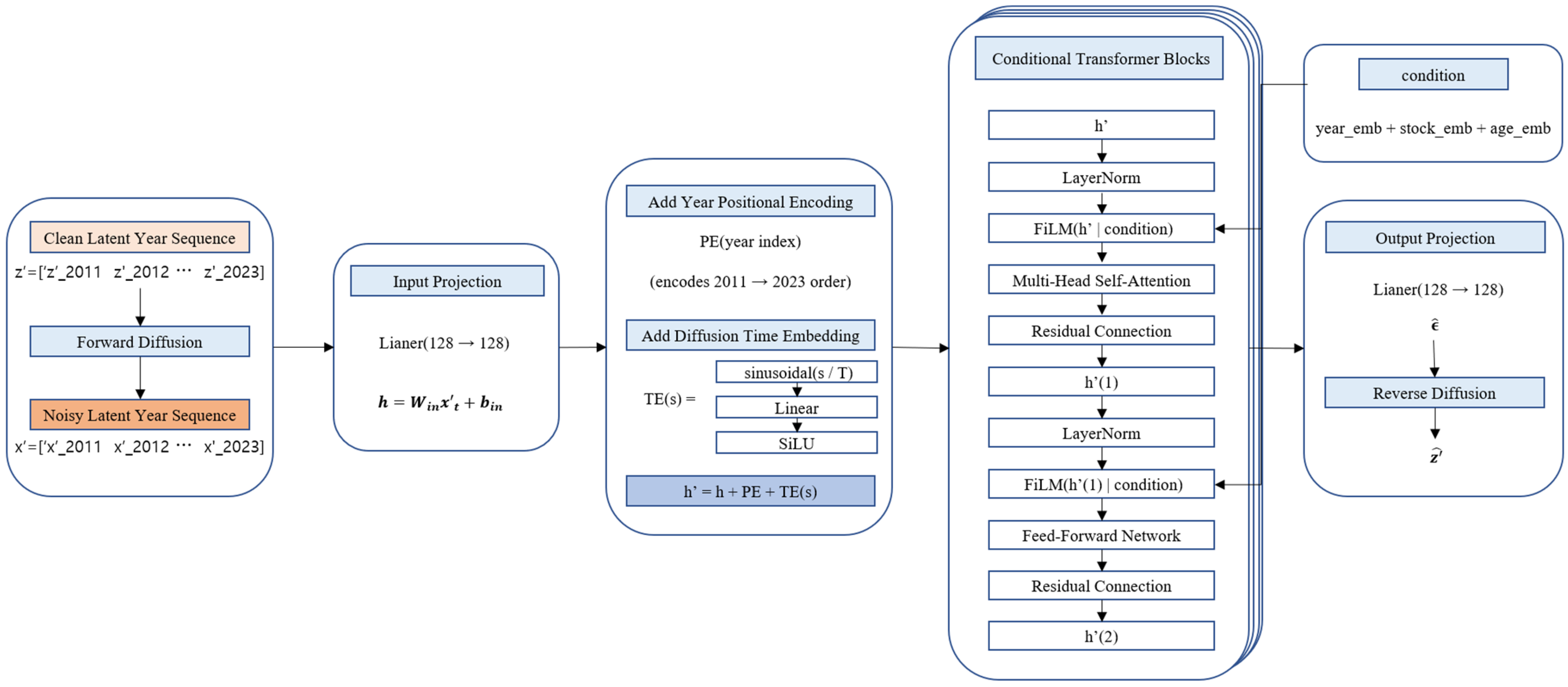
In the second stage, a conditional diffusion model with a Transformer-based denoiser is trained using the latent time-series representations obtained from the pre-trained encoder. The diffusion process is performed over the entire latent time series at the firm level, and the denoising in the reverse diffusion steps is conditioned not only on the diffusion time step but also on year, firm ID, and firm age. These conditioning signals are injected into each layer of the Transformer denoiser via FiLM (Feature-Wise Linear Modulation), enabling condition-aware generation of latent time series.

Finally, the latent time series recovered through the reverse diffusion process is decoded back into the original financial variable space via a TST-based Cross-Decoder. This decoder performs cross-attention over the latent time-series representations using learnable query tokens, reconstructing the yearly financial variables into a temporally consistent time-series structure. Through this design, the proposed model can generate synthetic financial time-series data that satisfy firm-level and year-level conditions. Figure 1 provides an overview of the full architecture and training pipeline of the proposed LFTD model.

3.1. Dataset Description

The dataset used in this study is constructed from the financial statements of Korean listed firms and contains consecutive annual observations from 2011 to 2023, for a total of 13 years. Each firm is identified at the entity (stock) level, and for each year (YEAR), key financial indicators and accounting characteristics are recorded. For the final analysis, we restrict the sample to firms that are observed without missing values for the full 13-year period. Following the data-collection and preprocessing pipeline described in our KoTaP [30], we retrieved most raw annual financial-statement items (e.g., assets, liabilities, sales, cash-flow items, pretax income, and income tax expense) from the Financial Supervisory Service’s DART system via the OpenDART API and standardized them into a firm–year panel. Any “manual” steps refer only to limited human-in-the-loop procedures such as maintaining the account-to-variable mapping dictionary, resolving rare ambiguous identifiers, and conducting spot-check validation against original filings; importantly, no financial-statement numbers were manually entered. After merging sources by firm identifier and fiscal year and applying deterministic cleaning rules and sample filters (e.g., denominator/eligibility checks and missing-value handling), we restricted the analysis to a balanced panel with complete observations for all 13 years (2011–2023). The final dataset used in this study contains 1284 unique firms and 16,692 firm–year observations. This dataset is not identical to KoTaP, although the overall construction procedure is consistent.

Table 1. Definition of variables.

Variables	Definition of Variables
OWN	The largest shareholder’s share ratio [31]
FORN	Foreign investors’ share ratio [32]
SIZE	Natural logarithmic value of total assets
LEV	Debt-to-equity ratio
CUR	Current ratio = Current assets/Current liabilities [33]
GRW	Sales growth rate [34]
ROA	Return on assets = Net income/Beginning total assets
ROE	Return on equity = Net income/Beginning shareholders’ equity
CFO	Operating cash flow ratio
PPE	Proportion of tangible assets subject to depreciation [35]
INVREC	Ratio of inventory and accounts receivable
MB	MB = Market value of equity at year-end/Book value of equity at year-end [36]
TQ	Tobin’s Q = (Total liabilities + Market value of equity)/Total assets at year-end
BIG4	A dummy variable indicating whether the auditor belongs to a Big 4 accounting firm [37]
LOSS	A dummy variable equal to 1 if the firm reports a net loss in year $\tau$ (Net ${\mathrm{i}\mathrm{n}\mathrm{c}\mathrm{o}\mathrm{m}\mathrm{e}}_{\tau }$ < 0), and 0 otherwise
YEAR	Calendar year of observation, serving as a temporal index for the firm-level time series
STOCK_ID	Unique firm identifier at the stock level, used to distinguish individual firms in the panel data
AGE	Firm age, measured as the number of years since the firm’s establishment

summarizes the definitions of the variables included in the dataset. The variables can be broadly classified into continuous financial variables and binary indicators. The continuous variables include insider ownership (OWN), foreign ownership (FORN), firm size (SIZE), leverage ratio (LEV), current ratio (CUR), sales growth (GRW), return on assets (ROA), return on equity (ROE), operating cash flow ratio (CFO), property, plant and equipment ratio (PPE), inventory and receivables ratio (INVREC), market-to-book ratio (MB), and Tobin’s Q (TQ). The binary variables indicate whether the external auditor belongs to a Big 4 accounting firm (BIG4) and whether the firm reports a net loss in the current year (LOSS).

In addition, the dataset includes three auxiliary variables that are not directly generated by the model but are used to define the panel structure and provide contextual information: the calendar year (YEAR) as a temporal index, a stock-level firm identifier (STOCK_ID), and firm age (AGE), which is treated as a firm-specific conditioning variable. All continuous main input variables are normalized prior to model training. This data design enables the model to capture both temporal patterns within firms and cross-sectional heterogeneity across firms.

3.2. Year-Wise Financial Feature Embedding

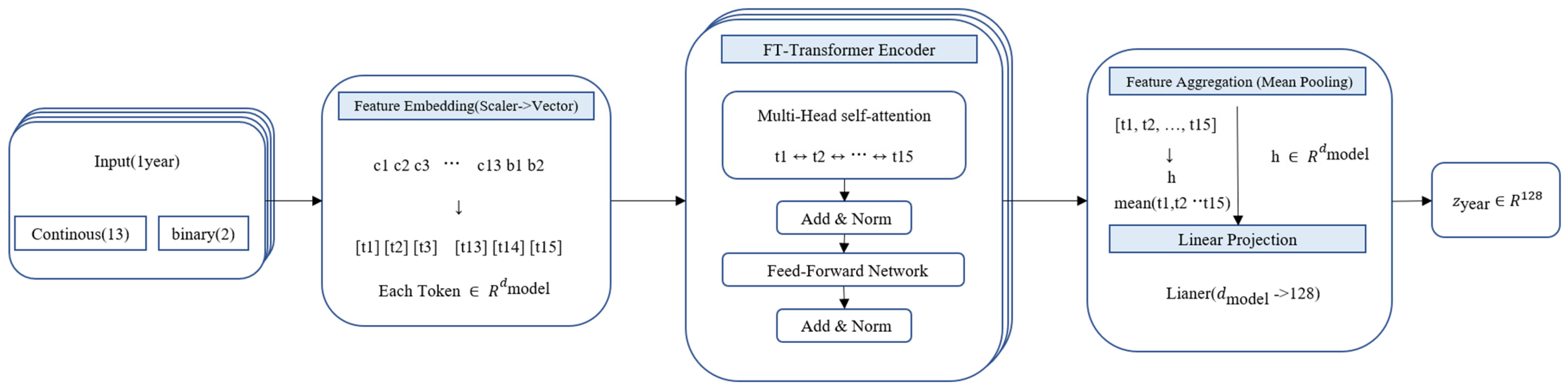
In this study, we consider firm-level financial time-series data, where each firm has consecutively observed financial statement information for a total of 13 years from 2011 to 2023. The financial data observed in each year $\tau$ are represented as a structured vector consisting of 13 continuous variables and 2 binary variables. In this section, we define the process of embedding these year-level financial inputs into a single latent vector.

We define the financial input firm n at year $\tau$ as follows: $x_{n,\tau }=\left[c_{n,\tau ,1},\dots ,c_{n,\tau ,13},b_{n,\tau ,1},b_{n,\tau ,2}\right]\in {\mathbb{R}}^{15}$ where $c_{n,\tau ,i}$ denotes the i-th continuous financial variable and $b_{n,\tau ,i}$ denotes the i-th binary financial variable. Each firm has a financial time series over 13 consecutive years, denoted as $\left[x_{n,1},x_{n,2},\dots ,x_{n,13}\right]$.

3.2.1. Year-Wise Feature Tokenization

Because year-level financial data have a structured format in which inter-variable interactions are crucial, it is difficult for simple linear transformations or time-series models alone to adequately capture the intra-year structural relationships. To address this, we employ an FT-Transformer to embed each year’s financial input into a latent space [9].

The FT-Transformer is a Transformer-based model that treats each financial variable as an independent token and learns interactions among variables through a self-attention mechanism [9,26]. As shown in Equation (1), the year $\tau$, firm n and financial input $x_{n,\tau }$ are decomposed into variable-wise components, each of which is mapped into a vector space via an independent embedding function.

$$e_{n,\tau ,i}=f_i\left(x_{n,\tau ,i}\right),\hspace{1em}i=1,\dots ,15$$

(1)

Here, $f_i(\cdot )$ is a learnable linear mapping corresponding to variable $i$. As a result, year $\tau$ is represented as the following sequence of variable tokens: $E_{n,\mathsf{\tau }}=\left[e_{n,\tau ,1},\dots ,e_{n,\tau ,15}\right]\in {\mathbb{R}}^{15\times { d}_{model}}$.

3.2.2. FT-Transformer Encoding and Year-Level Aggregation

The variable-token sequence $E_{n,\tau }$ is used as the input to the FT-Transformer encoder, and through self-attention, it is transformed into contextualized representations that reflect the relative importance and correlations among variables within the year [9]. The encoder output tokens are then aggregated into a single year-level representation via mean pooling, as shown in Equation (2).

$$h_{n,\mathsf{\tau }}={\displaystyle \frac{1}{N}}\sum _{i=1}^N{e}_{n,\tau ,i}$$

(2)

Here, $N$ denotes the number of variable tokens, and, in this case, N = 15. Then, as shown in Equation (3), the final year embedding is obtained via a linear projection.

$$z_{n,\tau }=W{h}_{n,\tau }+b, z_{n,\tau }\in {\mathbb{R}}^{128}$$

(3)

In this way, each year’s financial input is transformed into a fixed-length latent vector that reflects the structural interactions among variables within the year. Figure 2 schematically illustrates the overall process by which year-level financial inputs are converted into year embeddings through variable tokenization, the FT-Transformer encoder, and aggregation. The resulting year embeddings $z_{n,\tau }$ are then used as inputs for learning firm-level temporal structure and are fed into the Time-Series Transformer module described in the next section.

3.3. Representation Learning via Time Series Transformer

In this section, we describe how the year-level embeddings $z_{n,\tau }\in {\mathbb{R}}^{128}$ obtained in Section 3.2 are organized as a sequence along the time (year) axis to learn a firm’s long-term financial dynamics and inter-temporal dependencies. For firm $n$, we denote the sequence of T yearly embeddings as $Z_n=\left[z_{n,1},z_{n,2},\dots ,z_{n,13}\right]\in {\mathbb{R}}^{\mathrm{T}\times 128}$. This sequence is then used as the input to the Time Series Transformer (TST) encoder. Through self-attention, the TST directly models interactions between any two time steps, enabling it to learn long-range dependencies such as trends, turning points, and lagged effects [10,38].

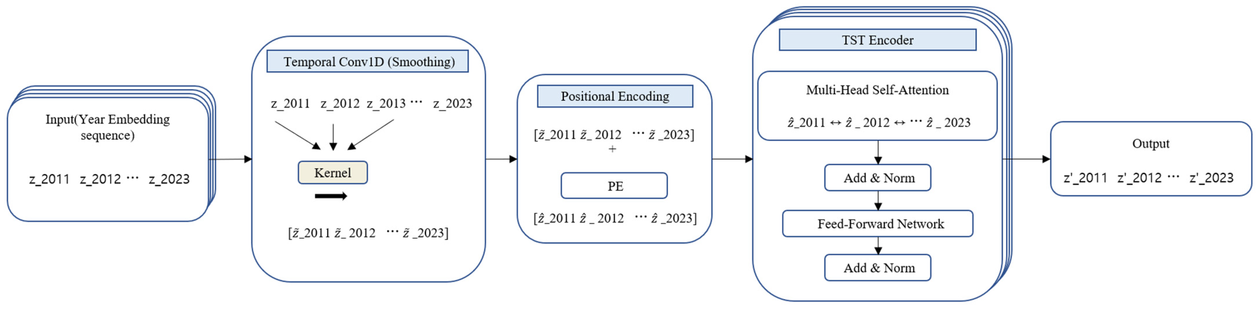
3.3.1. Temporal Smoothing via 1D Convolution

The year-embedding sequence $Z$ is first passed through a one-dimensional convolution (1D convolution) layer applied along the year axis. This layer aggregates local context across adjacent years, helping to smooth short-term noise or abrupt fluctuations and to form a more stable time-series representation. The resulting output sequence $\tilde{Z}$ is expressed as Equation (4).

$$\tilde{Z}=\mathrm{C}\mathrm{o}\mathrm{n}\mathrm{v}1\mathrm{D}\left(Z\right)$$

(4)

3.3.2. Sinusoidal Positional Encoding

Because a Transformer does not inherently encode sequential order, we add sine–cosine positional encoding to explicitly inject year ordering and relative distance information. Let the positional encoding matrix be $P\in {\mathbb{R}}^{13\times 128}$; then, the input to the TST is constructed as shown in Equation (5).

$$H^{\left(0\right)}=\tilde{Z}+P$$

(5)

In this case, each element of $P$ follows the standard sinusoidal encoding scheme [38].

3.3.3. Transformer Encoder for Temporal Dependency Modeling

The TST consists of $L$ Transformer encoder blocks, where each block is composed of multi-head self-attention and a position-wise feed-forward network (FFN), along with residual connections and layer normalization [10,38]. Let $H^{\left(l-1\right)}$ denote the input to the $l$-th block and $H^{\left(l\right)}$ its output; then $H^{\left(l\right)}$ can be expressed as shown in Equation (6).

$$H^{\left(l\right)}={\mathrm{TSTBlock}}^{\left(l\right)}\left(H^{\left(l-1\right)}\right), l=1,\dots ,L$$

(6)

Through self-attention, the representation at each time step can reference information from all other time steps as a weighted sum, where the weights reflect the importance of inter-temporal interactions [38]. As a result, the final output $Z^{\prime }=H^{\left(L\right)}\in {\mathbb{R}}^{13\times 128}$ is a refined latent time-series representation in which each year-level embedding is contextualized by the entire sequence.

This $Z^{\prime }$ simultaneously captures intra-year variable interactions (via the FT-Transformer) and inter-year temporal dynamics (via the TST). It is subsequently used as a latent-space input for the reconstruction learning in Stage 1 and for the conditional diffusion model in Stage 2. Figure 3 schematically illustrates the process by which the year-level embeddings are transformed into $Z^{\prime }$ through Conv1D, positional encoding, and the TST encoder.

3.4. Latent Space Pretraining via Autoencoder (Stage 1)

For a conditional diffusion model to be stably trained in the latent space, the latent time-series representations used as diffusion inputs must sufficiently preserve the original financial information. To this end, we construct the FT–TST encoder (Section 3.2 and Section 3.3) in an autoencoder framework and conduct Stage 1 pre-training [39]. The goal of Stage 1 is not generation, but rather the establishment of an information-preserving latent space that is suitable for subsequent diffusion training.

3.4.1. Decoder Architecture for Reconstruction

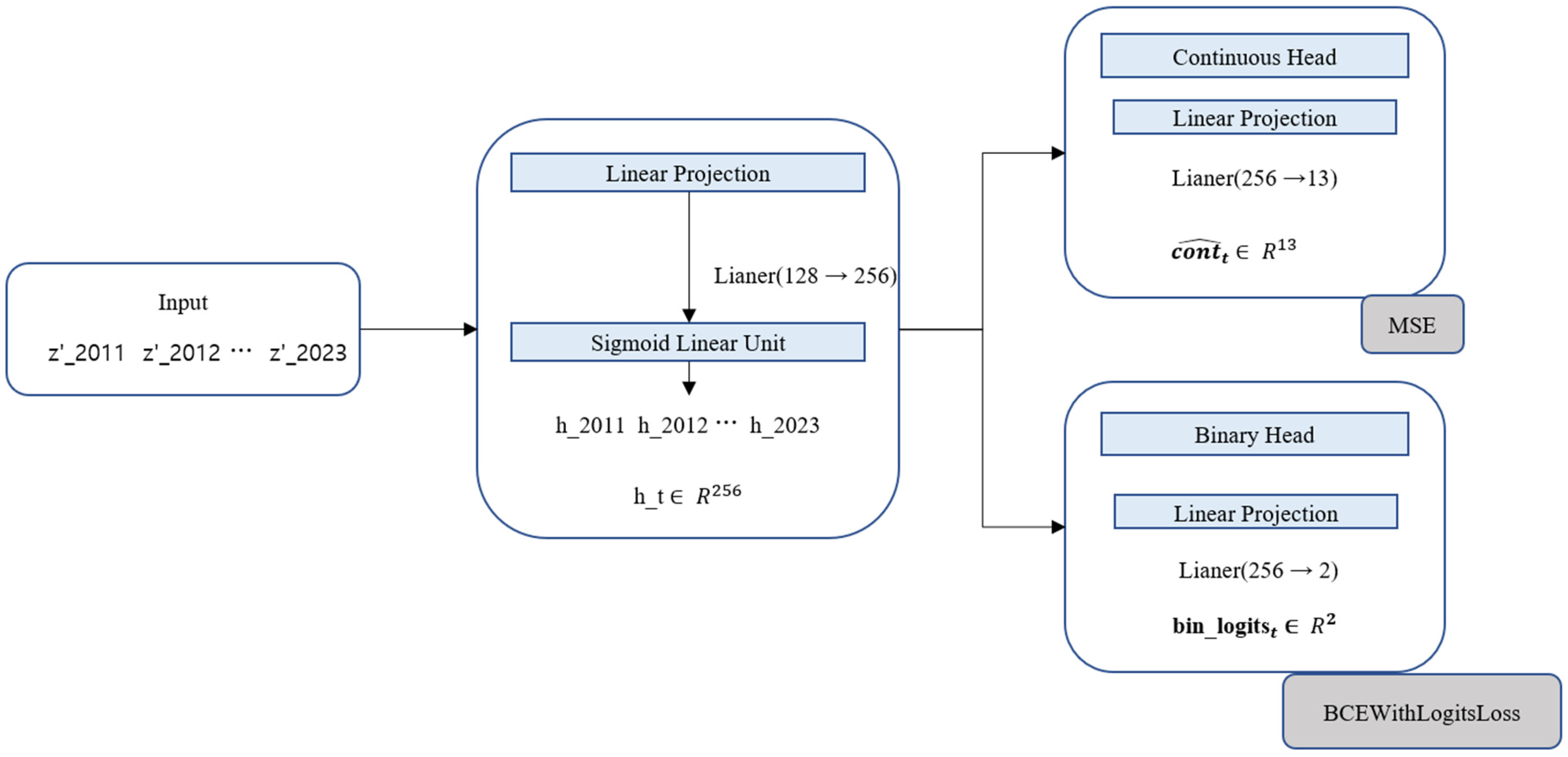
In Stage 1, we train a decoder to reconstruct the original financial variables (13 continuous and 2 binary) from the TST output latent time series $Z^{\prime }\in {\mathbb{R}}^{13\times 128}$. The decoder first maps each latent vector into a shared hidden space and then branches into separate output heads for continuous and binary variables. Let $z_{n,\tau }^{\prime }$ denote the latent vector of firm n at year $\tau$; the shared transformation is given in Equation (7).

$$u_{n,\tau }=\varphi \left(W_{sh}{z}_{n,\tau }^{\prime }+b_{sh}\right)$$

(7)

Here, $\varphi (\cdot )$ denotes a nonlinear activation function (SiLU). The reconstructed continuous variables ${\widehat{c}}_{n,\tau }\in {\mathbb{R}}^{13}$ and the binary logits ${\widehat{b}}_{n,\tau }^{\mathit{logit}}\in {\mathbb{R}}^2$ are then computed as in Equation (8), respectively.

$${\widehat{c}}_{n,\tau }=W_c{u}_{n,\tau }+b_c,\hspace{1em}\hspace{1em}{\widehat{b}}_{n,\tau }^{\mathit{logit}}=W_b{u}_{n,\tau }+b_b$$

(8)

3.4.2. Reconstruction Objectives

The reconstruction loss for the continuous variables is computed using the mean squared error (MSE), as given in Equation (9).

$$L_{cont}={\displaystyle \frac{1}{D_c}}{\sum }_{k=1}^{D_c}({\widehat{c}}_{n,\tau ,k}-c_{n,\tau ,k}{)}^2$$

(9)

In this case, dimension $D_c$ is 13.

The binary variables are trained using the logit-based binary cross-entropy loss (BCE with logits). Equation (10) is given as follows.

$$L_{bin}={\displaystyle \frac{1}{D_b}}{\sum }_{j=1}^{D_b}\left[\mathit{max}\left({\widehat{b}}_{n,\tau , j}^{\mathit{logit}},0\right)-{\widehat{b}}_{n,\tau , j}^{\mathit{logit}}{b}_{n,\tau ,j}+log(1+\mathit{exp}\left(-\left|{\widehat{b}}_{n,\tau , j}^{\mathit{logit}}\right|\right))\right]$$

(10)

where $D_b$ is 2. The overall Stage 1 objective function is defined as a weighted sum of the two losses, as shown in Equation (11).

$$L_{AE}=L_{cont}+{\lambda }_{bin}{L}_{bin}$$

(11)

Here, ${\lambda }_{\mathrm{bin}}$ is a hyperparameter that controls the balance between the reconstruction losses for the continuous and binary variables.

3.4.3. Role of Stage 1 Pretraining

Through this reconstruction-based training, the encoder learns latent representations that not only compress the input but also preserve the structural relationships among financial variables and the underlying temporal dynamics [39]. Consequently, the encoder trained in Stage 1 enables the Stage 2 conditional diffusion model to perform stable denoising in the latent space, and it serves as a foundation for reducing information loss when reverse-diffusion samples are decoded back into the original variable space. Figure 4 schematically illustrates the autoencoder pre-training framework, where the decoder branches into continuous and binary output heads.

3.5. Conditional Latent Diffusion with Transformer-Denoiser

In Stage 2 of this study, the diffusion process is performed directly on the latent time-series representations produced by the FT–TST encoder. Specifically, we use the time-series latent representation $Z_n^{\prime }=\left[z_{n,1}^{\prime },z_{n,2}^{\prime },\dots ,z_{n,T}^{\prime }\right]$ obtained in Section 3.3 as the reference state for the diffusion process, and generate new latent time series through forward diffusion and reverse diffusion. By conducting diffusion in the latent space, we can model the high-dimensional and complex distribution of the original financial data in a more stable and efficient manner [5,6].

3.5.1. Forward Diffusion in Latent Space

In the forward diffusion stage, Gaussian noise is gradually injected into the latent time series $Z_n^{\prime }$, producing noisy states $Z_s$ for diffusion steps $\mathrm{s}=1, 2,\dots ,S$. This process follows the DDPM framework, where the noise injection at each step is defined as in Equation (12).

$$Z_s=\sqrt{{\overline{\alpha }}_s}{Z}_n^{\prime }+\sqrt{1-{\overline{\alpha }}_s}\hspace{0.17em}ϵ, ϵ\sim \mathcal{N}\left(0,I\right)$$

(12)

Here, ${\overline{\alpha }}_s={\prod }_{i=1}^s{\alpha }_i$ is the cumulative attenuation coefficient, and $\left\{{\alpha }_s\right\}$ follows a predefined noise schedule. As the diffusion step increases, $Z_s$ gradually approaches pure Gaussian noise [5].

3.5.2. Transformer-Denoiser Architecture

In the reverse diffusion stage, we use a Transformer-based denoiser to learn how to progressively recover the original latent structure from the noisy latent time series $Z_{n,s}$. By adopting a self-attention-based Transformer architecture, the denoiser models global interactions across the entire sequence and effectively captures long-range temporal dependencies [10,38].

The noisy latent time series $Z_{n,s}$ is mapped to the denoiser’s model dimension via a linear projection, as shown in Equation (13).

$$H_{n,s}=W_{\mathrm{in}}{Z}_{n,s}+b_{\mathrm{in}}$$

(13)

Afterward, a year-index-based positional encoding is added to reflect the yearly order, and the diffusion step $s$ is transformed into a sine–cosine time embedding and injected into the input. The final denoiser input is constructed as $H_{n,s}+\mathrm{P}{\mathrm{E}}_{\mathrm{year}}+\mathrm{TE}\left(s\right)$ In this study, we adopt conditional diffusion to improve controllability and realism in the generation process. Year information, firm identifier, and firm age are each represented via embeddings, and these condition embeddings are concatenated into a single condition vector. This condition vector is injected into each layer of the Transformer denoiser using FiLM (Feature-Wise Linear Modulation) [40]. FiLM applies a linear modulation to the denoiser’s hidden representation $h$ as in Equation (14), where $\mathbf{c}$ denotes the combined conditioning information (year, firm ID, and firm age). Here, $\gamma (\cdot )$ and $\beta (\cdot )$ are learnable functions. Through this mechanism, conditioning signals directly influence the denoiser’s internal computations, enabling the model to learn latent time-series generation that reflects firm-specific and year-specific characteristics [28,40].

$$\mathrm{FiLM}\left(h∣c\right)=\gamma \left(c\right)\odot h+\beta \left(c\right)$$

(14)

The Transformer denoiser consists of multiple Transformer blocks, each comprising multi-head self-attention and a feed-forward network, along with residual connections and layer normalization [38]. With this architecture, the denoiser predicts noise at each diffusion step by considering the context of the entire latent time series.

3.5.3. Training Objective with SNR-Weighted Loss

During training, we design the loss function such that the denoiser accurately predicts the injected noise $ϵ$ at each diffusion step. Given the denoiser’s noise prediction ${\widehat{ϵ}}_{\theta }\left(Z_{n,s},s,c\right)$, we minimize the following objective [5].

In addition, we apply an SNR (signal-to-noise ratio)-based weighting scheme across diffusion steps to mitigate training instability in high-noise regimes [6,28]. This design encourages stable learning throughout the diffusion trajectory and helps preserve the long-term structure of the latent time series. Diffusion loss is defined in Equation (15).

$${\mathcal{L}}_{\mathrm{d}\mathrm{i}\mathrm{f}\mathrm{f}}=E_{s,ϵ}\left[{\mathrm{w}}_s·\left|\right|ϵ-{\widehat{ϵ}}_{\theta }\left(Z_{n,s},s,c\right)\right|{|}^2]$$

(15)

Here, $w_s$ denotes $\min \left(SN{R}_s, \gamma \right)$ and $SN{R}_s$ is defined as ${\overline{\alpha }}_s$/$(1-{\overline{\alpha }}_s)$.

3.5.4. Sampling via Reverse Diffusion

During generation, we perform reverse diffusion starting from pure Gaussian noise using the trained Transformer denoiser. At each step, the predicted noise is substituted into the reverse diffusion update, repeatedly applying $Z_{n,s}$→$Z_{n,s-1}$ to ultimately recover a latent time series with the same structure as $Z^{\prime }$ [5,6]. The generated latent time series is then transformed back into the original financial variable space through the decoder. Figure 5 schematically illustrates the conditional diffusion process in the latent time-series space and the overall architecture of the Transformer denoiser.

3.6. Cross-Decoder and Financial Time-Series Generation

Through the conditional latent diffusion process described in the previous section, the model obtains denoised latent time-series representations after reverse diffusion. In this section, we explain how the recovered latent time series is transformed into the original financial variable space, ultimately generating firm-level financial time-series data.

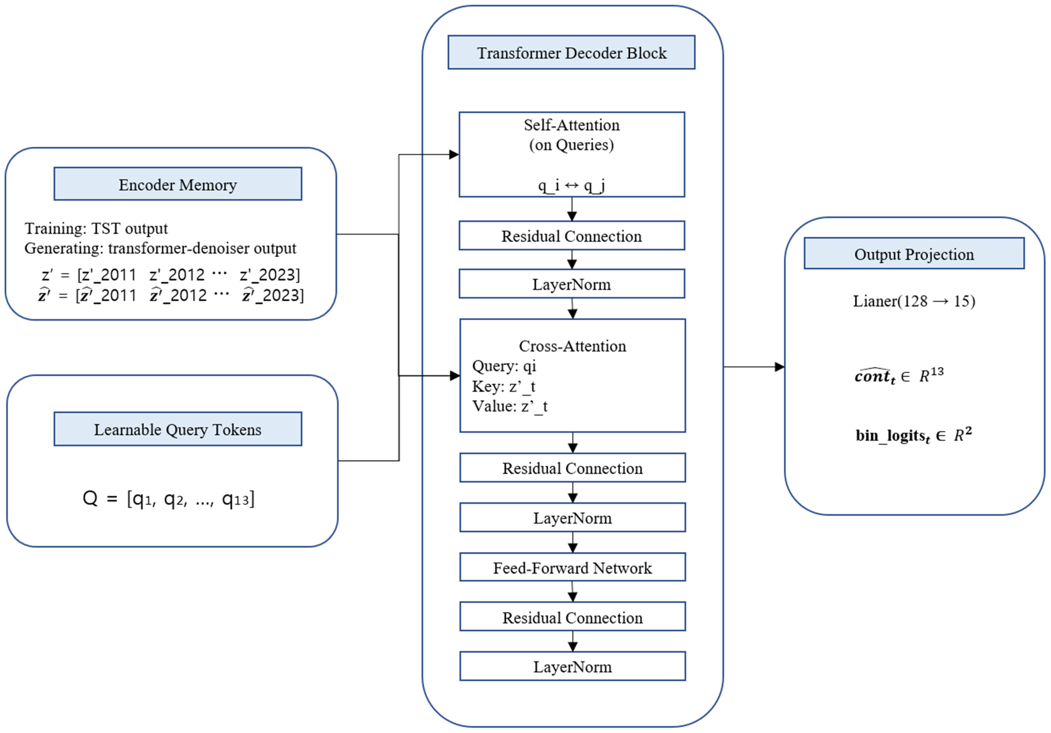
In our framework, we employ a TST-based Cross-Decoder to reconstruct year-level financial variables from the latent time series. The Cross-Decoder takes a sequence of learnable query tokens as input and uses a cross-attention mechanism that attends to the latent time series obtained via reverse diffusion as the encoder memory [38]. This design allows the model to stably recover financial variables corresponding to each year while preserving the temporal structure embedded in the latent representations.

3.6.1. Cross-Attention Decoder Architecture

Specifically, the decoder takes as input a learnable query token sequence of length $T=13$, $Q=\left[q_1,q_2,\dots ,q_{13}\right]$ where each query token represents a single year. Within the Transformer decoder blocks, self-attention is first applied among the query tokens to learn inter-year dependencies [38]. Then, in the cross-attention stage, the query tokens attend to the latent time-series representations restored via reverse diffusion as the memory.

In this cross-attention mechanism, each query $q_{\tau }$ is designed to reference information from all time steps of the latent time series as key–value pairs. This enables the decoder to consider not only the target year but also the global time-series context when reconstructing the financial state of a specific year. Unlike independent year-by-year reconstruction, this structure allows the model to recover financial variables while reflecting long-term financial trends and inter-temporal interactions.

Each Transformer decoder block consists of self-attention, cross-attention, and a feed-forward network, with residual connections and layer normalization applied between sublayers [38]. As the query tokens pass through multiple decoder blocks, they are progressively refined into year-level representations that integrate latent time-series information.

3.6.2. Output Projection and Variable Reconstruction

The output of the Cross-Decoder is a sequence of hidden vectors corresponding to year-level financial variables. This output is projected into the original financial variable space through a final linear mapping, producing predictions for both continuous and binary variables simultaneously. Specifically, the continuous variables are predicted as a 13-dimensional real-valued vector, while the binary variables are output in logit form.

During training, the Cross-Decoder takes the latent time series recovered via reverse diffusion as input and is optimized to reconstruct the original firm–year financial variables $x_{n,\tau }$. For the continuous variables, we use the mean squared error (MSE), and for the binary variables, we use the BCEWithLogits loss. Because this reconstruction loss is combined with the denoiser’s noise prediction loss to form the final Stage 2 objective, the Transformer-denoiser and the Cross-Decoder are jointly trained in Stage 2 by minimizing the following objective [5,6]. Final loss of Stage 2 is defined as Equation (16).

$$\begin{gathered} {\mathcal{L}}_{Stage2}={\mathcal{L}}_{diff}\left(\theta \right)+{\lambda }_{rec}{\mathcal{L}}_{rec}\left(\theta ,\psi \right) \\ {\mathcal{L}}_{rec}\left(\theta ,\psi \right)=E_n\left[{\displaystyle \frac{1}{T}}\sum _{\tau =1}^T\left({\mathcal{L}}_{\mathrm{c}\mathrm{o}\mathrm{n}\mathrm{t}}+{{\lambda }_{bin}\mathcal{L}}_{bin}\right)\right] \end{gathered}$$

(16)

where ${\mathcal{L}}_{diff}$ is the denoiser’s noise prediction loss defined in Equation (15) (with diffusion step s), and ${\lambda }_{rec}$ controls the trade-off between diffusion learning and financial-variable reconstruction.

3.6.3. Financial Time-Series Generation

During generation, we first sample a latent time series using the trained conditional diffusion model and then transform it into the financial variable space using the Cross-Decoder. For continuous variables, the decoder outputs are used directly. For binary variables, we apply a sigmoid function and discretize the results using a threshold of 0.5 to obtain the final values.

Overall, the proposed generation pipeline consists of two steps: conditional diffusion-based sampling in the latent time-series space and reconstruction of financial variables via a cross-attention decoder [5,6,38]. With this design, the proposed model can generate firm-level long-term financial time series while maintaining structural consistency across years, and the generated data can be leveraged for downstream tasks such as financial forecasting, risk analysis, and data augmentation. Figure 6 schematically illustrates the Cross-Decoder architecture, which reconstructs financial variables via cross-attention between learnable query tokens and the latent time series.

3.7. Post-Processing and Assignment of Year and Firm Identifiers

This section describes the post-processing procedure used to assign year and firm identifiers to the synthetic financial time series generated by the proposed pipeline. In this study, year and firm identifiers are not variables generated by the model itself; rather, they are metadata assigned a posteriori to organize the generated financial variables into an interpretable and usable firm-level panel data format.

3.7.1. Assignment of Year Information

Year information is provided as a conditional index for each time step (t = 0, …, 12). In our dataset, we map t to calendar years 2011–2023 for reporting and downstream evaluation. The proposed generative model does not treat calendar year as a prediction target. Instead, year information is incorporated as a conditional signal representing temporal position. Specifically, the generation process in the latent time-series space is performed on sequences of a fixed length, where each timestep is distinguished by its relative position within the sequence (0, 1, …, 12). This positional information is explicitly encoded within the model via positional encoding and year embeddings, allowing the model to recognize the temporal ordering of each timestep in the sequence.

After the generation process is completed, actual calendar years are assigned to each timestep through a one-to-one post hoc mapping. In this study, each generated sequence consists of 13 timesteps, which are sequentially mapped to calendar years from 2011 to 2023. This assignment is performed independently of the model outputs and serves to attach real-world year labels while preserving the relative temporal structure learned by the model.

3.7.2. Assignment of Firm Identifiers

The firm identifier (stock_id) is not generated by the model. Instead, we use a firm ID only as a conditioning key to capture firm-level heterogeneity during latent diffusion sampling. Specifically, for each synthetic sequence, we sample a conditioning firm ID from the training split according to a predefined sampling rule, generate a 13-step latent trajectory conditioned on the sampled firm ID (and other metadata such as year index and firm age), and decode it into financial variables.

After generation, we discard the conditioning firm ID for indexing purposes and assign a new virtual firm ID to the generated sequence so that it is treated as an additional firm in the synthetic panel. The assigned virtual firm ID is used only for panel organization and is not used as an input condition to the generator. All yearly observations within a generated sequence share the same virtual firm ID, resulting in a firm–year panel indexed by (virtual_stock_id, year).

3.7.3. Final Synthetic Panel Construction

Through the above procedures, the generated data are ultimately organized into a firm-level long-term financial panel dataset. Each row corresponds to the financial observations of a specific firm in a specific year and includes both continuous financial variables and binary financial indicators. Because the synthetic data conform to the same structural format as the original dataset, they can be directly utilized—without additional preprocessing—for downstream applications such as financial forecasting, risk analysis, and data augmentation.

In summary, the proposed generation framework synthesizes financial time series using a conditional latent diffusion model, reconstructs financial variables via a Cross-Decoder, and assigns year and firm identifiers in a post-processing step, thereby producing interpretable and practically usable synthetic firm-level panel data.

4. Empirical Analysis

This section systematically evaluates the statistical validity and predictive utility of the synthetic financial data generated by the Latent Financial Time-Series Diffusion model, which simultaneously captures nonlinear inter-variable interactions and year-wise temporal dependencies. Our dataset is derived from annual accounting/tax-related financial disclosures, where variables for year τ are typically finalized and become available after the fiscal year ends. As a result, we separate two evaluation settings: a static setting that assesses contemporaneous cross-sectional relationships within the same year (useful for explaining firm-value differences at time τ), and a dynamic setting that evaluates a one-year-ahead forecasting protocol (τ → τ + 1) that better matches information availability and practical prediction use cases.

In detail, we first assess how faithfully the proposed model preserves key statistical properties of the original data, including marginal distributions, correlation structures, and temporal continuity. The same evaluation protocol is applied to synthetic data generated by recent state-of-the-art generative models, enabling a quantitative comparison that highlights the relative advantages and distinctive property-preservation capabilities of the proposed approach [36].

Next, to examine the practical usefulness of the synthetic data, we compare the performance of predictive models trained solely on the original data with those trained using augmented datasets that incorporate the generated synthetic samples. In particular, this study goes beyond assessing gains attributable to a simple increase in sample size and instead disentangles the respective contributions of recovered inter-variable relationships and learned temporal patterns. To this end, component-wise ablation studies are conducted, and predictive performance is reported under both static prediction settings (within the same year) and dynamic prediction settings (from the previous year to the subsequent year).

All evaluations are conducted under strictly controlled conditions to ensure fair comparison: the same preprocessing pipeline, the same data generation ratio, identical training–validation splits, the same predictive models and hyperparameters, and multiple random-seed repetitions are consistently applied throughout. This design allows us to clearly attribute observed performance improvements to the structural and temporal properties preserved in the synthetic data, rather than to differences in experimental configurations. In addition, to assess robustness against stochasticity and model choice, we repeat all downstream prediction empirical evaluations with multiple random seeds and report results as mean ± standard deviation. We further validate the conclusions using both XGBoost and LightGBM regressors under the same experimental protocol.

4.1. Static Prediction Model Design

In this experiment, a static prediction model is constructed to predict firm value (MB, TQ) for a given year using financial characteristics from the same year as input variables. This setup aims to examine the relationship between cross-sectional financial attributes at a specific point in time and contemporaneous firm-level differences, and to quantitatively analyze how factors such as financial structure, profitability, and growth jointly affect firms’ market valuation. This setting is consistent with the year-wise cross-sectional analysis perspective widely adopted in empirical financial research [36]. Note that this static setting is intended to evaluate contemporaneous cross-sectional associations between firm characteristics and firm value within a given year, rather than a real-time forecasting scenario.

The input variables consist of 13 financial features: OWN, FORN, SIZE, LEV, CUR, GRW, ROE, CFO, PPE, INVREC, ROA, BIG4, and LOSS. The output variables are MB and TQ, which represent firm market value and performance.

Model training is conducted using data from 2011 to 2022, while data from 2023 are reserved as the test set for evaluating predictive performance. Specifically, the model learns the relationship between financial characteristics and firm value over the 2011–2022 period during training, and in the evaluation stage, it predicts MB and TQ for the year 2023 based on the corresponding input features. This approach is analogous to the year-wise cross-sectional regression framework commonly employed in empirical finance studies.

The model is based on an XGBoost regressor [13], designed to capture nonlinear structural patterns in the data. XGBoost is a decision-tree-based ensemble boosting method that is well known for its strong predictive performance and effective control of overfitting, making it suitable for financial data prediction [12,13]. Accordingly, we adopt this tree-based model as a robust and commonly used baseline for tabular financial variables, enabling a stable and fair evaluation of data augmentation effects without the sensitivity of neural networks to architecture choices and extensive hyperparameter tuning. To reduce reliance on a single predictive model, we additionally evaluate the same static prediction setting using a LightGBM regressor. LightGBM is a widely used gradient-boosted decision tree method for tabular financial data and is configured with a comparable model capacity to XGBoost, while all other experimental conditions are kept identical [13,41]. The XGBoost regression model is configured with 800 trees, a learning rate of 0.05, a maximum tree depth of 5, a subsampling ratio of 0.8, and a column sampling ratio of 0.8. Model performance is evaluated using four metrics: Root Mean Squared Error (RMSE), Mean Absolute Error (MAE), R² (coefficient of determination), and Mean Absolute Percentage Error (MAPE), as defined in Equations (17)–(20). All static prediction empirical evaluations are repeated across multiple random seeds, and the reported results are summarized as mean ± standard deviation. The R² metric indicates the proportion of variance in the dependent variable explained by the predictive model, RMSE and MAE measure the absolute magnitude of prediction errors, and MAPE reflects the relative scale of the prediction error.

$$RMSE=\sqrt{{\displaystyle \frac{1}{n}}\sum _{i=1}^n{\left(y_i-{\widehat{y}}_i\right)}^2}$$

(17)

$$MAE={\displaystyle \frac{1}{n}}\sum _{i=1}^n\left|y_i-{\widehat{y}}_i\right|$$

(18)

$$R^2=1-{\displaystyle \frac{{\sum }_{i=1}^n{\left(y_i-{\widehat{y}}_i\right)}^2}{{\sum }_{i=1}^n{\left(y_i-\overline{y}\right)}^2}}$$

(19)

$$MAPE={\displaystyle \frac{1}{n}}\sum _{i=1}^n\left|{\displaystyle \frac{y_i-{\widehat{y}}_i}{y_i}}\right|$$

(20)

The datasets consist of the original data and synthetic data generated by LFTD and its ablation variants, which are designed to isolate the contribution of each module in the full framework. LFTD comprises three components—FT, TST, and a diffusion denoiser—and we therefore evaluate LFTD-Denoiser-Only, LFTD-FT_Denoiser, LFTD-TST_Denoiser, and the full model LFTD-FT_TST_Denoiser. All models are evaluated using the same set of input variables and an identical XGBoost regression architecture with the same hyperparameter settings. Based on the model that achieves the best overall performance across the four evaluation metrics, we then conduct additional comparisons against widely used data augmentation baselines, including CTGAN [22], DDPM [6], and VAE-based models [5]. This stepwise evaluation design provides a consistent benchmark for analyzing how different generation and refinement strategies influence downstream predictive performance and reliability, thereby enabling a systematic assessment of the impact of synthetic data quality on the target prediction tasks.

4.2. Dynamic Prediction Model Design

In this evaluation setting, a dynamic prediction model is designed to predict firm value (MB, TQ) in the following year using financial characteristics from the previous year as input variables. This approach aims to quantitatively analyze how firm-level financial information accumulates over time and how its temporal evolution affects future market valuation. This dynamic protocol reflects the practical constraint that annual accounting/tax-related variables for year τ become usable for prediction only after the reporting cycle, making τ → τ + 1 a more realistic forecasting setup. In other words, to avoid information leakage, the generative model is trained using only the training period of each prediction setting, and synthetic samples are generated and used only within the corresponding training split.

For each firm, the data are sorted chronologically and restructured such that the input features from a given year $\tau$ are matched with the firm value in the subsequent year $\tau +1$. Specifically, financial characteristics from 2021 are used to predict firm value in 2022, and those from 2022 are used to predict firm value in 2023. This design captures time-lagged effects and enables a realistic assessment of how financial performance influences market valuation in subsequent periods.

Model training is conducted using data from 2011 to 2021, while the 2022 data are used as inputs to predict firm value in 2023. This temporally ordered training–evaluation split prevents data leakage and ensures that the model is validated under conditions that closely resemble real-world forecasting scenarios.

The model is based on an XGBoost regressor [13], which is designed to learn nonlinear structural patterns in the data. The XGBoost regression model is configured with 800 trees, a learning rate of 0.05, a maximum depth of 5, a subsampling ratio of 0.8, and a column sampling ratio of 0.8. As in the static prediction setting, the dynamic prediction setting is also evaluated using a LightGBM regressor to confirm that the results are not sensitive to the choice of predictive model [41].

Model performance is evaluated using four metrics: Root Mean Squared Error (RMSE), Mean Absolute Error (MAE), R² (coefficient of determination), and Mean Absolute Percentage Error (MAPE), as defined in Equations (17)–(20). All dynamic prediction results reported in this section are likewise averaged over multiple random seeds and presented as mean ± standard deviation.

4.3. Comparison and Analysis of Predictive Performance

This section provides a comprehensive analysis of the predictive performance of the proposed models and baseline methods under both static prediction (same-year prediction) and dynamic prediction (previous year → subsequent year) settings. Table 2 reports the performance of the proposed denoising-based models in the static prediction setting, while Table 3 presents the results in the dynamic prediction setting. In addition, Table 4 (static) and Table 5 (dynamic) compare the LFTD with conventional generative data augmentation methods, including DDPM, VAE, and CTGAN. Additional robustness results using LightGBM are provided in Table 6, Table 7, Table 8 and Table 9.

4.3.1. Static Prediction Performance Analysis

In the static prediction setting, LFTD achieves the best performance across all evaluation metrics.

For MB prediction (Table 2), LFTD records an RMSE of 0.282 and an R² of 0.949, substantially reducing prediction error and markedly improving explanatory power compared to the original data (RMSE 1.477, R² 0.206).

Similarly, for TQ prediction (Table 2), LFTD attains an RMSE of 0.170 and an R² of 0.955, demonstrating the highest predictive accuracy and explanatory power among all compared models.

While LFTD-FT+Denoiser achieves the lowest absolute error for MB prediction (RMSE 0.271), its R² value (0.857) is lower than that of LFTD. This indicates that although LFTD-FT+Denoiser effectively captures nonlinear inter-variable relationships, its inability to explicitly model temporal structure limits its overall explanatory power.

The LFTD-Denoiser model also yields relatively low RMSE values (MB 0.324, TQ 0.190); however, its R² scores (0.909 and 0.917, respectively) remain consistently below those of LFTD.

In contrast, LFTD-TST_Denoiser, which focuses solely on temporal structure, exhibits a substantial degradation in performance: for MB prediction, RMSE is 1.023 with an R² of 0.535, and for TQ prediction, RMSE is 0.593 with an R² of 0.522. These results suggest that while temporal continuity is preserved, the lack of sufficient modeling of nonlinear inter-variable interactions leads to significant information loss.

4.3.2. Dynamic Prediction Performance Analysis

A similar pattern is observed in the dynamic prediction setting (Table 3). LFTD consistently delivers the most stable and superior performance, achieving an RMSE of 0.304 and an R² of 0.940 for MB prediction, and an RMSE of 0.182 with an R² of 0.949 for TQ prediction. This demonstrates the model’s effectiveness in capturing time-lagged structures and cumulative effects when predicting firm value in the subsequent year based on prior-year financial information.

Both LFTD-FT+Denoiser and LFTD-Denoiser maintain relatively low RMSE values in the dynamic setting; however, their explanatory power remains lower than that of LFTD, with R² values of 0.843 and 0.902, respectively, for MB prediction.

The performance of LFTD-TST_Denoiser further deteriorates in the dynamic setting, with MB prediction results of RMSE 1.114 and R² 0.449, and TQ prediction results of RMSE 0.598 and R² 0.515. These findings indicate that temporal information alone is insufficient to adequately explain inter-year variations in firm value.

4.3.3. Comparison with Conventional Generative Data Augmentation Methods

Using LFTD as the benchmark, comparative results with traditional data augmentation methods are presented in Table 4 (static) and Table 5 (dynamic).

In the static prediction setting, DDPM exhibits moderate explanatory power, with R² values of 0.524 for MB and 0.679 for TQ; however, its RMSE values are considerably high (1.896 and 1.126, respectively).

VAE demonstrates relatively stable performance (MB: RMSE 0.745, R² 0.377; TQ: RMSE 0.462, R² 0.410), though its explanatory power remains limited.

CTGAN performs poorly even in the static setting, with low R² values (MB 0.231, TQ 0.305), indicating an inability to adequately learn the structural properties of financial data.

These limitations become more pronounced in the dynamic prediction setting. Both DDPM and CTGAN exhibit R² values that drop to zero or become negative for both MB and TQ, reflecting a severe loss of predictive stability. VAE likewise shows minimal explanatory power, with R² values remaining around 0.004. These results suggest that probabilistic generative models fail to preserve temporal dependencies and structural continuity across years.

In contrast, LFTD consistently achieves the highest R² values and maintains stable error levels across both static and dynamic settings. This performance underscores the advantage of a refinement- and reconstruction-centered approach, which jointly captures nonlinear structural relationships and cumulative temporal effects inherent in financial data. Overall, LFTD is shown to overcome the variance inflation and instability issues commonly encountered by conventional generative augmentation methods, while simultaneously improving prediction accuracy and generalization performance in firm value forecasting.

Table 2. MB, TQ static prediction performance of proposed denoising-based models using XGBoost.

	MB Prediction Performance Comparison				TQ Prediction Performance Comparison
DataSet	RMSE	MAE	R2	MAPE	RMSE	MAE	R2	MAPE
Original	1.477 ± 0.012	0.844 ± 0.005	0.206 ± 0.013	0.882 ± 0.006	0.866 ± 0.004	0.500 ± 0.003	0.236 ± 0.007	0.462 ± 0.003
LFTD	0.282 ± <0.001	0.109 ± <0.001	0.949 ± <0.001	0.106 ± 0.001	0.170 ± <0.001	0.065 ± <0.001	0.955 ± <0.001	0.057 ± <0.001
LFTD-TST_Denoiser	1.023 ± 0.001	0.551 ± <0.001	0.535 ± 0.001	0.440 ± 0.001	0.593 ± <0.001	0.324 ± <0.001	0.522 ± <0.001	0.265 ± <0.001
LFTD-FT_Denoiser	0.271 ± <0.001	0.110 ± <0.001	0.857 ± <0.001	0.078 ± <0.001	0.163 ± <0.001	0.069 ± <0.001	0.856 ± 0.001	0.052 ± <0.001
LFTD-Denoiser-Only	0.324 ± <0.001	0.183 ± <0.001	0.909 ± <0.001	0.131 ± <0.001	0.190 ± <0.001	0.105 ± <0.001	0.917 ± <0.001	0.078 ± <0.001

Table 2. MB, TQ static prediction performance of proposed denoising-based models using XGBoost.

	MB Prediction Performance Comparison				TQ Prediction Performance Comparison
DataSet	RMSE	MAE	R2	MAPE	RMSE	MAE	R2	MAPE
Original	1.477 ± 0.012	0.844 ± 0.005	0.206 ± 0.013	0.882 ± 0.006	0.866 ± 0.004	0.500 ± 0.003	0.236 ± 0.007	0.462 ± 0.003
LFTD	0.282 ± <0.001	0.109 ± <0.001	0.949 ± <0.001	0.106 ± 0.001	0.170 ± <0.001	0.065 ± <0.001	0.955 ± <0.001	0.057 ± <0.001
LFTD-TST_Denoiser	1.023 ± 0.001	0.551 ± <0.001	0.535 ± 0.001	0.440 ± 0.001	0.593 ± <0.001	0.324 ± <0.001	0.522 ± <0.001	0.265 ± <0.001
LFTD-FT_Denoiser	0.271 ± <0.001	0.110 ± <0.001	0.857 ± <0.001	0.078 ± <0.001	0.163 ± <0.001	0.069 ± <0.001	0.856 ± 0.001	0.052 ± <0.001
LFTD-Denoiser-Only	0.324 ± <0.001	0.183 ± <0.001	0.909 ± <0.001	0.131 ± <0.001	0.190 ± <0.001	0.105 ± <0.001	0.917 ± <0.001	0.078 ± <0.001

Table 3. MB, TQ forecasting of proposed denoising-based models using previous-year features using XGBoost.

	MB Prediction Performance Comparison				TQ Prediction Performance Comparison
DataSet	RMSE	MAE	R2	MAPE	RMSE	MAE	R2	MAPE
Original	1.519 ± 0.004	0.877 ± 0.004	0.161 ± 0.004	0.935 ± 0.003	0.892 ± 0.003	0.521 ± 0.003	0.189 ± 0.005	0.486 ± 0.003
LFTD	0.304 ± <0.001	0.113 ± <0.001	0.940 ± <0.001	0.112 ± <0.001	0.182 ± <0.001	0.068 ± <0.001	0.949 ± <0.001	0.060 ± <0.001
LFTD-TST_Denoiser	1.114 ± <0.001	0.580 ± <0.001	0.449 ± <0.001	0.456 ± <0.001	0.598 ± <0.001	0.328 ± <0.001	0.515 ± 0.001	0.273 ± <0.001
LFTD-FT_Denoiser	0.284 ± 0.001	0.112 ± <0.001	0.843 ± 0.001	0.080 ± <0.001	0.169 ± <0.001	0.070 ± <0.001	0.846 ± <0.001	0.053 ± <0.001
LFTD-Denoiser-Only	0.336 ± 0.001	0.185 ± <0.001	0.902 ± <0.001	0.135 ± <0.001	0.196 ± <0.001	0.106 ± <0.001	0.912 ± <0.001	0.080 ± <0.001

Table 3. MB, TQ forecasting of proposed denoising-based models using previous-year features using XGBoost.

	MB Prediction Performance Comparison				TQ Prediction Performance Comparison
DataSet	RMSE	MAE	R2	MAPE	RMSE	MAE	R2	MAPE
Original	1.519 ± 0.004	0.877 ± 0.004	0.161 ± 0.004	0.935 ± 0.003	0.892 ± 0.003	0.521 ± 0.003	0.189 ± 0.005	0.486 ± 0.003
LFTD	0.304 ± <0.001	0.113 ± <0.001	0.940 ± <0.001	0.112 ± <0.001	0.182 ± <0.001	0.068 ± <0.001	0.949 ± <0.001	0.060 ± <0.001
LFTD-TST_Denoiser	1.114 ± <0.001	0.580 ± <0.001	0.449 ± <0.001	0.456 ± <0.001	0.598 ± <0.001	0.328 ± <0.001	0.515 ± 0.001	0.273 ± <0.001
LFTD-FT_Denoiser	0.284 ± 0.001	0.112 ± <0.001	0.843 ± 0.001	0.080 ± <0.001	0.169 ± <0.001	0.070 ± <0.001	0.846 ± <0.001	0.053 ± <0.001
LFTD-Denoiser-Only	0.336 ± 0.001	0.185 ± <0.001	0.902 ± <0.001	0.135 ± <0.001	0.196 ± <0.001	0.106 ± <0.001	0.912 ± <0.001	0.080 ± <0.001

Table 4. MB, TQ static prediction performance comparison between proposed and conventional augmentation models using XGBoost.

	MB Prediction Performance Comparison				TQ Prediction Performance Comparison
DataSet	RMSE	MAE	R2	MAPE	RMSE	MAE	R2	MAPE
Original	1.477 ± 0.012	0.844 ± 0.005	0.206 ± 0.013	0.882 ± 0.006	0.866 ± 0.004	0.500 ± 0.003	0.236 ± 0.007	0.462 ± 0.003
LFTD	0.282 ± <0.001	0.109 ± <0.001	0.949 ± <0.001	0.106 ± 0.001	0.170 ± <0.001	0.065 ± <0.001	0.955 ± <0.001	0.057 ± <0.001
DDPM	1.896 ± <0.001	1.050 ± <0.001	0.524 ± <0.001	1.146 ± <0.001	1.126 ± <0.001	0.627 ± <0.001	0.679 ± <0.001	0.511 ± <0.001
VAE	0.745 ± <0.001	0.514 ± <0.001	0.377 ± <0.001	0.400 ± <0.001	0.462 ± <0.001	0.315 ± <0.001	0.410 ± <0.001	0.250 ± <0.001
CTGAN	1.387 ± <0.001	0.821 ± <0.001	0.231 ± <0.001	0.574 ± <0.001	0.987 ± <0.001	0.551 ± <0.001	0.305 ± <0.001	0.374 ± <0.001

Table 4. MB, TQ static prediction performance comparison between proposed and conventional augmentation models using XGBoost.

	MB Prediction Performance Comparison				TQ Prediction Performance Comparison
DataSet	RMSE	MAE	R2	MAPE	RMSE	MAE	R2	MAPE
Original	1.477 ± 0.012	0.844 ± 0.005	0.206 ± 0.013	0.882 ± 0.006	0.866 ± 0.004	0.500 ± 0.003	0.236 ± 0.007	0.462 ± 0.003
LFTD	0.282 ± <0.001	0.109 ± <0.001	0.949 ± <0.001	0.106 ± 0.001	0.170 ± <0.001	0.065 ± <0.001	0.955 ± <0.001	0.057 ± <0.001
DDPM	1.896 ± <0.001	1.050 ± <0.001	0.524 ± <0.001	1.146 ± <0.001	1.126 ± <0.001	0.627 ± <0.001	0.679 ± <0.001	0.511 ± <0.001
VAE	0.745 ± <0.001	0.514 ± <0.001	0.377 ± <0.001	0.400 ± <0.001	0.462 ± <0.001	0.315 ± <0.001	0.410 ± <0.001	0.250 ± <0.001
CTGAN	1.387 ± <0.001	0.821 ± <0.001	0.231 ± <0.001	0.574 ± <0.001	0.987 ± <0.001	0.551 ± <0.001	0.305 ± <0.001	0.374 ± <0.001

Table 5. MB, TQ forecasting of generative augmentation models using previous-year features using XGBoost.

	MB Prediction Performance Comparison				TQ Prediction Performance Comparison
DataSet	RMSE	MAE	R2	MAPE	RMSE	MAE	R2	MAPE
Original	1.519 ± 0.004	0.877 ± 0.004	0.161 ± 0.004	0.935 ± 0.003	0.892 ± 0.003	0.521 ± 0.003	0.189 ± 0.005	0.486 ± 0.003
LFTD	0.304 ± <0.001	0.113 ± <0.001	0.940 ± <0.001	0.112 ± <0.001	0.182 ± <0.001	0.068 ± <0.001	0.949 ± <0.001	0.060 ± <0.001
DDPM	2.751 ± <0.001	1.621 ± <0.001	−0.002 ± <0.001	1.684 ± <0.001	1.991 ± <0.001	1.279 ± <0.001	−0.002 ± <0.001	0.928 ± <0.001
VAE	0.942 ± <0.001	0.701 ± <0.001	0.003 ± <0.001	0.581 ± <0.001	0.601 ± <0.001	0.442 ± <0.001	0.004 ± <0.001	0.366 ± <0.001
CTGAN	1.583 ± <0.001	1.039 ± <0.001	−0.002 ± <0.001	0.831 ± <0.001	1.185 ± <0.001	0.785 ± <0.001	−0.002 ± <0.001	0.605 ± <0.001

Table 5. MB, TQ forecasting of generative augmentation models using previous-year features using XGBoost.

	MB Prediction Performance Comparison				TQ Prediction Performance Comparison
DataSet	RMSE	MAE	R2	MAPE	RMSE	MAE	R2	MAPE
Original	1.519 ± 0.004	0.877 ± 0.004	0.161 ± 0.004	0.935 ± 0.003	0.892 ± 0.003	0.521 ± 0.003	0.189 ± 0.005	0.486 ± 0.003
LFTD	0.304 ± <0.001	0.113 ± <0.001	0.940 ± <0.001	0.112 ± <0.001	0.182 ± <0.001	0.068 ± <0.001	0.949 ± <0.001	0.060 ± <0.001
DDPM	2.751 ± <0.001	1.621 ± <0.001	−0.002 ± <0.001	1.684 ± <0.001	1.991 ± <0.001	1.279 ± <0.001	−0.002 ± <0.001	0.928 ± <0.001
VAE	0.942 ± <0.001	0.701 ± <0.001	0.003 ± <0.001	0.581 ± <0.001	0.601 ± <0.001	0.442 ± <0.001	0.004 ± <0.001	0.366 ± <0.001
CTGAN	1.583 ± <0.001	1.039 ± <0.001	−0.002 ± <0.001	0.831 ± <0.001	1.185 ± <0.001	0.785 ± <0.001	−0.002 ± <0.001	0.605 ± <0.001

Table 6. MB, TQ static prediction performance of proposed denoising-based models using LightGBM.

	MB Prediction Performance Comparison				TQ Prediction Performance Comparison
DataSet	RMSE	MAE	R2	MAPE	RMSE	MAE	R2	MAPE
Original	1.475 ± 0.005	0.838 ± 0.003	0.208 ± 0.005	0.865 ± 0.005	0.869 ± 0.003	0.502 ± 0.002	0.232 ± 0.005	0.461 ± 0.002
LFTD	0.269 ± 0.001	0.106 ± <0.001	0.953 ± <0.001	0.106 ± <0.001	0.162 ± 0.001	0.064 ± <0.001	0.959 ± 0.001	0.057 ± <0.001
LFTD-TST_Denoiser	1.004 ± <0.001	0.542 ± <0.001	0.552 ± <0.001	0.436 ± <0.001	0.585 ± <0.001	0.320 ± <0.001	0.535 ± 0.001	0.264 ± <0.001
LFTD-FT_Denoiser	0.267 ± <0.001	0.109 ± <0.001	0.861 ± <0.001	0.078 ± <0.001	0.160 ± <0.001	0.067 ± <0.001	0.862 ± 0.001	0.052 ± <0.001
LFTD-Denoiser-Only	0.316 ± <0.001	0.179 ± <0.001	0.913 ± <0.001	0.131 ± <0.001	0.186 ± <0.001	0.104 ± <0.001	0.920 ± <0.001	0.078 ± <0.001

Table 6. MB, TQ static prediction performance of proposed denoising-based models using LightGBM.

	MB Prediction Performance Comparison				TQ Prediction Performance Comparison
DataSet	RMSE	MAE	R2	MAPE	RMSE	MAE	R2	MAPE
Original	1.475 ± 0.005	0.838 ± 0.003	0.208 ± 0.005	0.865 ± 0.005	0.869 ± 0.003	0.502 ± 0.002	0.232 ± 0.005	0.461 ± 0.002
LFTD	0.269 ± 0.001	0.106 ± <0.001	0.953 ± <0.001	0.106 ± <0.001	0.162 ± 0.001	0.064 ± <0.001	0.959 ± 0.001	0.057 ± <0.001
LFTD-TST_Denoiser	1.004 ± <0.001	0.542 ± <0.001	0.552 ± <0.001	0.436 ± <0.001	0.585 ± <0.001	0.320 ± <0.001	0.535 ± 0.001	0.264 ± <0.001
LFTD-FT_Denoiser	0.267 ± <0.001	0.109 ± <0.001	0.861 ± <0.001	0.078 ± <0.001	0.160 ± <0.001	0.067 ± <0.001	0.862 ± 0.001	0.052 ± <0.001
LFTD-Denoiser-Only	0.316 ± <0.001	0.179 ± <0.001	0.913 ± <0.001	0.131 ± <0.001	0.186 ± <0.001	0.104 ± <0.001	0.920 ± <0.001	0.078 ± <0.001

Table 7. MB, TQ forecasting of proposed denoising-based models using previous-year features using LightGBM.

	MB Prediction Performance Comparison				TQ Prediction Performance Comparison
DataSet	RMSE	MAE	R2	MAPE	RMSE	MAE	R2	MAPE
Original	1.505 ± 0.002	0.870 ± 0.002	0.176 ± 0.002	0.947 ± 0.002	0.886 ± 0.003	0.518 ± 0.002	0.201 ± 0.005	0.489 ± 0.002
LFTD	0.309 ± <0.001	0.125 ± <0.001	0.938 ± <0.001	0.132 ± <0.001	0.185 ± <0.001	0.075 ± <0.001	0.947 ± <0.001	0.069 ± <0.001
LFTD-TST_Denoiser	1.126 ± <0.001	0.579 ± <0.001	0.438 ± <0.001	0.456 ± <0.001	0.603 ± <0.001	0.328 ± <0.001	0.505 ± <0.001	0.274 ± <0.001
LFTD-FT_Denoiser	0.293 ± <0.001	0.130 ± <0.001	0.833 ± <0.001	0.092 ± <0.001	0.175 ± <0.001	0.080 ± <0.001	0.835 ± <0.001	0.062 ± <0.001
LFTD-Denoiser-Only	0.354 ± <0.001	0.205 ± <0.001	0.891 ± <0.001	0.154 ± <0.001	0.205 ± <0.001	0.115 ± <0.001	0.904 ± <0.001	0.089 ± <0.001

Table 7. MB, TQ forecasting of proposed denoising-based models using previous-year features using LightGBM.

	MB Prediction Performance Comparison				TQ Prediction Performance Comparison
DataSet	RMSE	MAE	R2	MAPE	RMSE	MAE	R2	MAPE
Original	1.505 ± 0.002	0.870 ± 0.002	0.176 ± 0.002	0.947 ± 0.002	0.886 ± 0.003	0.518 ± 0.002	0.201 ± 0.005	0.489 ± 0.002
LFTD	0.309 ± <0.001	0.125 ± <0.001	0.938 ± <0.001	0.132 ± <0.001	0.185 ± <0.001	0.075 ± <0.001	0.947 ± <0.001	0.069 ± <0.001
LFTD-TST_Denoiser	1.126 ± <0.001	0.579 ± <0.001	0.438 ± <0.001	0.456 ± <0.001	0.603 ± <0.001	0.328 ± <0.001	0.505 ± <0.001	0.274 ± <0.001
LFTD-FT_Denoiser	0.293 ± <0.001	0.130 ± <0.001	0.833 ± <0.001	0.092 ± <0.001	0.175 ± <0.001	0.080 ± <0.001	0.835 ± <0.001	0.062 ± <0.001
LFTD-Denoiser-Only	0.354 ± <0.001	0.205 ± <0.001	0.891 ± <0.001	0.154 ± <0.001	0.205 ± <0.001	0.115 ± <0.001	0.904 ± <0.001	0.089 ± <0.001

Table 8. MB, TQ static prediction performance comparison between proposed and conventional augmentation models using LightGBM.

	MB Prediction Performance Comparison				TQ Prediction Performance Comparison
DataSet	RMSE	MAE	R2	MAPE	RMSE	MAE	R2	MAPE
Original	1.475 ± 0.005	0.838 ± 0.003	0.208 ± 0.005	0.865 ± 0.005	0.869 ± 0.003	0.502 ± 0.002	0.232 ± 0.005	0.461 ± 0.002
LFTD	0.269 ± 0.001	0.106 ± <0.001	0.953 ± <0.001	0.106 ± <0.001	0.162 ± 0.001	0.064 ± <0.001	0.959 ± <0.001	0.057 ± <0.001
DDPM	1.879 ± <0.001	1.038 ± <0.001	0.532 ± <0.001	1.124 ± <0.001	1.122 ± <0.001	0.624 ± <0.001	0.682 ± <0.001	0.509 ± <0.001
VAE	0.742 ± <0.001	0.512 ± <0.001	0.382 ± <0.001	0.398 ± <0.001	0.461 ± <0.001	0.314 ± <0.001	0.414 ± <0.001	0.249 ± <0.001
CTGAN	1.386 ± <0.001	0.820 ± <0.001	0.231 ± <0.001	0.574 ± <0.001	0.987 ± <0.001	0.551 ± <0.001	0.305 ± <0.001	0.374 ± <0.001

Table 8. MB, TQ static prediction performance comparison between proposed and conventional augmentation models using LightGBM.

	MB Prediction Performance Comparison				TQ Prediction Performance Comparison
DataSet	RMSE	MAE	R2	MAPE	RMSE	MAE	R2	MAPE
Original	1.475 ± 0.005	0.838 ± 0.003	0.208 ± 0.005	0.865 ± 0.005	0.869 ± 0.003	0.502 ± 0.002	0.232 ± 0.005	0.461 ± 0.002
LFTD	0.269 ± 0.001	0.106 ± <0.001	0.953 ± <0.001	0.106 ± <0.001	0.162 ± 0.001	0.064 ± <0.001	0.959 ± <0.001	0.057 ± <0.001
DDPM	1.879 ± <0.001	1.038 ± <0.001	0.532 ± <0.001	1.124 ± <0.001	1.122 ± <0.001	0.624 ± <0.001	0.682 ± <0.001	0.509 ± <0.001
VAE	0.742 ± <0.001	0.512 ± <0.001	0.382 ± <0.001	0.398 ± <0.001	0.461 ± <0.001	0.314 ± <0.001	0.414 ± <0.001	0.249 ± <0.001
CTGAN	1.386 ± <0.001	0.820 ± <0.001	0.231 ± <0.001	0.574 ± <0.001	0.987 ± <0.001	0.551 ± <0.001	0.305 ± <0.001	0.374 ± <0.001

Table 9. MB, TQ forecasting of generative augmentation models using previous-year features using LightGBM.

	MB Prediction Performance Comparison				TQ Prediction Performance Comparison
DataSet	RMSE	MAE	R2	MAPE	RMSE	MAE	R2	MAPE
Original	1.505 ± 0.002	0.870 ± 0.002	0.176 ± 0.002	0.947 ± 0.002	0.886 ± 0.003	0.518 ± 0.002	0.201 ± 0.005	0.489 ± 0.002
LFTD	0.309 ± <0.001	0.125 ± <0.001	0.938 ± <0.001	0.132 ± <0.001	0.185 ± <0.001	0.075 ± <0.001	0.947 ± <0.001	0.069 ± <0.001
DDPM	2.748 ± <0.001	1.619 ± <0.001	−0.000 ± <0.001	1.683 ± <0.001	1.989 ± <0.001	1.278 ± <0.001	−0.000 ± <0.001	0.927 ± <0.001
VAE	0.941 ± <0.001	0.701 ± <0.001	0.005 ± <0.001	0.581 ± <0.001	0.600 ± <0.001	0.441 ± <0.001	0.005 ± <0.001	0.366 ± <0.001
CTGAN	1.581 ± <0.001	1.038 ± <0.001	−0.000 ± <0.001	0.831 ± <0.001	1.184 ± <0.001	0.784 ± <0.001	−0.000 ± <0.001	0.604 ± <0.001

Table 9. MB, TQ forecasting of generative augmentation models using previous-year features using LightGBM.

	MB Prediction Performance Comparison				TQ Prediction Performance Comparison
DataSet	RMSE	MAE	R2	MAPE	RMSE	MAE	R2	MAPE
Original	1.505 ± 0.002	0.870 ± 0.002	0.176 ± 0.002	0.947 ± 0.002	0.886 ± 0.003	0.518 ± 0.002	0.201 ± 0.005	0.489 ± 0.002
LFTD	0.309 ± <0.001	0.125 ± <0.001	0.938 ± <0.001	0.132 ± <0.001	0.185 ± <0.001	0.075 ± <0.001	0.947 ± <0.001	0.069 ± <0.001
DDPM	2.748 ± <0.001	1.619 ± <0.001	−0.000 ± <0.001	1.683 ± <0.001	1.989 ± <0.001	1.278 ± <0.001	−0.000 ± <0.001	0.927 ± <0.001
VAE	0.941 ± <0.001	0.701 ± <0.001	0.005 ± <0.001	0.581 ± <0.001	0.600 ± <0.001	0.441 ± <0.001	0.005 ± <0.001	0.366 ± <0.001
CTGAN	1.581 ± <0.001	1.038 ± <0.001	−0.000 ± <0.001	0.831 ± <0.001	1.184 ± <0.001	0.784 ± <0.001	−0.000 ± <0.001	0.604 ± <0.001

5. Conclusions

This paper has proposed LFTD, a generative framework for producing synthetic firm-level financial data that preserves both the tabular and time-series structures of financial statements. Rather than simply generating “plausible-looking” values, the framework is designed to respect accounting constraints, inter-variable dependencies, and temporal evolution. The proposed approach consists of three main stages. First, annual financial statements are embedded to obtain compact representations of firms’ financial conditions. Second, temporal patterns are learned to capture long-term dynamics at the firm level. Finally, a diffusion-based conditional generation process uses these representations to reconstruct and generate new financial time series that satisfy financial consistency and temporal coherence. In this way, the method reflects the hybrid tabular–time-series structure and strong accounting restrictions inherent in financial data. Experimental results show that the data generated by LFTD preserve statistically meaningful structures, consistently reproducing the qualitative relationships between financial indicators and firm value observed in the original data. Moreover, when these synthetic data are used as additional training samples for downstream prediction models, they improve model performance in both static and dynamic prediction settings. In particular, they enhance explanatory power and generalization while maintaining comparable error levels. These findings suggest that structure-aware, diffusion-based augmentation can serve as a practical tool for boosting model performance in financial data analysis.