Article

A Deep Reinforcement Learning Framework for Strategic Indian NIFTY 50 Index Trading

1
School of Technology Management and Engineering (STME), SVKM’s NMIMS Deemed to be University, Indore 453112, India
2
Symbiosis Institute of Technology, Symbiosis International (Deemed University) (SIU), Pune 412115, India
3
School of Computer Science Engineering & Applications, D. Y. Patil International University (DYPIU), Pune 411044, India
*
Authors to whom correspondence should be addressed.
AI 2025, 6(8), 183; https://doi.org/10.3390/ai6080183
Submission received: 9 July 2025 / Revised: 7 August 2025 / Accepted: 8 August 2025 / Published: 11 August 2025
(This article belongs to the Special Issue AI in Finance: Leveraging AI to Transform Financial Services)

Abstract

This paper presents a comprehensive deep reinforcement learning (DRL) framework for developing strategic trading models tailored to the Indian NIFTY 50 index, leveraging the temporal and nonlinear nature of financial markets. Three advanced DRL architectures deep Q-network (DQN), double deep Q-network (DDQN), and dueling double deep Q-network (Dueling DDQN) were implemented and empirically evaluated. Using a decade-long dataset of 15-min interval OHLC data enriched with technical indicators such as the exponential moving average (EMA), pivot points, and multiple supertrend configurations, the models were trained using prioritized experience replay, epsilon-greedy exploration strategies, and softmax sampling mechanisms. A test set comprising one year of unseen data (May 2024–April 2025) was used to assess generalization performance across key financial metrics, including Sharpe ratio, profit factor, win rate, and trade frequency. Each architecture was analyzed in three progressively sophisticated variants incorporating enhancements in reward shaping, exploration–exploitation balancing, and penalty-based trade constraints. DDQN V3 achieved a Sharpe ratio of 0.7394, a 73.33% win rate, and a 16.58 profit factor across 15 trades, indicating strong volatility-adjusted suitability for real-world deployment. In contrast, the Dueling DDQN V3 achieved a high Sharpe ratio of 1.2278 and a 100% win rate but with only three trades, indicating an excessive conservatism. The DQN V1 model served as a strong baseline, outperforming passive strategies but exhibiting limitations due to Q-value overestimation. The novelty of this work lies in its systematic exploration of DRL variants integrated with enhanced exploration mechanisms and reward–penalty structures, rigorously applied to high-frequency trading on the NIFTY 50 index within an emerging market context. Our findings underscore the critical importance of architectural refinements, dynamic exploration strategies, and trade regularization in stabilizing learning and enhancing profitability in DRL-based intelligent trading systems.

1. Introduction

The Indian stock market has experienced remarkable growth in the past decade, driven by increased participation from both retail and institutional investors. Demat accounts surged from approximately 2.3 crore to over 22 crore, retail trading volumes now constitute about 45–50% of cash market turnover, and retail mutual fund AUM has grown eightfold alongside total MF AUM expanding more than sixfold [1]. This expansion has created a fertile landscape for the development of sophisticated automated trading strategies capable of navigating the complexities of an emerging financial market. At the forefront of this market is the NIFTY 50 index, which represents the top 50 companies listed on the National Stock Exchange (NSE) of India and serves as a key benchmark reflecting the overall health and performance of the Indian economy. Developing effective trading strategies for such an index not only presents significant commercial opportunities but also introduces complex challenges due to the dynamic, nonstationary, and noisy nature of financial time series data.
Traditional quantitative and machine learning-based trading methods have shown promising results in capturing patterns within historical market data [2,3]. However, these approaches often struggle to adapt in real time to evolving market conditions and intricate dependencies within asset price movements [3,4]. DRL, which synergizes the representation power of deep neural networks with the trial-and-error learning paradigm of reinforcement learning, has emerged as a powerful paradigm for sequential decision-making problems in complex and uncertain environments. By interacting directly with the market environment and continuously learning from feedback, DRL agents can develop autonomous trading policies that optimize long-term objectives, such as maximizing returns while controlling risk exposure.
While DRL has become popular in global equity and futures markets, its application to emerging markets such as India, especially using high-frequency data, remains limited. Furthermore, many existing studies rely on simulated environments or low-frequency datasets and do not report key performance metrics such as Sharpe ratio, drawdown, or win rate. This makes it difficult to assess the practical viability and robustness of DRL-based trading strategies in real-world financial contexts.
This paper focuses on applying DRL techniques to the NIFTY 50 index by investigating three prominent architectures: DQN, DDQN, and Dueling DDQN. These models address key challenges in reinforcement learning, including overestimation bias and inefficient value function approximation, thereby enabling more stable and effective learning of optimal trading strategies. Using a comprehensive dataset that spans nine years of historical price and volume data for training, combined with one year of unseen market data for validation and testing, the study aims to rigorously evaluate the performance and generalization capabilities of these models. The ultimate goal is to demonstrate that DRL-based frameworks can deliver robust and consistent buy and sell signals tailored to the unique characteristics of the Indian stock market, thus contributing to the growing body of research on intelligent trading systems in emerging markets.

2. Related Work

The DRL has emerged as a promising approach in financial market modeling due to its capacity to adapt in dynamic, partially observable environments. Several studies have explored variants of DRL for stock trading, portfolio optimization, and signal generation, though with varying levels of empirical rigor, market scope, and practical relevance.
Awad et al. [5] implemented a DQN-based trading agent on gold prices and reported performance improvements over LSTM and SVM models. However, the study was confined to a small dataset and did not evaluate risk-adjusted returns, limiting its generalizability. In contrast, Nuipian et al. [6] employed DQN for portfolio optimization on S&P 500 assets and achieved approximately 15% higher cumulative returns over traditional strategies, yet failed to report Sharpe ratios or drawdown, and did not simulate transaction costs, which are crucial for real-world applicability.
Du and Shen [7] proposed a sentiment-aware DRL model using BERT to integrate financial news with price data. While the hybrid approach showed promising returns on newly listed Chinese stocks, its effectiveness on established, high-volume markets remains untested. Similarly, Hossain et al. [8] incorporated fine-tuned technical indicators (MACD, RSI) into a DQN architecture but evaluated performance based on signal accuracy rather than actual trading profits or risk metrics.
Sagiraju and Mogalla [9] extended DRL frameworks by incorporating market sentiment heuristics but used manually tagged news and omitted key trading metrics, weakening the empirical support.
Several survey works [10,11] offer broader context: Mienye et al. [10] reviewed deep learning applications across finance but only briefly mentioned DRL, while Hu et al. [11] focused on deep learning for price prediction and acknowledged the limited application of reinforcement learning in practice.
Hiransha et al. [12] benchmarked deep learning models like LSTM and CNN for NSE price prediction. Though LSTM outperformed others in directional accuracy, the work did not evaluate trading strategy performance or risk-adjusted profitability. Yang et al. [13] presented a more sophisticated ensemble strategy combining PPO, A2C, and DDPG. Tested on the Dow 30 stocks, their approach showed improved cumulative returns and lower volatility compared to individual agents, thus highlighting the value of ensemble learning in DRL.
Zhang et al. [14] tested DRL models on a large-scale futures dataset (2011–2019) with volatility-adjusted reward functions. The approach outperformed momentum baselines even after accounting for transaction costs, offering credible evidence of DRL’s robustness in diverse asset classes. Singh et al. [15] provided a conceptual review of DRL’s use in financial decision-making, calling attention to practical deployment challenges like explainability and adaptivity but lacking model-specific performance evaluations.
Kabbani and Duman [16] modeled stock trading as a partially observable Markov decision process (POMDP), enabling real-time trade automation. While the method showed profit potential in the Turkish market, results lacked standard benchmarks or comparative evaluation. Théate and Ernst [17] introduced the trading deep Q-network (TDQN), which directly optimizes Sharpe ratio on synthetic trajectories. While the reward engineering is innovative, reliance on simulated data raises concerns about overfitting and realism.
Li et al. [18] proposed a robust DRL architecture for noisy market conditions. Their method outperformed standard DQN in volatile environments, although it was tested only on Chinese equities and lacked cross-asset or cross-market evaluations.
Cheng et al. [19] emphasized interpretability in their DRL-based trading framework and outperformed basic technical strategies on Taiwanese data. However, their evaluation relied on ROI and directional accuracy rather than Sharpe or drawdown metrics. Taghian et al. [20] trained asset-specific DRL agents and observed lower portfolio risk, but did not compare results against global multi-asset baselines.
Li, Ni, and Chang [21] used DRL for joint signal prediction and trading decision-making. While their model showed more stable trades than traditional ML methods, performance was not validated statistically or over multiple market cycles. Bajpai [22] tested DQN, DDQN, and Dueling DDQN on ten Indian stocks and found Dueling DDQN to perform best across both reward and accuracy. While the comparative evaluation of DRL variants on Indian data offers a valuable benchmark, it does not address concerns related to dataset timeframe, overfitting, and market regime sensitivity.
Recent advances have extended DRL to more complex market environments and specialized architectures. Guéant and Manziuk [23] addressed market making in corporate bond markets using a high-dimensional actor–critic framework, proposing reinforcement learning algorithms tailored to inventory and quotation control. While the formulation is robust, detailed performance results relative to real-world benchmarks remain limited in the reported summaries.
Wang and Zhou [24] proposed a reinforcement learning framework for continuous-time mean–variance portfolio optimization, incorporating a time-decaying Gaussian policy. Their work provides strong theoretical foundations and comparative insights compared to neural and adaptive control schemes, highlighting the relevance of continuous-time models in finance.
Hambly et al. [25] presented a comprehensive survey of reinforcement learning in financial domains, outlining trends, challenges, and the evolution of DRL architectures. While primarily conceptual, the review helps situate emerging methods in broader market contexts.
Fu and Huang [26] integrated macroeconomic signals such as oil and gold prices into a DDQN-based trading system. Their study underscores the potential of incorporating external market indicators in equity trading strategies, especially during commodity-driven market conditions.
Ensemble and variant-based Q-learning methods have also gained attention. Multi-DQN [27] aggregates decisions from multiple DQN agents and reports stronger predictive performance over standard single-agent frameworks. DADE-DQN [28] introduces dual-action and dual-environment mechanics into a DQN backbone, achieving higher Sharpe ratios and improved cumulative returns in benchmark studies on regional indices.
Further extensions include hybrid attention-enhanced models (e.g., multi-BiGRU with ProbSparse self-attention [29]), multi-factor integration [30], and two-branch Q-networks designed for futures trading [31]. Chakole et al. [32] implemented a basic Q-learning agent for equity trading and reported improved decisions over heuristic approaches. While this study provides a useful reinforcement learning baseline, it does not evaluate scalability to large state spaces or compare against deep learning-based models. Studies such as [33,34] focus on DDQN-based signal extraction and execution strategies, including asynchronous dueling Q-learning in high-frequency limit order book environments.
In summary, many past studies show that DRL has good potential in financial trading. However, several of these studies lack strong evaluation, proper risk analysis, or testing on real, high-frequency market data. Some recent papers have proposed advanced models like time-decaying Gaussian policies [24], ensemble-based multi-DQN [27], and dual-environment DADE-DQN [28]. These methods bring new ideas and report better returns in selected cases, but most of them are tested only on limited datasets or under simulation-based conditions.
To address these gaps, our study evaluates three DRL models (DQN, DDQN, and Dueling DDQN) on a 10-year historical high-frequency dataset from the Indian NIFTY 50 index. The performance of each model is assessed using key trading metrics such as Sharpe ratio, win rate, drawdown, and profit factor. This work aims to provide a comparative, metric-driven benchmark that supports the development and evaluation of DRL-based strategies in emerging markets.

3. Problem Statement and Objectives

The Indian NIFTY 50 index, as a dynamic and complex financial market, presents unique challenges for developing automated trading systems. Traditional machine learning and rule-based strategies often struggle to adapt to non-stationary market dynamics, overfitting, and risk management, leading to inconsistent performance. DRL offers a promising alternative, enabling agents to learn optimal trading policies directly from data through continuous interaction with the environment.
However, applying DRL to financial markets faces critical issues, including overestimation bias in Q-learning, unstable learning dynamics, and sensitivity to exploration–exploitation trade-offs. Addressing these challenges requires the integration and comparison of advanced DRL architectures such as DDQN and Dueling DDQN alongside the foundational DQN.
The primary objectives of this research are
  • To implement and evaluate DQN, DDQN, and Dueling DDQN architectures for algorithmic trading on the Indian NIFTY 50 index;
  • To compare model performance using key metrics such as Sharpe ratio, profit factor, and trade frequency;
  • To investigate the impact of exploration strategies (e.g., epsilon resets, softmax sampling) and reward shaping on learning stability and profitability; and
  • To recommend the most effective DRL framework for real-world deployment in emerging markets.
Figure 1 presents the overall research framework designed for this study. It outlines the step-by-step process from data preparation to model training, evaluation, and final recommendation, highlighting the use of DQN-based architectures, exploration techniques, and performance metrics in the context of the NIFTY 50 index.

4. Background

This section discusses the three DRL architectures used in this study: DQN, DDQN, and Dueling DDQN. These models build upon the foundational Q-learning algorithm and improve the stability and performance of training in complex environments such as financial markets. Table 1 compares the architectural differences and value estimation strategies across DQN, DDQN, and Dueling DDQN.

4.1. Deep Q-Network (DQN)

The DQN algorithm combines Q-learning with deep neural networks to estimate the action-value function Q ( s , a ) , which represents the expected future rewards for taking action a in state s. Instead of a Q-table, a neural network approximates the Q-values, enabling the agent to handle high-dimensional input spaces like stock market features.
The DQN architecture consists of an input layer corresponding to the state representation, multiple hidden layers with nonlinear activations (e.g., ReLU), and an output layer providing Q-values for all possible actions. Key innovations in DQN include the use of experience replay buffers to decorrelate training samples and a target network to stabilize training by reducing oscillations and divergence. The core update in DQN minimizes the loss function:
L ( θ ) = E ( s , a , r , s ) D y D Q N Q ( s , a ; θ ) 2
where the target y D Q N is
y D Q N = r + γ max a Q ( s , a ; θ )
Here, θ are the parameters of the online network, θ are the parameters of the target network, r is the immediate reward, γ is the discount factor, and D is the replay buffer.

4.2. Double Deep Q-Network (DDQN)

The DDQN addresses the overestimation bias present in DQN by decoupling the action selection and evaluation processes. While DQN uses the same network to select and evaluate actions, DDQN uses the online network to select the best action but the target network to evaluate its value. The DDQN target is calculated as
y D D Q N = r + γ Q ( s , arg max a Q ( s , a ; θ ) ; θ )
This means the action a is selected by the online network with parameters θ , but its value is evaluated by the target network with parameters θ . This decoupling helps produce more accurate Q-value estimates, resulting in better policy learning and improved performance in volatile environments such as stock trading.

4.3. Dueling Double Deep Q-Network (Dueling DDQN)

Dueling DDQN extends DDQN by separating the representation of state-value V ( s ) and advantage A ( s , a ) functions within the neural network architecture. The intuition is that in many states, the choice of action does not affect the value significantly, so estimating state values and advantages separately helps the network learn which states are valuable regardless of action. The network is divided into two streams after some shared layers:
  • The Value stream estimates V ( s ) ;
  • The Advantage stream estimates A ( s , a )
These are combined to produce Q-values as
Q ( s , a ) = V ( s ) + A ( s , a ) 1 | A | a A ( s , a )
where | A | is the number of possible actions. The dueling architecture improves learning efficiency by allowing the agent to learn which states are valuable even when the choice of action does not matter much, leading to improved policy evaluation.

5. Methodology

5.1. Dataset and Feature Engineering

We used 15-min interval candlestick (OHLC) data from the NIFTY 50 index spanning a 10-year period from April 2015 to April 2024 for training (57,478 rows) and an additional 1-year period from May 2024 to April 2025 for testing (6014 unseen rows). Each data point includes the following:
  • Open, high, low, and close prices;
  • A 200-period exponential moving average (EMA);
  • The Pivot point (a reference level calculated as the average of the high, low, and close prices of the same candle); and
  • A Supertrend indicator computed with three parameter combinations—(12,3), (11,2), and (10,1)
To understand the nature of the data, we computed basic descriptive statistics on the OHLC columns, as presented in Table 2. In the training dataset, the close price values ranged from approximately INR 6902 (∼USD 101.26) to INR 22,772 (∼USD 272.98) with a mean around INR 12,860 (∼USD 154.16). The dataset covers multiple market regimes, including both bullish and bearish trends.
Preliminary analysis of the trained models revealed an imbalance in action predictions across models. Most trained agents exhibited a higher tendency toward the ‘Hold’ action, with fewer instances of ‘Buy’ and ‘Sell’, indicating a cautious policy bias during early exploration phases. The inclusion of traditional technical indicators allows the agent to simulate informed decision-making aligned with human traders using technical analysis. These engineered features provide the model with a diverse view of market momentum, trend direction, and volatility.

5.2. Architecture and Training Setup

5.2.1. Common Pipeline

All DRL models in this study share a common architecture and training pipeline, as follows:
  • Input (State): Sliding window of N previous timesteps (window size varies by model version) including OHLC and technical indicators (EMA, pivot points, and supertrend).
  • Action Space: Discrete actions [Buy, Hold, Sell].
  • Network Architecture:
    Flatten input layer
    Dense layer with 128 ReLU units + dropout (20%)
    Dense layer with 64 ReLU units + dropout (20%)
    Output layer with 3 linear activations (Q-values for each action)
  • Loss Function: Mean squared error (MSE)
  • Optimizer: Adam (learning rate varies by version)
  • Experience Replay: Prioritized experience replay (PER) with a capacity of 10,000 experiences.
  • Reward Function: Profit per trade, scaled, with penalties for long holding time and excessive trading frequency.
  • Training Environment: Kaggle T4x2 GPU environment. Each model variant was trained for 50–80 episodes, with training runs taking approximately 4–6 h depending on the model.

5.2.2. Model-Specific Changes

While sharing the common pipeline, each model variant incorporated specific features to address exploration strategies and stability.
The DQN model in this study uses the standard target calculation Equation (2) (as defined in Section 4) to estimate action values. Exploration is handled through an epsilon-greedy strategy with exponential decay, meaning that the agent initially explores more and then gradually exploits its learned policy as training progresses. Three sub-variants of DQN were implemented: V1, which serves as the baseline DQN model, no epsilon resets or softmax sampling are used in this variant; V2, which includes periodic epsilon resets every 10 episodes to encourage renewed exploration; and V3, which incorporates softmax sampling and cooldown logic to enhance action diversity and reduce over-trading.
The DDQN model builds upon the standard DQN architecture by decoupling action selection and evaluation using an online network and a separate target network to reduce overestimation bias (as explained in Section 4 and Equation (3)). Exploration is handled through an epsilon-greedy strategy with exponential decay, with additional resets in V2 and softmax sampling in V3. Specifically, DDQN V1 implements a straightforward epsilon decay approach, while DDQN V2 includes periodic epsilon resets every 10 episodes to encourage exploration. DDQN V3 further enhances exploration–exploitation balance by integrating softmax sampling, cooldown logic, an adjusted learning rate, and a modified reward–penalty structure. Together, these features help improve policy learning and stability in volatile financial market environments.
The Dueling DDQN model extends the DDQN framework by introducing separate value and advantage streams in the neural network architecture to better distinguish between the value of a state and the advantage of specific actions (see Section 4 and Equation (4)). This design helps the agent identify valuable states even when action differences are minimal, thereby improving learning efficiency. As with the other models, the Dueling DDQN architecture employs prioritized experience replay, epsilon-greedy exploration, and the same reward structure with trade penalties.

5.2.3. Evaluation Metrics, Baseline Policy and Initial Settings

To rigorously evaluate the performance of the DRL models developed in this study, we employed a comprehensive set of evaluation metrics commonly used in algorithmic trading research. These metrics provide insights into profitability, volatility-adjusted returns, and trading behavior, facilitating fair comparisons across the DQN, DDQN, and Dueling DDQN architectures.
The following evaluation metrics allow us to systematically compare model performance and identify the most promising architecture for real-world deployment.
  • Total Trades: The total number of trades executed by each agent during the testing phase, indicating the level of market activity.
  • Win Rate (%): The percentage of profitable trades, measuring the agent’s ability to identify and capitalize on favorable market conditions.
  • Profit Factor: The ratio of gross profit to gross loss, assessing the consistency and robustness of the trading strategy.
  • Sharpe Ratio: A volatility-adjusted return metric that considers both profitability and volatility. It is calculated as the average excess return per unit of standard deviation.
  • Final Balance: The cumulative balance at the end of the testing period, reflecting the total profit achieved by the agent.
  • Total Profit: The net gain achieved, accounting for all trades executed during the testing period.
Our DRL model is designed to capitalize on both upward and downward market movements by supporting two types of trade combinations: buy–hold–sell (long) and sell–hold–buy (short selling). However, for benchmarking purposes, we implement the buy–hold–sell strategy as the primary baseline. This simulates a passive investor holding a long position from the start to the end of the test period. Given that financial markets generally exhibit a long-term upward trend due to time value and economic growth, this benchmark provides a realistic and widely accepted standard for performance comparison. To broaden the evaluation, we also introduce a secondary baseline using the 50–200 EMA crossover strategy, a common rule-based trading method in technical analysis. This strategy enters long positions when the 50-day EMA crosses above the 200-day EMA (golden cross), and exits when the 50-day EMA falls below the 200-day EMA (death cross). It reflects an active trend-following behavior and serves as a contrasting benchmark to assess the DRL model’s robustness under momentum-driven trading conditions. By evaluating the DRL agents against these baselines, we assess whether the learning model can deliver improved returns relative to both a passive long-only investment strategy and an active rule-based technical trading approach.
All models were configured with a trading balance of INR 200,000 (∼USD 2315) using Indian Rupees (INR) as the currency. A lot size of 75 was adopted, consistent with NIFTY futures contract specifications. The margin requirement to initiate or maintain an overnight position for one lot was set at INR 125,000 (∼USD 1147). Brokerage charges were factored into the profit and loss calculations to reflect more realistic trading outcomes. However, slippage was not incorporated due to the limitations of backtesting on historical OHLC data, where precise order execution dynamics cannot be accurately simulated.

6. Results

6.1. Deep Q-Network (DQN)

This section presents the experimental findings from the DQN models, which served as the foundational architecture for evaluating reinforcement learning in the context of algorithmic trading on the NIFTY 50 dataset. A total of three variations of DQN were tested, progressively incorporating enhancements in reward shaping, exploration strategy, and trade constraints to assess their impact on performance.

6.1.1. Hyperparameters

The DQN models were initialized with a window size of 10 timesteps for V1 and V2 and 100 timesteps for V3. All variants used the Adam optimizer with a discount factor ( γ ) of 0.95 and an epsilon-greedy exploration strategy with exponential decay (initial ϵ = 1.0 , ϵ min = 0.01 , decay rate = 0.995). Training episodes ranged from 50 to 80. Reward penalties for excessive trading and long holding times were incorporated in V2 and V3. Notably, V3 employed softmax action sampling and cooldown logic to improve action diversity and stability. The hyperparameters for the three DQN versions are summarized in Table 3. DQN V1 served as the baseline, using a small window size and no special exploration or reward mechanisms. DQN V2 introduced an epsilon reset every 10 episodes and applied a dual reward penalty scheme based on time and frequency. DQN V3 incorporated more substantial upgrades: a larger input window, a smaller learning rate for finer convergence, and additional techniques like softmax sampling and cooldown logic. These incremental enhancements aim to mitigate overestimation bias and improve exploration–exploitation balance.

6.1.2. Model Variants

  • DQN V1 is the baseline model that uses prioritized experience replay (PER).
  • DQN V2 introduces epsilon resets along with a time-decay reward penalty.
  • DQN V3 incorporates softmax action sampling and cooldown logic for more stable performance.

6.1.3. Training Summary

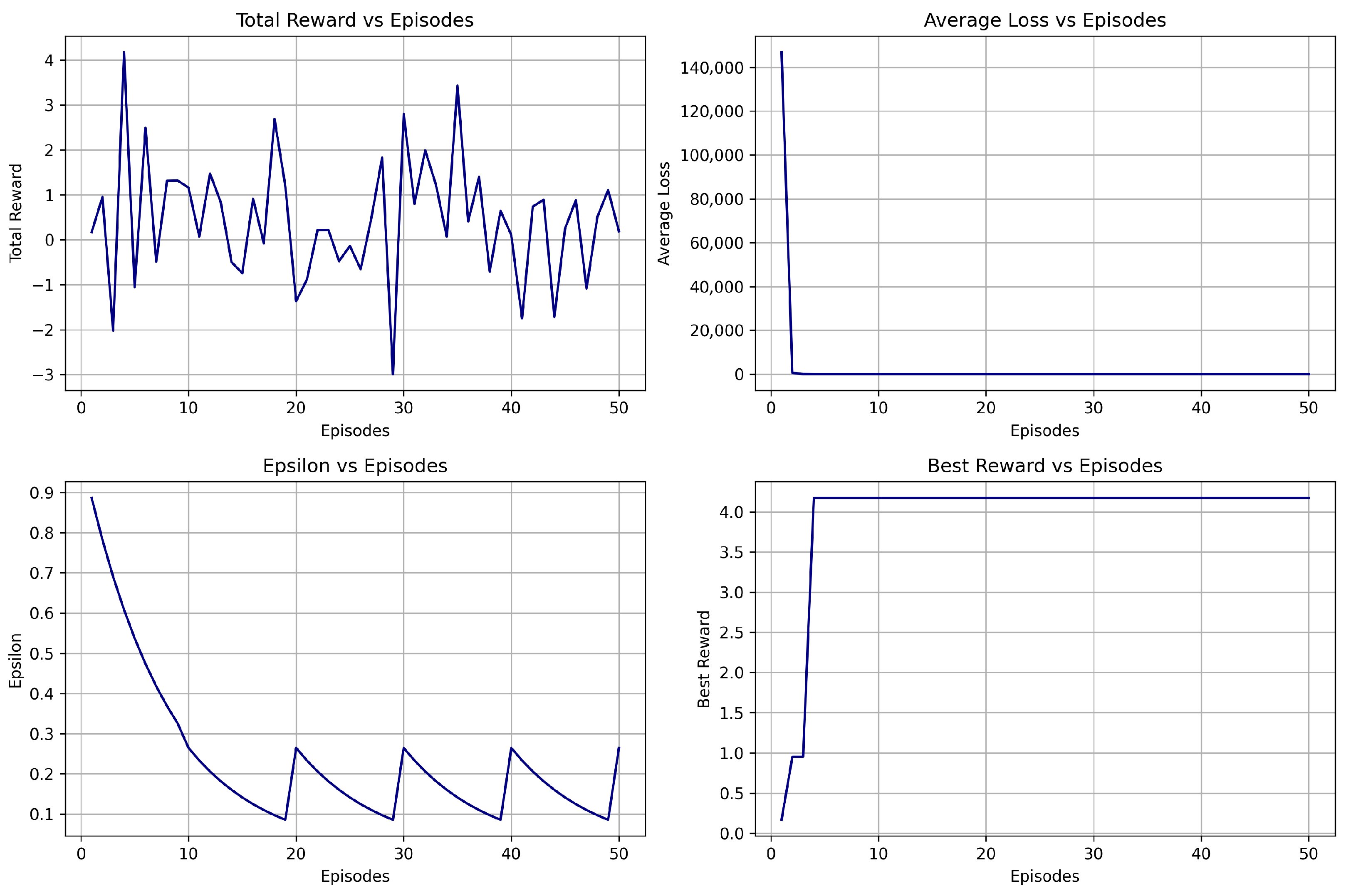
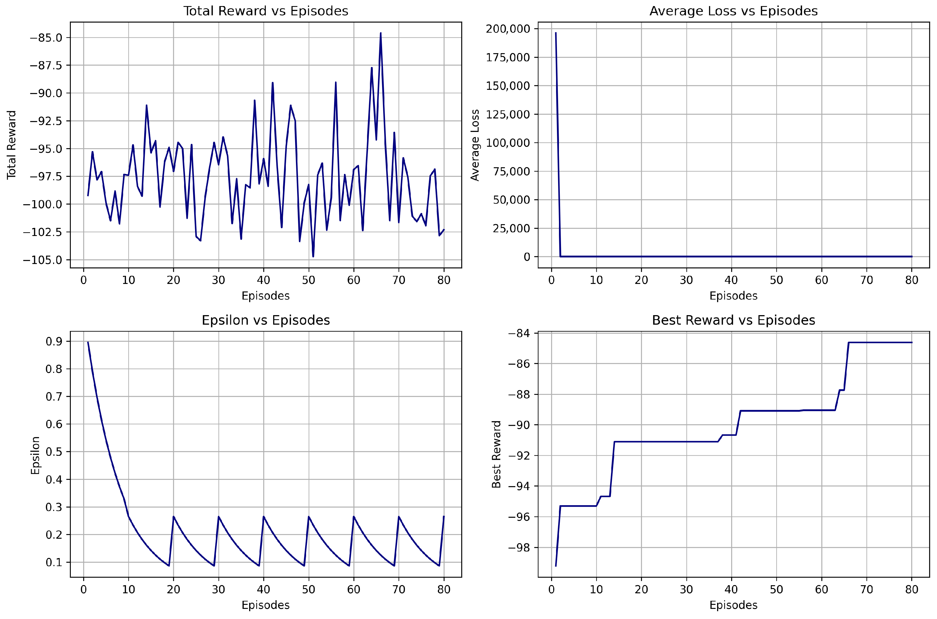
The training outcomes varied across DQN variants. DQN V1 showed the fastest convergence and delivered the best cumulative reward. DQN V2’s stability improved with epsilon resets, while DQN V3 demonstrated more balanced yet constrained learning due to softmax sampling and cooldown logic. Although V3 underperformed in raw rewards, its training curve exhibited reduced volatility and more cautious trade decisions. A comparison of the key features of the different DQN variants is provided in Table 4. The performance summary of the DQN models is shown in Table 5. The training performance plots for DQN versions V1, V2, and V3 are presented in Figure 2, Figure 3 and Figure 4, respectively.

6.1.4. Evaluation Summary on Test Data

On the test data, DQN V2 executed the highest number of trades (251), followed by DQN V1 (38) and DQN V3 (12). Despite its relatively lower trading frequency, DQN V1 achieved the highest win rate of 65.8% and yielded the best final balance of INR 329,737.81 (∼USD 3818). Despite fewer trades, DQN V3 delivered the highest Sharpe ratio (0.1126) and profit factor (1.37), reflecting efficient volatility-adjusted returns. In contrast, DQN V2 exhibited high trading activity but delivered only moderate profitability. To benchmark performance, all DQN models were compared against two rule-based baselines. The primary baseline, buy–hold–sell, executed a single trade resulting in a loss, with a final balance of INR 188,111.00 (∼USD 2178) and a Sharpe ratio of −0.459. The secondary baseline, based on a 50–200 EMA crossover strategy, executed 14 trades with a win rate of 50%, a profit factor of 1.12, a Sharpe ratio of 0.074, and a final balance of INR 227,730.00 (∼USD 2636). These findings demonstrate that all DQN variants outperformed the buy–hold–sell baseline, while DQN V1 also surpassed the 50–200 EMA crossover in terms of both profitability and Sharpe ratio. Table 6 compares trading metrics across baseline strategies and DQN variants. Among the DQN models, V3 achieved the highest profit factor (1.37) and Sharpe ratio (0.1126), reflecting better risk-adjusted returns, albeit on a lower trade count. DQN V1 displayed a balanced win rate (65.8%) with a moderate profit factor (1.35), while DQN V2, despite the highest trade frequency, had a comparatively weaker Sharpe ratio. These results suggest that aggressive trade execution without reward refinement may degrade model robustness in real-world settings. Figure 5 presents a comparative analysis of the equity curves for the three DQN versions, highlighting their trading performance over time. DQN V3’s curve is the steepest initially, showing rapid early gains but flattening with minimal drawdown, indicating conservative but stable policy behavior. DQN V1 shows a consistent upward trend, though less steep. DQN V2, despite more trades, demonstrates higher volatility with frequent reversals, resulting in the lowest ending balance among the three.

6.1.5. Transition to Advanced Architectures

Given the limitations observed in DQN, particularly its tendency for Q-value overestimation and fragile response to reward design, the study proceeds with the implementation and evaluation of DDQN and Dueling DDQN architectures, which are expected to address these issues. The following section evaluates DDQN, which addresses these shortcomings by decoupling action selection and value estimation.

6.2. Double Deep Q-Network (DDQN)

This section presents the experimental findings from the DDQN models, which build upon the foundational DQN architecture by addressing overestimation bias and stabilizing policy learning in the context of algorithmic trading on the NIFTY 50 dataset. Three variations of DDQN were implemented, each incorporating progressive enhancements in exploration strategy, action selection, and trade management to evaluate their impact on model performance and stability.

6.2.1. Hyperparameters

The DDQN variants shared a similar initialization pipeline to the DQN models but featured enhanced exploration strategies. V1 and V2 used a 10-step window, while V3 expanded to 100. V3 also reduced its learning rate to 0.00025 to stabilize training. All variants utilized prioritized experience replay and time/frequency-based reward penalties. V3 uniquely integrated softmax sampling, cooldown logic, and a reduced penalty coefficient to strike a balance between exploration and policy conservatism. The hyperparameters for the three DDQN versions are summarized in Table 7. Compared to the DQN counterparts, all DDQN versions retain prioritized replay and reward shaping, but they differ in use of softmax sampling and input window size. DDQN V3 mirrors the DQN V3’s deeper input horizon and modified optimizer behavior, aligning the architectural experimentation across both model families. This design enables a controlled comparison of base DQN and its enhanced versions, isolating the influence of reward tuning and exploration methods on trading efficiency.

6.2.2. Model Variants

  • DDQN V1 is the baseline model with prioritized experience replay and steady epsilon decay.
  • DDQN V2 incorporates periodic epsilon resets to encourage exploration in later episodes.
  • DDQN V3 integrates softmax action sampling, cooldown logic, and a reduced over-trading penalty to enhance stability and profitability.

6.2.3. Training Summary

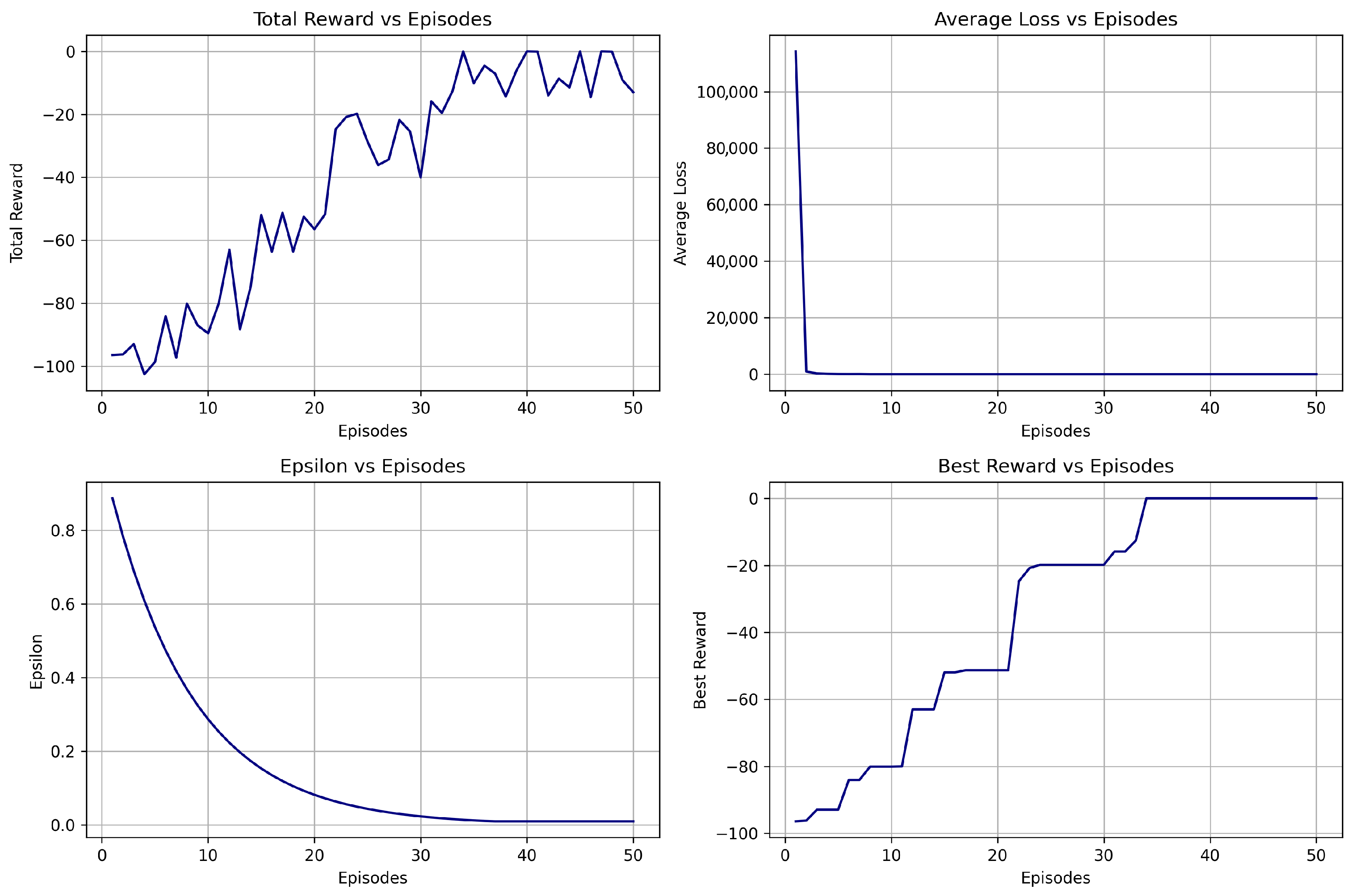
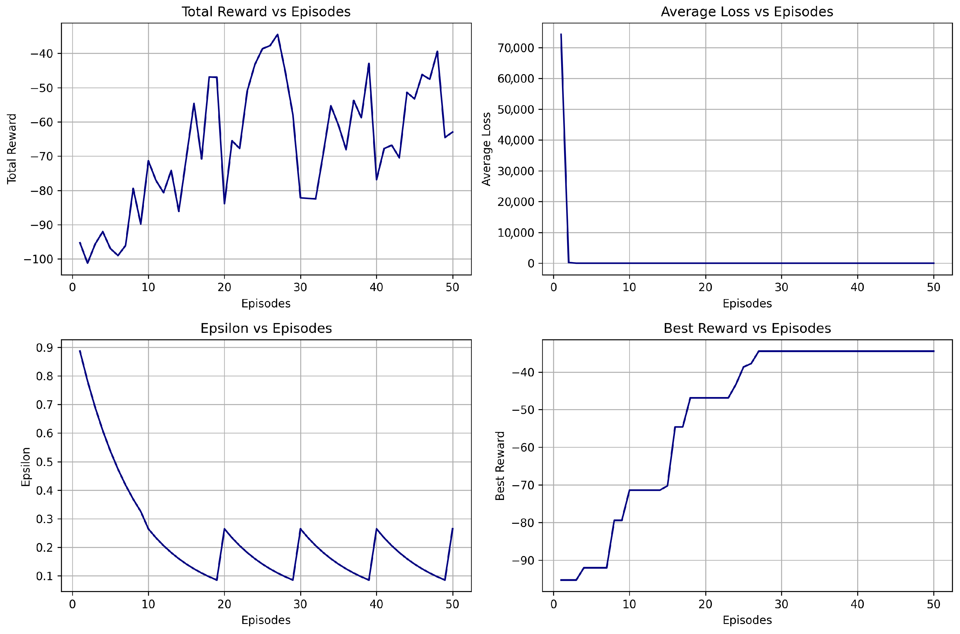
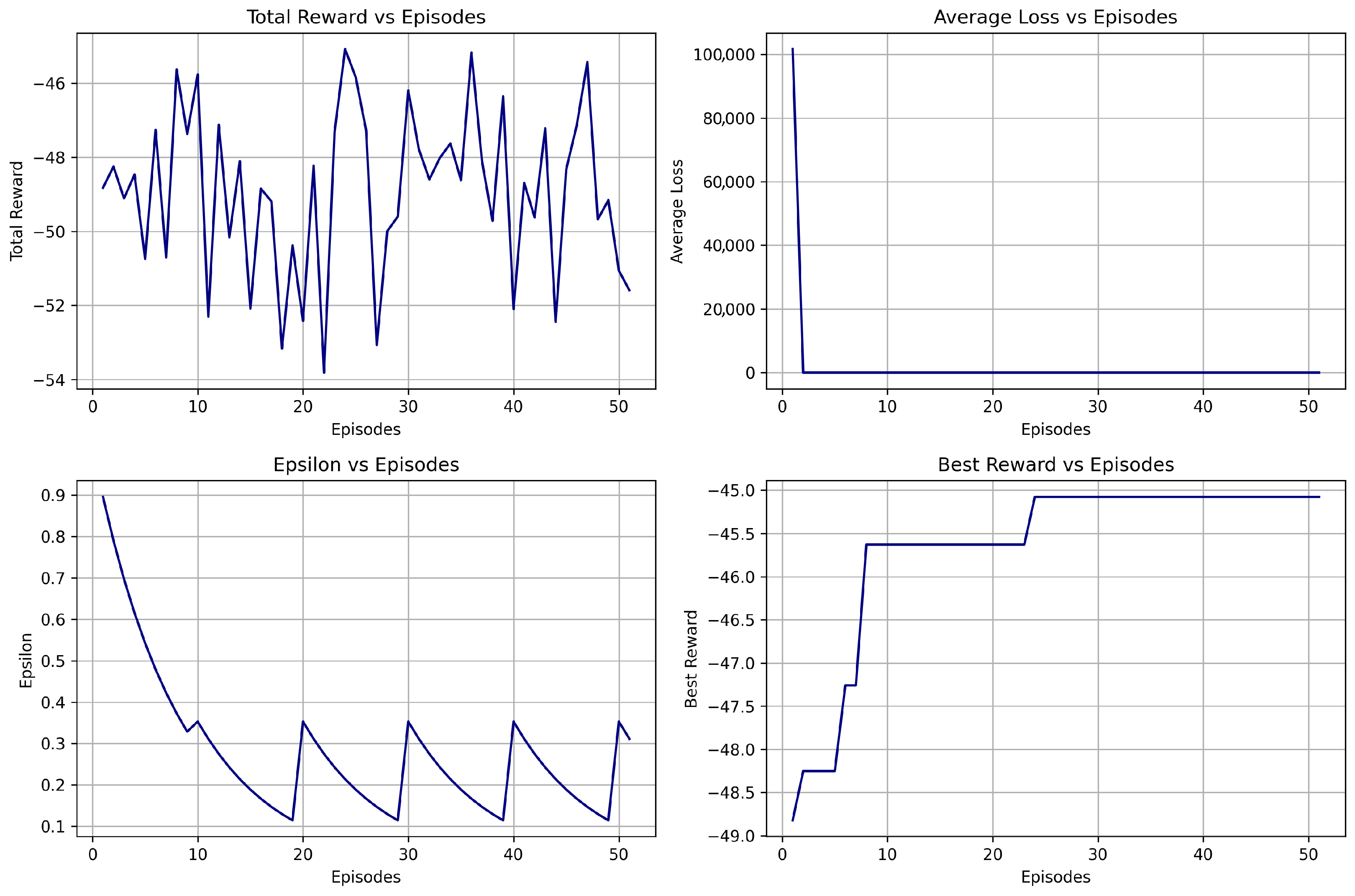
DDQN V1 displayed steady but moderate performance, while V2 benefited from periodic epsilon resets that promoted better exploration. V3 significantly outperformed its predecessors, achieving stable and consistent learning with an improved Sharpe ratio. The training logs indicated that the inclusion of softmax sampling and cooldown mechanisms in V3 helped avoid overfitting and led to more profitable policy trajectories. A comparison of the key features of the different DDQN variants is provided in Table 8. The performance summary of the DDQN models is shown in Table 9. The training performance plots for DDQN versions V1, V2, and V3 are presented in Figure 6, Figure 7 and Figure 8, respectively.

6.2.4. Evaluation Summary on Test Data

DDQN V3 recorded the best Sharpe ratio (0.7394), the highest final balance of INR 270,156 (∼USD 3128), and a strong win rate (73.3%) while limiting its activity to 15 high-quality trades. In contrast, V1 and V2 executed more trades but yielded lower returns and Sharpe ratios. V3’s improved volatility-adjusted performance positions it as the most balanced and practical model. DDQN V3 outperformed both baselines in terms of overall profitability, win rate, and Sharpe ratio. It stands out as the most balanced and deployment-ready model in this class. The summary of the trading performance for all three DDQN models is shown in Table 10. Figure 9 presents a comparative analysis of the equity curves for the three DDQN versions, highlighting their trading performance over time.

6.2.5. Transition to Advanced Architectures

Given the observed performance of DDQN variants, particularly the improvements achieved with softmax sampling and cooldown logic in V3, the study proceeds with the implementation and evaluation of Dueling DDQN to further enhance learning efficiency and policy stability in the dynamic NIFTY 50 trading environment.

6.3. Dueling Double Deep Q-Network (Dueling DDQN)

This section presents the experimental findings from the Dueling DDQN models, which extend the DDQN architecture by introducing separate value and advantage streams to refine Q-value estimates and enhance policy learning. Three variations of Dueling DDQN were implemented, each incorporating progressive enhancements in exploration strategy, action selection, and trade management to evaluate their impact on model performance and stability in the context of algorithmic trading on the NIFTY 50 index.

6.3.1. Hyperparameters

The Dueling DDQN models maintained the foundational settings of the DDQN pipeline with architectural extensions. Specifically, the network bifurcated into separate value and advantage streams after the shared layers. All variants adopted prioritized experience replay, epsilon decay, and reward shaping. V3 used a larger input window (100 timesteps), softmax sampling, and cooldown logic. The hyperparameters for the three Dueling DDQN versions are summarized in Table 11.

6.3.2. Model Variants

  • Dueling DDQN V1 is the baseline model with prioritized experience replay and steady epsilon decay.
  • Dueling DDQN V2 incorporates periodic epsilon resets to encourage exploration and prevent local optima entrapment.
  • Dueling DDQN V3 integrated softmax action sampling, cooldown logic, and a reduced reward penalty structure to balance exploration–exploitation trade-offs and enhance policy stability.

6.3.3. Training Summary

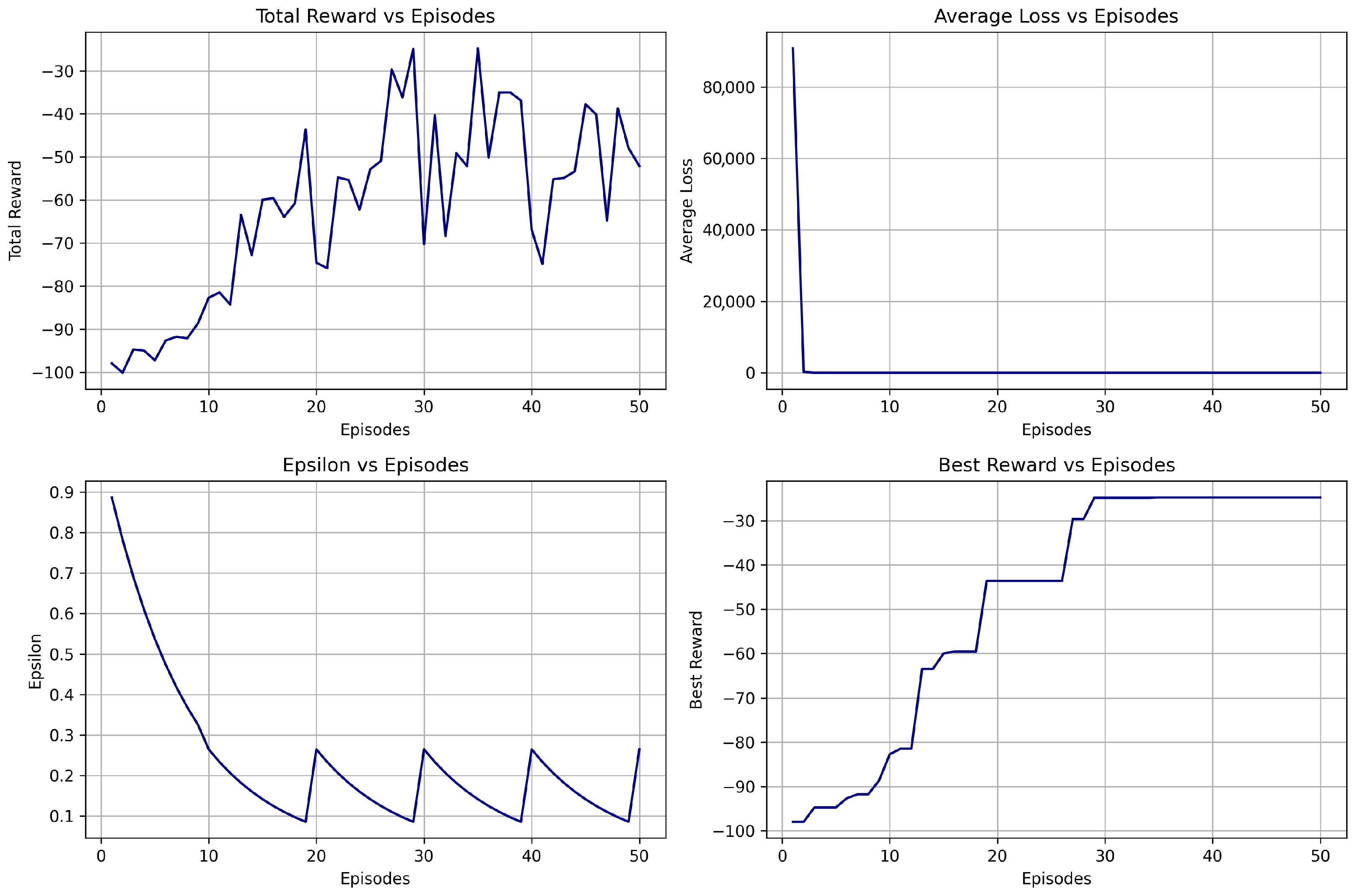
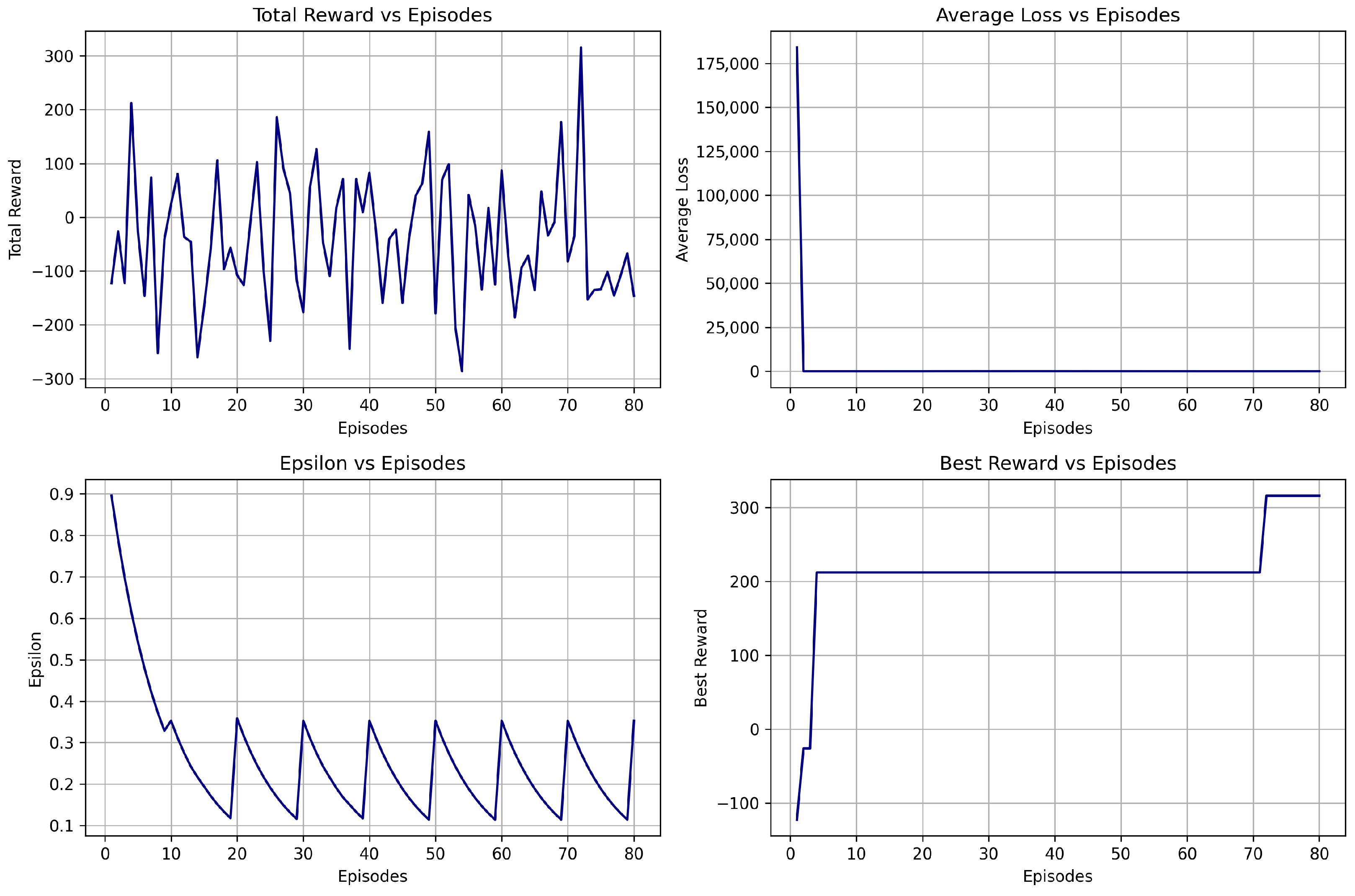
Among the dueling variants, V3 achieved the highest learning efficiency, converging quickly and consistently to profitable policies. While V1 exhibited moderate reward trajectories and V2 showed slightly more stable exploration, only V3 demonstrated significant gains in Sharpe ratio and minimized reward volatility. These improvements were driven by the combination of softmax-based exploration and cooldown mechanisms, which regulated trade frequency. The performance summary of the Dueling DDQN models is shown in Table 12. The training performance plots for Dueling DDQN versions V1, V2, and V3 are presented in Figure 10, Figure 11 and Figure 12, respectively.

6.3.4. Evaluation Summary on Test Data

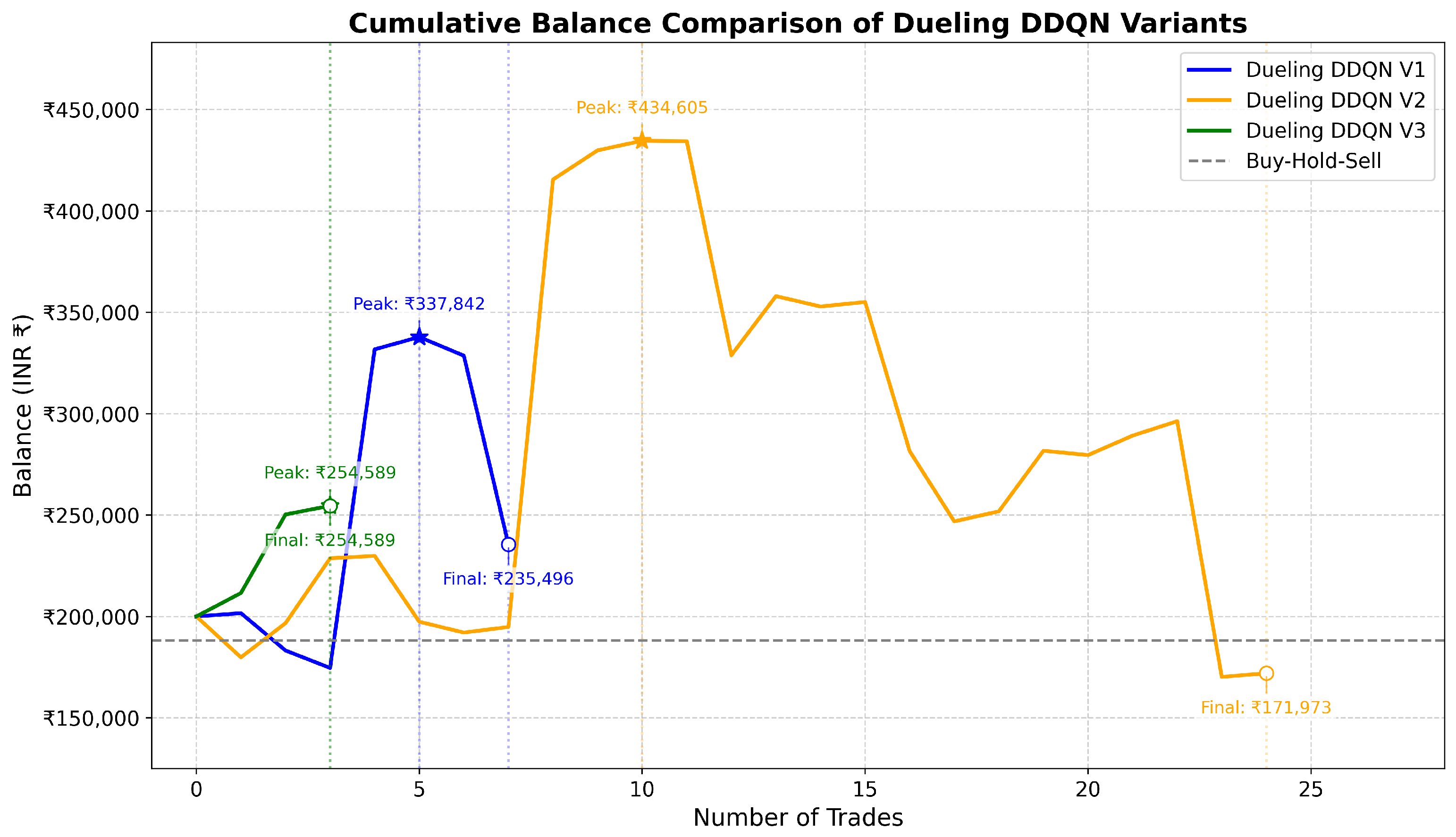
Dueling DDQN V3 achieved an exceptional Sharpe ratio (1.2278) and a perfect win rate (100%) across just three trades, indicating highly selective yet profitable decision-making. Dueling DDQN V3 also outperformed both baselines in terms of final balance and Sharpe ratio. In contrast, V1 and V2 showed lower win rates and executed more trades of varying quality. The undefined profit factor observed in V3 resulting from a low number of trades with no losses should be interpreted with caution due to the limited sample size. Nonetheless, these results underscore the potential of selective DRL strategies like V3 for precision trading in volatile market environments. The summary of the trading performance for all three Dueling DDQN models is shown in Table 13. Figure 13 presents a comparative analysis of the equity curves for the three Dueling DDQN versions, highlighting their trading performance over time.

6.4. Cross-Model Performance Metrics

This section provides a comparative analysis of the three selected reinforcement learning models, i.e., DQN (V1), DDQN (V3), and Dueling DDQN (V3), based on both training performance and final evaluation metrics. The goal is to identify the most effective architecture for generating robust trading signals on the NIFTY 50 index.

6.4.1. Evaluation Metrics Comparison

Table 14 summarizes key performance metrics across the three model variants, including total trades, win rate, profit factor, Sharpe ratio, final balance, mean profit/loss (PnL) per trade, and its 95% confidence interval (CI).
While DQN (V1) executed the highest number of trades (38), it delivered a relatively low Sharpe ratio (0.097) and a modest mean PnL of INR 3414.15 (∼USD 39.50). The wide 95% CI (INR −8416.31, INR 14,265.13) suggests considerable variability and the potential for negative returns. DDQN (V3) demonstrated improved performance, with 15 trades and a higher win rate of 73.33%. It achieved a mean PnL of INR 4677.06 (∼USD 54.10) and a narrower CI (INR 1739.27, INR 8071.12), offering greater statistical confidence in its profitability. Its Sharpe ratio of 0.739 confirms an improved risk–return trade-off. Dueling DDQN (V3) achieved the highest mean PnL of INR 18,196.25 (∼USD 210.60) and Sharpe ratio of 1.228. However, this was based on just three trades, all profitable. Consequently, the profit factor is undefined (NA) due to the absence of any losses, and the 95% CI (INR 4294.68, INR 38,730.00) is extremely wide, underscoring the statistical uncertainty. This highlights the need for caution when interpreting metrics based on sparse trades.

6.4.2. Training Stability Analysis

The training logs reveal notable differences in learning stability. DQN (V1) showed moderate total rewards, with gradual convergence and consistent exploration. Training losses decreased smoothly, suggesting stable learning but also indicating potential overestimation bias. DDQN (V3) exhibited more volatile training rewards early on but gradually stabilized as exploration strategies like softmax sampling and cooldown logic were introduced. The integration of periodic epsilon resets and optimized learning rates improved exploration–exploitation balance and led to a significant gain in Sharpe ratio (0.739). Dueling DDQN (V3) displayed significant variance in total rewards across episodes, with occasional large profit spikes (e.g., 212.09 reward at episode 4). While the Sharpe ratio reached 1.228, the result is based on only three trades, which may reflect insufficient exploration of trading opportunities.

6.4.3. Overall Model Performance

From a practical trading perspective, the models can be compared along several dimensions. DQN (V1) had the highest trade count, indicating higher market activity but with lower volatility-adjusted returns compared to DDQN (V3). DDQN (V3) provided the highest volatility-adjusted returns while maintaining a moderate trade count, indicating a trade-off between profitability and trade quality. Dueling DDQN (V3) showed promising volatility-adjusted metrics but with too few trades for meaningful statistical confidence. This suggests that additional experiments with alternative exploration strategies or modifications to the reward function may yield improved results.

7. Discussion

7.1. DQN Model: Interpretation and Key Insights

The results of DQN training and evaluation reveal several insights. Among the three variants, DQN V1 demonstrated the most stable convergence and highest profitability, making it a suitable benchmark for comparison. DQN V2, despite its high trade frequency, suffered from a lower Sharpe ratio and win rate, suggesting that aggressive trading without proper regularization may reduce real-world performance. DQN V3, though more conservative in behavior, achieved the highest Sharpe ratio and profit factor, which indicates better risk-adjusted returns despite fewer trades.
The reward shaping and softmax-based exploration strategies used in DQN V3 required careful tuning. The combined effect of cooldown logic and penalties made the model stable, but also limited its responsiveness to changing market conditions. In contrast, the absence of such controls in DQN V2 led to noisier and less consistent trading patterns.
Overall, the results highlight a trade-off between model complexity and responsiveness. DQN V1, although simpler, performed reliably and remains a strong baseline for comparison due to its consistent results and balanced trading behavior.

7.2. DDQN Model: Interpretation and Key Insights

The DDQN models demonstrated meaningful improvements over their DQN counterparts, particularly in terms of exploration efficiency and volatility-adjusted returns. The inclusion of periodic epsilon resets in V2 and advanced exploration strategies like softmax sampling and cooldown logic in V3 helped in mitigating overestimation bias and improving policy stability. Among the three versions, DDQN V3 emerged as the most robust variant, achieving a high Sharpe ratio (0.7394), a win rate of 73.3%, and maintaining restrained trading activity with only 15 trades. This indicates a balance between profitability and risk, with higher-quality trade execution and minimal drawdown.
The lower trade count of V3, when compared to V1 and V2, suggests improved selectivity and better control over trading risks, which is essential for real-world deployment. In contrast to DQN V1, which had higher raw profit but a weaker Sharpe ratio, DDQN V3 shows a more balanced trade-off between return and risk. These results support observations in recent literature, where improvements in exploration and policy regularization have led to more stable DRL performance under noisy and dynamic market conditions.
However, the improvement in V3’s risk-adjusted metrics comes with slightly more conservative behavior. The combined effect of softmax sampling and cooldown logic, while effective in controlling overtrading, may reduce the model’s responsiveness in rapidly changing market scenarios.

7.3. Dueling DDQN Model: Interpretation and Key Insights

The experimental results for the Dueling DDQN architecture reveal that the inclusion of value and advantage streams significantly enhances the agent’s decision-making capability. Among the three variants, Dueling DDQN V3 stood out by achieving the highest Sharpe ratio (1.2278) and a perfect win rate (100%) over three trades, despite its minimal trading activity. While the small number of trades limits the statistical significance of its performance metrics, the results point towards a highly selective and risk averse policy, which are characteristics that are desirable in volatile or low liquidity environments.
The improvement in V3 is primarily attributed to the combined effect of softmax sampling and cooldown logic. These components contributed to a more cautious yet profitable trading pattern, reducing the tendency of overfitting observed in earlier variants. Softmax sampling encouraged diverse action exploration, while cooldown logic acted as a natural trade filter, helping the model focus on higher-quality trades. This is consistent with findings in earlier studies that support the use of exploration control in reinforcement learning-based trading systems.
However, the sharp contrast between V3’s performance and the relatively weaker results of V1 and V2 also indicates sensitivity to hyperparameter tuning and reward shaping. While V1 and V2 executed more trades, they failed to produce strong risk-adjusted returns, suggesting that frequency alone is not a reliable indicator of model effectiveness. V2’s negative Sharpe ratio (−0.0194), despite its 58.33% win rate, highlights the importance of balancing win frequency with risk reward tradeoffs.
In summary, the dueling architecture, especially when combined with improved exploration strategies, demonstrates strong potential for strategic trade selection. Nevertheless, the limited number of trades in the best-performing variant (V3) suggests the need for further testing across longer horizons and different market conditions to better assess its robustness and practical utility.

7.4. Comparison with Existing Literature

To contextualize our contribution, Table 15 summarizes key attributes of recent DRL-based trading studies, including dataset scope, temporal resolution, performance metrics like Sharpe ratio, and comparative baselines.
Many existing research papers explore similar DRL-based trading strategies but apply them to different datasets, typically from foreign markets or alternative asset classes such as the S&P 500, DJIA, etc. In contrast, the proposed study focuses specifically on the Indian NIFTY 50 index, which remains largely underrepresented in DRL literature. To the best of our knowledge, this is the first comprehensive application of DRL models to include DQN, DDQN, and Dueling DDQN on the Indian NIFTY 50 index using high-frequency 15-min OHLC data and evaluated against statistical baselines using Sharpe Ratio, equity curves, and confidence intervals. While most prior works rely on daily price data, our approach allows more granular and responsive intraday decision-making. Additionally, unlike studies that evaluate a single DRL model in isolation, we systematically benchmark three DRL architectures under a unified framework. Risk-adjusted performance metrics such as Sharpe ratio that are often omitted or loosely reported are explicitly calculated and reported (0.097 for DQN, 0.739 for DDQN, and 1.228 for Dueling DDQN), with supporting statistics including confidence intervals and profit factor. Finally, we incorporate real-world constraints such as brokerage costs and margin requirements into our evaluation, enhancing the practical relevance and deployability of the results. Together, these methodological and empirical advancements distinguish our work from existing DRL-based financial studies.

7.5. Cross-Model Performance Interpretation

Building upon the comparative analysis, this subsection offers strategic recommendations based on the observed behavior and real-world suitability of each model. The results across the three selected models, namely DQN (V1), DDQN (V3), and Dueling DDQN (V3), clearly highlight the differences in their learning behaviors and trading outcomes. DQN (V1) executed the highest number of trades, indicating its aggressive exploration nature, but this also led to a moderate Sharpe ratio. On the other hand, DDQN (V3) managed to strike a better balance between trade count and profitability, reflected through a high Sharpe ratio and win rate. This improvement can be attributed to the use of exploration techniques like softmax sampling and cooldown logic, which helped the model reduce overestimation bias and make more stable decisions.
Dueling DDQN (V3) achieved the highest Sharpe ratio among all models along with a perfect win rate. However, its performance was based on only three trades, which raises questions about the statistical reliability of the outcome. It appears that the Dueling DDQN variant became too conservative due to its stricter exploration and reward constraints, resulting in missed opportunities. In comparison, DDQN (V3) maintained an appropriate trade frequency with better control over risks, making it the most balanced model in terms of performance and generalization. This comparative analysis shows that while all models have their strengths, the practical choice would depend on the trade-off between risk appetite, frequency of trades, and return consistency.

7.6. Strategic Recommendations and Practical Considerations

While the models show encouraging results in backtesting, it is essential to reflect on the practical considerations and limitations that may arise in live deployment. DQN (V1) continues to serve as a strong baseline model and demonstrates decent performance when compared to traditional rule-based strategies. However, it suffers from overestimation bias and a lower Sharpe ratio, which limits its effectiveness in high-volatility conditions. DDQN (V3) emerges as the most balanced and practically deployable model due to its improved Sharpe ratio, better win rate, and moderate number of trades. It shows consistent profitability while maintaining stability in training and evaluation. On the other hand, Dueling DDQN (V3), despite showing the highest Sharpe ratio and a perfect win rate, executed only a few trades, which raises questions about the reliability of its performance. This model would benefit from further hyperparameter tuning and increased trade volume to fully utilize its architectural improvements.
Based on our findings, DDQN (V3) is recommended as the most suitable benchmark for future developments and potential real-world deployment. Its results indicate a good trade-off between risk and return, and it is likely to perform reliably under different market conditions.
While the strategies performed well during backtesting, their application in live markets comes with additional challenges. Slippage and delay in order execution can impact profits, especially during periods of high volatility. In our setup, we have considered realistic elements such as brokerage charges, margin requirements, and the minimum capital needed to hold a single lot overnight. However, other practical factors like execution latency, partial fills, and order book dynamics were not simulated and may influence real-world performance. These aspects should be considered by practitioners before deploying any of the models in a live trading environment.

7.7. Study Limitations and Constraints

While this study offers a promising direction for developing intelligent trading systems in emerging markets, it is important to acknowledge several limitations associated with the current research setup. Although the proposed framework incorporates realistic constraints such as initial capital, margin requirements, and brokerage charges, it is based entirely on backtesting with historical data. As such, critical aspects of live trading, including slippage, bid–ask spread, order execution delays, and real-time latency, are not captured. Other dynamic factors such as partial fills, market depth, and liquidity fluctuations were also not simulated, which may significantly influence actual trading performance, especially in high-frequency settings.
Another limitation lies in the low number of trades executed by some model variants, particularly Dueling DDQN (V3). While it showed a perfect win rate and the highest Sharpe ratio, the statistical significance of these metrics is limited. The small trade count might indicate an overly cautious policy that could miss profitable opportunities in more active market conditions. Further experimentation over longer timeframes is needed to assess its reliability and generality.
The study also focuses exclusively on a single market index, the NIFTY 50. Although it is a strong representative of the Indian stock market, the conclusions drawn may not directly transfer to individual equities, mid-cap indices, commodities, or foreign markets. Broader testing across asset classes is necessary to validate models’ applicability. Additionally, the hyperparameters in this study were selected through manual trial and error. A more systematic tuning process could potentially yield better performance and reduce the risk of suboptimal learning.
Furthermore, the current models are trained as single-agent systems without accounting for interactions with other market participants. Real markets are multi-agent and dynamic in nature, where strategies adapt continuously. Also, the decision-making process in the models is not inherently explainable, which may limit their acceptance in institutional settings where transparency and risk control are essential.
Despite these limitations, the study provides a strong foundation for building DRL-based trading systems tailored to the Indian context.

8. Conclusion and Future Work

Conventional econometric models such as ARDL, ARIMA, ARCH, and GARCH have been widely used to detect anomalies and trends in stock market movements. These methods, while effective in analyzing historical data and volatility, are often limited in their ability to adapt to the rapidly evolving dynamics of modern financial markets, particularly in high-frequency trading scenarios. Despite the recent surge in DRL-based trading strategies globally, few studies have systematically explored their deployment in emerging markets like India, especially using real-world, high-frequency market data. Additionally, most prior works lack comprehensive risk-adjusted evaluation, making their findings difficult to translate into deployable systems. To address this gap, this study employed three DRL approaches, DQN, DDQN, and Dueling DDQN, to model and analyze market behavior.
Among the models evaluated, DDQN (V3) exhibited consistent performance in terms of volatility-adjusted returns, reflected by favorable Sharpe ratios and more stable learning behavior. The Dueling DDQN (V3) variant also produced encouraging outcomes; however, the limited number of executed trades raises questions regarding statistical robustness. DQN (V1) served as a useful baseline, highlighting known issues such as overestimation bias and less-effective risk management.
Our study contributes to the literature by providing a systematic comparison of DRL variants using a decade-long, high-frequency dataset from the Indian NIFTY 50 index. The integration of softmax sampling, cooldown logic, and reward–penalty mechanisms demonstrates how architectural and policy-level enhancements can directly improve model robustness, trade quality, and risk-adjusted performance.
While the findings suggest that DDQN-based approaches have the potential to assist investors in managing market volatility and generating alpha, it is important to note that these results are based on backtested simulations. Therefore, any claims regarding their real-world deployment readiness should be made with caution. The absence of live-market implementation limits the conclusions that can be drawn about their practical applicability at this stage.
Future work will aim to strengthen the framework in several directions. First, the reward function will be enhanced by incorporating dynamic, market-aware risk metrics to improve real-time decision-making. Second, the models will be evaluated across other stock indices and asset classes to assess their generalizability. Third, hybrid architectures, incorporating attention mechanisms or transformer-based layers, will be explored to better capture temporal dependencies in financial data. Importantly, future research will also focus on testing these models in live or simulated trading environments with real-time feedback loops. Additionally, applying the proposed methods to other emerging markets will help examine their adaptability and effectiveness under different economic and regulatory conditions.
Finally, this framework opens new directions for practitioners and researchers seeking robust, data-driven trading systems tailored for high-frequency, volatile markets. The model configurations, evaluation benchmarks, and empirical insights established here serve as a replicable foundation for future algorithmic trading research in both academic and applied finance settings.

Author Contributions

Conceptualization, R.G.M., D.S. and M.G.; methodology and software, R.G.M.; validation, D.S. and M.G.; writing—original draft preparation, R.G.M., D.S. and M.G.; supervision and writing—review and editing, S.P. and A.K. All authors have read and agreed to the published version of the manuscript.

Funding

This research received no external funding.

Institutional Review Board Statement

Not applicable.

Informed Consent Statement

Not applicable.

Data Availability Statement

The data that support the findings of this study are available on GitHub at https://github.com/rajgmishra/nifty50-15min-ohlc (accessed on 5 July 2025).

Conflicts of Interest

The authors declare no conflicts of interest.

References

  1. Economic Times. Every 4th Rupee in Mutual Funds Belong to Retail Investors, HNIs Own 1/3rd AUM: Franklin Templeton India MF. Economic Times. 6 February 2024. Available online: https://economictimes.indiatimes.com/mf/mf-news/every-4th-rupee-in-mutual-funds-belong-to-retail-investors-hnis-own-1/3rd-aum-franklin-templeton-india-mf/articleshow/122833651.cms (accessed on 23 July 2025).
  2. Ansari, Y.; Yasmin, S.; Naz, S.; Zaffar, H.; Ali, Z. A Deep Reinforcement Learning-Based Decision Support System for Automated Stock Market Trading. IEEE Access 2022, 10, 133228–133238. [Google Scholar] [CrossRef]
  3. Ryll, L.; Seidens, S. Evaluating the Performance of Machine Learning Algorithms in Financial Market Forecasting: A Comprehensive Survey. arXiv 2019. [Google Scholar] [CrossRef]
  4. Pricope, T.-V. Deep Reinforcement Learning in Quantitative Algorithmic Trading: A Review. arXiv 2021. [Google Scholar] [CrossRef]
  5. Awad, A.L.; Elkaffas, S.M.; Fakhr, M.W. Stock Market Prediction Using Deep Reinforcement Learning. Appl. Syst. Innov. 2023, 6, 106. [Google Scholar] [CrossRef]
  6. Nuipian, W.; Meesad, P.; Maliyaem, M. Innovative Portfolio Optimization Using Deep Q-Network Reinforcement Learning. In Proceedings of the 2024 8th International Conference on Natural Language Processing and Information Retrieval (NLPIR ’24), Okayama, Japan, 13–15 December 2024; pp. 292–297. [Google Scholar] [CrossRef]
  7. Du, S.; Shen, H. A Stock Prediction Method Based on Deep Reinforcement Learning and Sentiment Analysis. Appl. Sci. 2024, 14, 8747. [Google Scholar] [CrossRef]
  8. Hossain, F.; Saha, P.; Khan, M.; Hanjala, M. Deep Reinforcement Learning for Enhanced Stock Market Prediction with Fine-Tuned Technical Indicators. In Proceedings of the 2024 IEEE International Conference on Computing, Applications and Systems (COMPAS), Cox’s Bazar, Bangladesh, 25–26 September 2024; pp. 1–8. [Google Scholar] [CrossRef]
  9. Sagiraju, K.; Mogalla, S. Deployment of Deep Reinforcement Learning and Market Sentiment Aware Strategies in Automated Stock Market Prediction. Int. J. Eng. Trends Technol. 2022, 70, 37–47. [Google Scholar] [CrossRef]
  10. Mienye, E.; Jere, N.; Obaido, G.; Mienye, I.D.; Aruleba, K. Deep Learning in Finance: A Survey of Applications and Techniques. AI 2024, 5, 2066–2091. [Google Scholar] [CrossRef]
  11. Hu, Z.; Zhao, Y.; Khushi, M. A Survey of Forex and Stock Price Prediction Using Deep Learning. Appl. Syst. Innov. 2021, 4, 9. [Google Scholar] [CrossRef]
  12. Hiransha, M.; Gopalakrishnan, E.A.; Menon, V.K.; Soman, K.P. NSE Stock Market Prediction Using Deep-Learning Models. Procedia Comput. Sci. 2018, 132, 1351–1362. [Google Scholar] [CrossRef]
  13. Yang, H.; Liu, X.Y.; Zhong, S.; Walid, A. Deep Reinforcement Learning for Automated Stock Trading: An Ensemble Strategy. In Proceedings of the 1st ACM International Conference on AI in Finance (ICAIF), New York, NY, USA, 15–16 October 2020; pp. 1–8. [Google Scholar]
  14. Zhang, Z.; Zohren, S.; Roberts, S. Deep Reinforcement Learning for Trading. J. Financ. Data Sci. 2020, 2, 25–40. [Google Scholar] [CrossRef]
  15. Singh, V.; Chen, S.S.; Singhania, M.; Nanavati, B.; Gupta, A. How Are Reinforcement Learning and Deep Learning Algorithms Used for Big Data-Based Decision Making in Financial Industries—A Review and Research Agenda. Int. J. Inf. Manag. Data Insights 2022, 2, 100094. [Google Scholar] [CrossRef]
  16. Kabbani, T.; Duman, E. Deep Reinforcement Learning Approach for Trading Automation in the Stock Market. IEEE Access 2022, 10, 93564–93574. [Google Scholar] [CrossRef]
  17. Théate, T.; Ernst, D. An Application of Deep Reinforcement Learning to Algorithmic Trading. Expert Syst. Appl. 2021, 173, 114632. [Google Scholar] [CrossRef]
  18. Li, Y.; Zheng, W.; Zheng, Z. Deep Robust Reinforcement Learning for Practical Algorithmic Trading. IEEE Access 2019, 7, 108014–108022. [Google Scholar] [CrossRef]
  19. Cheng, L.-C.; Huang, Y.-H.; Hsieh, M.-H.; Wu, M.-E. A Novel Trading Strategy Framework Based on Reinforcement Deep Learning for Financial Market Predictions. Mathematics 2021, 9, 3094. [Google Scholar] [CrossRef]
  20. Taghian, M.; Asadi, A.; Safabakhsh, R. Learning Financial Asset-Specific Trading Rules via Deep Reinforcement Learning. Expert Syst. Appl. 2022, 195, 116523. [Google Scholar] [CrossRef]
  21. Li, Y.; Ni, P.; Chang, V. Application of Deep Reinforcement Learning in Stock Trading Strategies and Stock Forecasting. Computing 2020, 102, 1305–1322. [Google Scholar] [CrossRef]
  22. Bajpai, S. Application of Deep Reinforcement Learning for Indian Stock Trading Automation. arXiv 2021. [Google Scholar] [CrossRef]
  23. Guéant, O.; Manziuk, I. Deep Reinforcement Learning for Market Making in Corporate Bonds: Beating the Curse of Dimensionality. Appl. Math. Financ. 2019, 26, 387–452. [Google Scholar] [CrossRef]
  24. Wang, H.; Zhou, X.Y. Continuous-Time Mean–Variance Portfolio Selection: A Reinforcement Learning Framework. Math. Financ. 2020, 30, 1015–1050. [Google Scholar] [CrossRef]
  25. Hambly, B.; Xu, R.; Yang, H. Recent Advances in Reinforcement Learning in Finance. Math. Financ. 2023, 33, 437–503. [Google Scholar] [CrossRef]
  26. Fu, Y.-T.; Huang, W.-C. Optimizing Stock Investment Strategies with Double Deep Q-Networks: Exploring the Impact of Oil and Gold Price Signals. Appl. Soft Comput. 2025, 180, 113264. [Google Scholar] [CrossRef]
  27. Carta, S.; Ferreira, A.; Podda, A.S.; Recupero, D.R.; Sanna, A. Multi-DQN: An Ensemble of Deep Q-Learning Agents for Stock Market Forecasting. Expert Syst. Appl. 2021, 164, 113820. [Google Scholar] [CrossRef]
  28. Huang, Y.; Lu, X.; Zhou, C.; Song, Y. DADE-DQN: Dual Action and Dual Environment Deep Q-Network for Enhancing Stock Trading Strategy. Mathematics 2023, 11, 3626. [Google Scholar] [CrossRef]
  29. Liu, W.; Gu, Y.; Ge, Y. Multi-Factor Stock Trading Strategy Based on DQN with Multi-BiGRU and Multi-Head ProbSparse Self-Attention. Appl. Intell. 2024, 54, 5417–5440. [Google Scholar] [CrossRef]
  30. Chen, X.; Wang, Q.; Hu, C.; Wang, C. A Stock Market Decision-Making Framework Based on CMR-DQN. Appl. Sci. 2024, 14, 6881. [Google Scholar] [CrossRef]
  31. Huang, Z.; Gong, W.; Duan, J. TBDQN: A Novel Two-Branch Deep Q-Network for Crude Oil and Natural Gas Futures Trading. Appl. Energy 2023, 347, 121321. [Google Scholar] [CrossRef]
  32. Chakole, J.B.; Kolhe, M.S.; Mahapurush, G.D.; Yadav, A.; Kurhekar, M.P. A Q-Learning Agent for Automated Trading in Equity Stock Markets. Expert Syst. Appl. 2021, 163, 113761. [Google Scholar] [CrossRef]
  33. Shi, Y.; Li, W.; Zhu, L.; Guo, K.; Cambria, E. Stock Trading Rule Discovery with Double Deep Q-Network. Appl. Soft Comput. 2021, 107, 107320. [Google Scholar] [CrossRef]
  34. Nagy, P.; Calliess, J.-P.; Zohren, S. Asynchronous Deep Double Dueling Q-Learning for Trading-Signal Execution in Limit Order Book Markets. Front. Artif. Intell. 2023, 6, 1151003. [Google Scholar] [CrossRef]
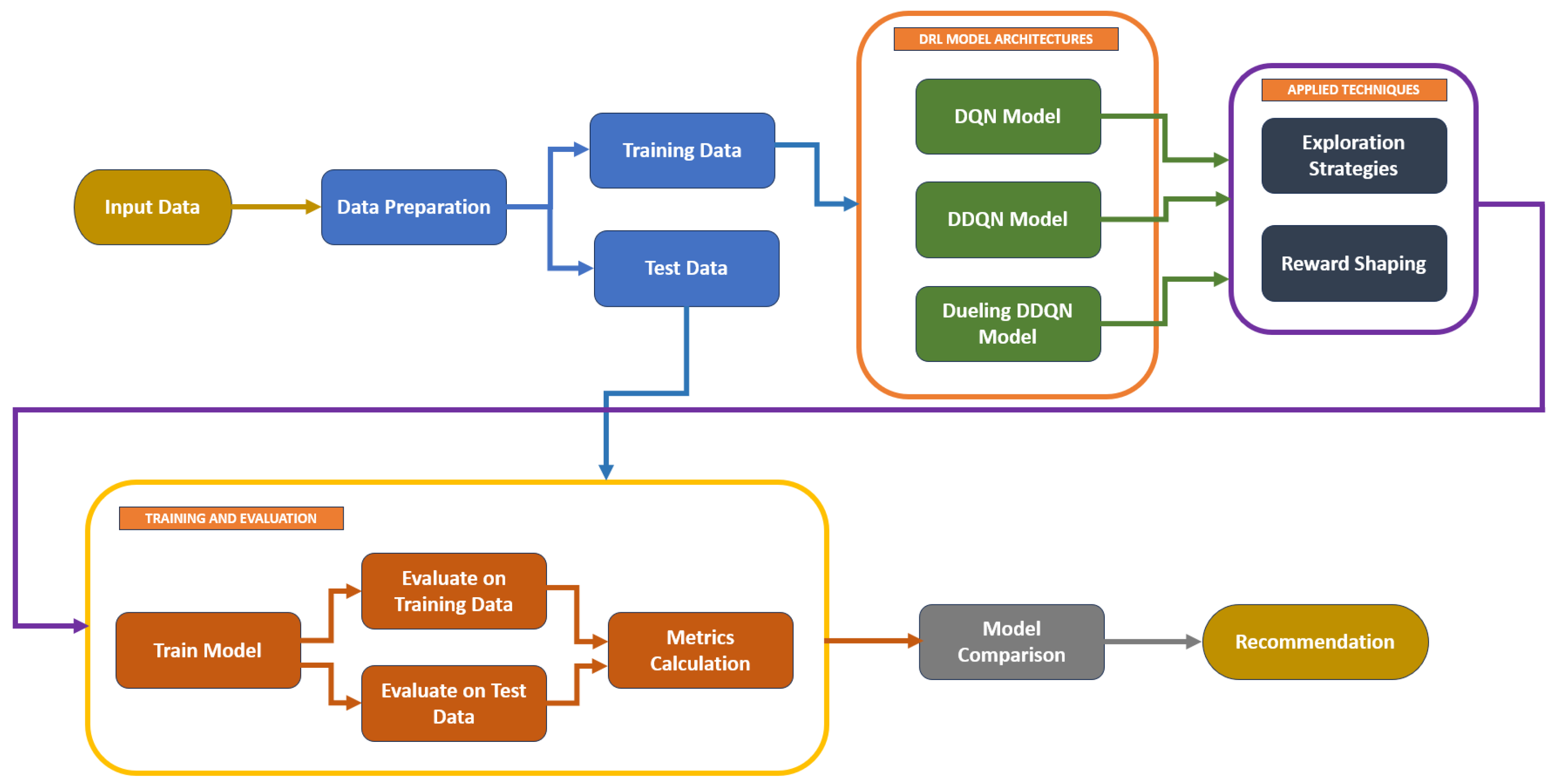
Figure 1. Research framework for a DRL-based trading strategy evaluation on the NIFTY 50 index. This diagram illustrates the sequential process from input data handling, model selection, application of exploration, and reward shaping techniques to model evaluation and recommendation.
Ai 06 00183 g001
Figure 2. Training performance of the DQN V1 baseline model with prioritized experience replay (PER). The plots in the figure show the reward trajectory and convergence behavior of the DQN V1 baseline model during training.
Ai 06 00183 g002
Figure 3. Training performance of the DQN V2 model with epsilon resets and a time-decay reward penalty. The plots in this figure illustrate how periodic exploration resets and regularization impact model’s learning stability.
Ai 06 00183 g003
Figure 4. Training performance of the DQN V3 model with softmax action sampling and cooldown logic. The plots in this figure demonstrate the stabilized but conservative model’s learning behavior due to advanced exploration strategies.
Ai 06 00183 g004
Figure 5. Equity curve comparison of DQN variants. This plot visualizes the portfolio growth achieved by DQN V1, V2, and V3 on test data.
Ai 06 00183 g005
Figure 6. Training performance of the DDQN V1 model with prioritized experience replay and steady epsilon decay. The plots in this figure highlight steady learning with moderate improvement in episodic rewards.
Ai 06 00183 g006
Figure 7. Training performance of the DDQN V2 model with periodic epsilon resets. The plot shows enhanced exploration and smoother convergence relative to V1.
Ai 06 00183 g007
Figure 8. Training performance of the DDQN V3 model with softmax sampling, cooldown logic, and reduced over-trading penalty. The plots in this figure reflect improved policy learning and reduced overfitting during training.
Ai 06 00183 g008
Figure 9. Equity curve comparison of DDQN variants. This plot compares the cumulative returns of DDQN V1, V2, and V3 over the testing period.
Ai 06 00183 g009
Figure 10. Training performance of the Dueling DDQN V1 model with prioritized experience replay and steady epsilon decay. The plots in this figure show the baseline dueling model’s performance with moderate exploration behavior.
Ai 06 00183 g010
Figure 11. Training performance of the Dueling DDQN V2 model with periodic epsilon resets. These plots illustrate slightly improved learning stability due to additional exploration.
Ai 06 00183 g011
Figure 12. Training performance of the Dueling DDQN V3 model with softmax sampling, cooldown logic, and reduced over-trading penalty. These plots demonstrate strong episodic rewards and stable convergence driven by advanced exploration strategies.
Ai 06 00183 g012
Figure 13. Equity curve comparison of Dueling DDQN variants. This plot highlights differences in capital growth across the three Dueling DDQN models, reflecting their trade frequency and quality.
Ai 06 00183 g013
Table 1. Comparison of DQN techniques. This table highlights the architectural differences and value estimation strategies across DQN, DDQN, and Dueling DDQN.
FeatureDQNDDQNDueling DDQN
Overestimation BiasYesReducedReduced
Architecture TypeStandardDoubleDueling + Double
Value Advantage SplitNoNoYes
Table 2. Dataset summary statistics. This table provides key statistics for the training and test datasets used, including timeframes, sample sizes, and price ranges.
MetricTraining SetTest Set
TimeframeApril 2015 to April 2024May 2024 to April 2025
Rows57,4786014
Mean ‘Close’12,860.4223,875.94
Max/Min ‘Close’22,772/6902.0126,267.27/21,468.15
Table 3. Hyperparameters of DQN versions. This table presents the training configurations for DQN V1, V2, and V3, including architectural inputs (e.g., window size), optimization settings (e.g., learning rate), and exploration- or reward-related strategies.
HyperparameterDQN V1DQN V2DQN V3
Window Size1010100
Batch Size323264
Episodes515080
Learning Rate0.0010.0010.00025
Gamma (Discount)0.950.950.95
Epsilon (Start)1.01.01.0
Epsilon Min0.010.010.01
Epsilon Decay0.9950.9950.995
Epsilon ResetNoYes (every 10 episodes)Yes (every 10 episodes)
OptimizerAdamAdamAdam
Loss FunctionMSEMSEMSE
Experience ReplayPrioritizedPrioritizedPrioritized
Reward PenaltyNoYes (time and frequency)Yes (time and frequency)
Softmax SamplingNoNoYes
Cooldown LogicNoNoYes
Table 4. Feature comparison of DQN variants. This table summarizes key exploration strategies and regularization mechanisms employed in each DQN variant.
VariantReward PenaltyEpsilon ResetSoftmax SamplingCooldown Logic
DQN V1NoNoNoNo
DQN V2YesYesNoNo
DQN V3YesYesYesYes
Table 5. Performance summary of DQN models. This table shows convergence behavior and training rewards achieved by the three DQN versions.
ModelBest RewardAvg RewardConvergenceNotes
DQN V14.89+0.24FastestBest performer overall
DQN V24.17+0.44StableUnstable performance
DQN V3−84.6−97.5Most BalancedOver-constrained strategy
Table 6. Trading performance summary of DQN models vs. primary baselines. This table compares the total trades, win rate, profit factor, Sharpe ratio, and final portfolio balance of the DQN models against buy–hold–sell and 50–200 EMA crossover baselines.
ModelTotal TradesWin RateProfit FactorSharpe RatioFinal Balance (in INR)
Buy–Hold–Sell10% (1 trade, loss)0−0.459188,111.00 (∼USD 2178)
50–200 EMA Crossover1450%1.120.074227,730.00 (∼USD 2636)
DQN V13865.8%1.350.0969329,737.81 (∼USD 3818)
DQN V225146.2%1.010.0040207,708.13 (∼USD 2405)
DQN V31250.0%1.370.1126206,074.06 (∼USD 2386)
Table 7. Hyperparameters of DDQN versions. This table presents the training configurations for DDQN V1, V2, and V3, including architectural inputs (e.g., window size), optimization settings (e.g., learning rate), and exploration- or reward-related strategies.
HyperparameterDDQN V1DDQN V2DDQN V3
Window Size1010100
Batch Size323264
Episodes505051
Learning Rate0.0010.0010.00025
Gamma (Discount)0.950.950.95
Epsilon (Start)1.01.01.0
Epsilon Min0.010.010.01
Epsilon Decay0.9950.9950.995
Epsilon ResetNoYes (every 10 episodes)Yes (every 10 episodes)
OptimizerAdamAdamAdam
Loss FunctionMSEMSEMSE
Experience ReplayPrioritizedPrioritizedPrioritized
Reward PenaltyTime and FrequencyTime and FrequencyTime and Frequency
Softmax SamplingNoNoYes
Cooldown LogicNoNoYes
Table 8. Feature comparison of DDQN variants. This table summarizes key exploration strategies and regularization mechanisms employed in each DDQN variant.
VariantReward PenaltyEpsilon ResetSoftmax SamplingCooldown Logic
DDQN V1YesNoNoNo
DDQN V2YesYesNoNo
DDQN V3YesYesYesYes
Table 9. Performance summary of DDQN model variants. This table shows convergence behavior and training rewards achieved by the three DDQN versions.
ModelBest RewardAverage RewardNotes
DDQN V1−0.002−40.69Demonstrated steady learning, but with moderate Sharpe ratio.
DDQN V2−34.45−67.05Periodic exploration observed; achieved higher balance but lower Sharpe ratio.
DDQN V3−45.08−48.92Recorded the highest profitability and best volatility-adjusted performance.
Table 10. Trading performance summary of DDQN models vs. primary baselines. This table compares the total trades, win rate, profit factor, Sharpe ratio, and final portfolio balance of the DDQN models against buy–hold–sell and 50–200 EMA crossover baselines.
ModelTotal TradesWin RateProfit FactorSharpe RatioFinal Balance (in INR)
Buy–Hold–Sell10% (1 trade, loss)0−0.459188,111.00 (∼USD 2178)
50–200 EMA Crossover1450%1.120.074227,730.00 (∼USD 2636)
DDQN V15752.63%1.130.0375210,770.94 (∼USD 2440)
DDQN V22642.31%1.130.0353220,681.25 (∼USD 2555)
DDQN V31573.33%16.580.7394270,155.94 (∼USD 3128)
Table 11. Hyperparameters of Dueling DDQN versions. This table presents the training configurations for Dueling DDQN V1, V2, and V3, including architectural inputs (e.g., window size), optimization settings (e.g., learning rate), and exploration- or reward-related strategies.
HyperparameterDueling DDQN V1Dueling DDQN V2Dueling DDQN V3
Window Size1010100
Batch Size323264
Episodes505080
Learning Rate0.0010.0010.00025
Gamma (Discount)0.950.950.95
Epsilon (Start)1.01.01.0
Epsilon Min0.010.010.01
Epsilon Decay0.9950.9950.995
Epsilon ResetNoYes (every 10)Yes (every 10)
OptimizerAdamAdamAdam
Loss FunctionMSEMSEMSE
Experience ReplayPrioritizedPrioritizedPrioritized
Reward PenaltyTime and FrequencyTime and FrequencyTime and Frequency
Softmax SamplingNoNoYes
Cooldown LogicNoNoYes
Table 12. Performance summary of Dueling DDQN model variants. This table shows convergence behavior and training rewards achieved by the three Dueling DDQN versions.
ModelBest RewardAvg RewardNotes
Dueling DDQN V1−0.002−38.47Baseline learning with moderate trade frequency.
Dueling DDQN V2−24.77−61.78Exploration resets improved stability but increased volatility.
Dueling DDQN V3316.08−41.91Highest reward achieved; consistent profitability with volatility-adjusted returns.
Table 13. Performance metrics of Dueling DDQN variants vs. primary baselines. This table compares the total trades, win rate, profit factor, Sharpe ratio, and final portfolio balance of the Dueling DDQN models against buy–hold–sell and 50–200 EMA crossover baselines.
ModelTotal TradesWin RateProfit FactorSharpe RatioFinal Balance (in INR)
Buy–Hold–Sell10% (1 trade, loss)0−0.459188,111.00 (∼USD 2178)
50–200 EMA Crossover1450%1.120.074227,730.00 (∼USD 2636)
Dueling DDQN V1742.86%1.270.0731235,495.63 (∼USD 2726)
Dueling DDQN V22458.33%0.93−0.0194171,973.44 (∼USD 1991)
Dueling DDQN V33100.0%NA1.2278254,588.75 (∼USD 2948)
Table 14. Performance metrics across model variants. This table provides a comprehensive comparison of the DQN (V1), DDQN (V3), and Dueling DDQN (V3) models examining total trades, win rate, Sharpe ratio, mean PnL, confidence intervals, final balance, and total profit.
ModelTotal TradesWin RateProfit FactorSharpe RatioMean PnL (in INR)95% Confidence Interval (in INR)Final Balance (in INR)Total Profit (in INR)
DQN (V1)3865.79%1.350.0973414.15
(∼USD 39.50)
[−8416.31, 14,265.13]329,738
(∼USD 3818)
129,738
(∼USD 1500)
DDQN (V3)1573.33%16.580.7394677.06
(∼USD 54.10)
[1739.27, 8071.12]270,156
(∼USD 3128)
70,156
(∼USD 811.40)
Dueling DDQN (V3)3100.00%NA1.22818,196.25
(∼USD 210.60)
[4294.68, 38730]254,589
(∼USD 2948)
54,589
(∼USD 631.40)
Table 15. Comparison of the proposed method with existing DRL-based trading approaches. This table compares models across datasets, granularity, Sharpe ratio, and baselines used.
PaperDRL ModelDataset/MarketTimeframe and GranularitySharpe Ratio ReportedBaseline ComparisonKey Notes
Nuipian et al. [6]DQNSelected stocks: AAPL, INTC, META, TQQQ, TSLA (InnovorX by SCB Thailand)2017–2024, dailyTQQQ: 0.78; TSLA: 0.40; META: −4.1; INTC: −0.5Not reportedEffective for TQQQ, AAPL; INTC underperformed; limited to 5 stocks; suggests hybrid DRL for volatile assets.
Du and Shen [7]DQN, SADQN-R, SADQN-SChinese market: 90 stocks + sentiment from East Money2022–2024, dailyNot reportedUBAH, UCRP, UPSADQN-S best performance; effective on newly listed stocks; depends on SnowNLP comment quality.
Hossain et al. [8]DQNUS market: 10+ stocks (IBM, AAPL, AMD, etc.)2000–2012, dailyNot reportedNot statedUses technical indicators (SMA, RSI, OBV); periodic retraining needed; data provider inconsistencies.
Bajpai [22]DQN, DDQN, Dueling DDQNIndian stocks (e.g., TCS, ULTRACEMCO)Not specified, dailyNot reportedNot specifiedTrained on buy–hold–sell; tested on unseen data; limitations due to available stock data and market changes.
Proposed MethodDQN, DDQN, Dueling DDQNNIFTY 50 index2015–2023 (training), 2024–2025 (testing), 15-min OHLCDQN: 0.097; DDQN: 0.739; Dueling DDQN: 1.228Buy–Hold–Sell, 50–200 EMA CrossoverDRL study on NIFTY 50 using high-frequency data. Results include Sharpe, profit factor, CI, and equity curves.
Disclaimer/Publisher’s Note: The statements, opinions and data contained in all publications are solely those of the individual author(s) and contributor(s) and not of MDPI and/or the editor(s). MDPI and/or the editor(s) disclaim responsibility for any injury to people or property resulting from any ideas, methods, instructions or products referred to in the content.