Exploring Artificial Personality Grouping Through Decision Making in Feature Spaces

Abstract

Human personality (HP) is seen as an individual’s consistent patterns of feeling, thinking, and behaving by today’s psychological studies, in which HPs are characterized in terms of traits—in particular, as relatively enduring characteristics that influence human behavior across many situations. In this sense, more generally, artificial personality (AP) is studied in computer science to develop AI agents who should behave more like humans. However, in this paper, we suggest another approach by which the APs of individual agents are distinguishable based on their behavioral characteristics in achieving tasks and not necessarily in their human-like performance. As an initial step toward AP, we propose an approach to extract human decision-making characteristics as a generative resource for encoding the variability in agent personality. Using an application example, we demonstrate the feasibility of grouping APs, divided into several steps consisting of (1) defining a feature space to measure the commonality of decision making between individual and a group of people; (2) grouping APs by using multidimensional orthogonal features in the feature space to guarantee inter-individual differences between APs in achieving for the same task; and (3) evaluating the consistency of grouping APs by performing a cluster-stability analysis. Finally, our thoughts for the future implementation of APs are discussed and presented.

1. Introduction

Human personality (HP) in psychology is defined as stable individual characteristics, typically measurable in quantitative terms, that explain and describe human behavioral differences [1]. Various HP models have been established and used to predict patterns of thought, emotion, and behavior [2]. Because of the abundance of studies grasping the essential aspects of human behavior, HP also has attracted intensive interest from the computer-science community, such as in the subfields of human–computer interaction, artificial intelligence, and user experience design.

The integration of HP in intelligent agents is a challenging task that aims to make agents more relatable and effective. A wide spectrum of applications has shown the positive effects of such an integrated personality in human–machine interaction domains, such as in recommendation systems [3,4], speech-based conversational agents [5,6], and humanoid robots [7,8]. On the other hand, characterizing personality based on decisions offers a range of practical applications spanning from personalized services and interventions to enhancing user experience and ethical decision making in various domains. These applications leverage behavioral insights to create more adaptive, effective, and equitable systems and interventions customized to individual needs and preferences.

However, a substantial amount of work is necessary to reach the goal of integrating HP into the mass production of agents. We believe that one obstacle which makes addressing this more difficult is the fact that HP is mostly characterized by interpreting observed behavior. In computer science, patterns can be modeled by tracking behavior, which is then evaluated mostly by interpreting model performance according to the way in which HP is categorized in psychology. However, in these approaches, both the source of modeling and evaluation methods are mostly based on interpretation, intended to mimic or fit certain psychological categorizations of HP. As another method to overcome this obstacle, a generative personality model is proposed [9]. Unlike psychology-based HP in which the personality is modeled to describe the characteristics of behavioral differences [10], a generative personality model aims to encode the individual characteristics. In this manner, the agent is allowed to generate the behaviors that reflect certain personality traits by itself, i.e., not specifically HP. Inspired by the generative artificial personality (AP) method, we propose another approach to overcome the obstacle that focuses on distinguishing APs of individual agents, i.e., those not necessarily seen in their human-like performance. We extracted human decision-making characteristics as a generative resource to encode the variability in the agent’s personality. In the meantime, we assume that the human and the agent have a common task.

Characterizing a personality based on a sequence of decisions in computer science is an intriguing concept that often intersects with machine learning and data analysis techniques. Reinforcement learning is one of the notable domains of machine learning regarding this subject that generally uses a sequence of actions, i.e., the consequences of decisions [11], where an agent follows a policy to interact with an environment. Each action of the agent is based on the policy and the actual state of environment, which results in the agent receiving a reward, and then a transition to a new state occurs. In this manner, reinforcement learning aims to learn an optimal policy that maximizes long-term cumulative rewards. Different algorithms and reinforcement learning methods use the rewards received to estimate the best policy. However, in many cases, such as teaching an autonomous vehicle, there is no direct reward function, and generating a reward function that can satisfy the desired behavior is a difficult task. On the other hand, the imitation learning [12] method can provide a solution to the previous problem by using an expert instead of the generation of a reward function. Here, the expert provides a set of demonstrations from which an optimal policy is learned by imitating the expert’s decisions in the form of consequent actions. In imitation learning, the dynamic learning method of the environment is modeled by a Markovian process in which the environment is represented by a set of states K and the corresponding actions are represented by a set of A. Each state is a comprehensive description of the current situation or context in which an agent is operating. It encapsulates all the relevant information needed to make decisions about the transition between states. In a chess game, the state space consists of all possible legal board configurations, including positions of all pieces, castling rights, en passant and etc., each board configuration represents a unique state. The action space defines the set of all possible actions that an agent can take in a given state. An action is a decision or choice made by the agent that affects the state of the environment and transitions to a new state. In a robotic navigation task, the action space might include discrete actions such as moving forward, turning left, or turning right. Alternatively, in a task that involves controlling a robotic arm, the action space could involve specifying continuous joint angles or torques to manipulate objects. This involves the probability that an action a in state k has a transition to state $k^{\prime }$ that results in obtaining a Markov transition model, $P\left(k^{\prime }\right|k,a)$, and an unknown reward function, $R(k,a)$. In this regard, the expert’s actions as a consequence of its decisions are considered as trajectories, $T=(k_0,a_0,k_1,a_1,\dots ,k_t,a_t)$, based on the optimal policy of the expert.

In this paper, as mentioned above, we suggest a new approach by which the distinguishable APs of individual agents are modeled using an initial generative resource which is built by extracting human decision-making characteristics [13]. Using an application example, we demonstrate the feasibility of grouping APs in several steps, consisting of (1) defining a feature space to measure the commonality of decision making between an individual and a group of people; (2) grouping APs by using multidimensional orthogonal features in the feature space to guaranty inter-individual differences between APs in achieving for the same task; (3) evaluating the consistency of grouping APs by performing a cluster-stability analysis.

The rest of the paper is organized as follows: the related work is detailed in Section 2. In Section 3, the methodology is elaborated and presented. The Results and Discussion section is presented in Section 4, and finally, our thoughts on the future implementation of APs are discussed and presented in the Conclusion section, Section 5.

2. Related Works

In computer science, characterizing personality based on a sequence of decisions is an interesting concept that often intersects with machine learning and data analysis techniques [14,15,16]. In general, this conceptualization involves three typical steps: representation, feature extraction, and interpretation. In the first step, the decision sequence is represented by a structured dataset, where the individual decision can be encoded with decision type (e.g., selecting an option, choosing a strategy), decision context (e.g., problem domain, situation), decision outcome (e.g., success, failure) or decision attributes (e.g., time taken, confidence level). In the second step, some meaningful features can be extracted from structured data, such as the frequency of certain decision types (e.g., risk-averse decisions, exploratory decisions), the pattern of decision outcomes over time (e.g., learning from mistakes), reaction time or the duration of deliberation before making a decision, or consistency in decision making across different contexts. In the third step, the extracted feature is analyzed and interpreted to align with established personality frameworks or models (e.g., the Big Five personality traits). This process is usually associated with statistical techniques and machine learning, for instance, using correlation analysis to identify relationships between extracted features and personality traits; classifying personality traits based on decision sequences by supervised learning models; uncovering hidden structures or patterns in decision data; or leveraging natural language processing methods if decision making involves textual descriptions or reasoning.

Generally, feature extraction is a critical step among the mentioned steps. It involves identifying and deriving meaningful attributes or characteristics from the decision sequence data that can be used to describe and analyze decision-making behavior. There are different types of features which are illustrated by examples and shown in

Table 1. Features of the decision-making process.

Feature Type	Example
Decision frequency [17,18]	Decision Types: Count the frequency of different types of decisions made (e.g., risk-averse decisions, exploratory decisions, impulsive decisions). Contextual Features: Analyze the decision frequency across different contexts or domains (e.g., work-related decisions, personal decisions).
Decision Outcome [19,20]	Success Rate: Calculate the proportion of successful decisions over a series of decisions. Risk-Taking Behavior: Assess the tendency to take risks based on decision outcomes.
Temporal [21,22]	Decision Patterns Over Time: Analyze changes in decision-making behavior over time (e.g., adaptation, learning from past decisions). Decision Patterns Over Time: Analyze changes in decision-making behavior over time (e.g., adaptation, learning from past decisions).
Consistency and Variability [23,24]	Consistency of Decisions: Measure how consistent decision making is across similar contexts or scenarios. Decision Context: Capture the depth of understanding or analysis applied to different decision contexts.
Complexity and Depth of Decisions [25,26]	Decision Depth: Determine the complexity of decisions made (e.g., simple vs. complex decisions). Decision Context: Capture the depth of understanding or analysis applied to different decision contexts.
Emotional and Cognitive Factors [27,28]	Emotional Response: Infer emotional states associated with decisions (e.g., confidence level, anxiety). Cognitive Load: Estimate cognitive effort or load during decision making.

. In the current paper, two feature types, frequency and temporal, are used.

Choosing the right technique for feature extraction is foundational and is critically important because it directly impacts the quality, relevance, and interpretability of the features derived from raw decision data [29,30]. Therefore, careful consideration of the techniques used for feature extraction is critical to achieving meaningful and actionable insights.

Table 2. Techniques for feature extraction.

Technique Type	Example
Data Pre-processing [31,32]	Cleaning and normalizing raw decision data (e.g., handling missing values, standardizing formats). Encoding categorical variables (e.g., decision types, contexts) into numerical representations suitable for analysis.
Dimensionality Reduction [33,34]	Apply techniques like Principal Component Analysis (PCA) or t-Distributed Stochastic Neighbor Embedding (t-SNE) to reduce the dimensionality of feature space while preserving essential decision patterns.
Time-Series Analysis [35,36]	Extract temporal features such as trends, seasonality, and periodicity in decision sequences using time-series analysis methods.
Statistical Metrics [37,38]	Calculate descriptive statistics (e.g., mean, median, variance) for decision attributes (e.g., decision time, outcome) to capture decision-making patterns.
Sequence Analysis [39,40]	Utilize sequence-mining algorithms (e.g., frequent pattern mining, sequential pattern mining) to identify common decision sequences or motifs.
Text Analysis [41,42]	Use natural language processing (NLP) techniques to analyze textual descriptions or justifications accompanying decisions for sentiment or cognitive cues.

shows the major feature-extraction techniques, in which the extraction process of each technique is briefly explained in its description. The three feature-extraction techniques of data processing, statistical metrics, and sequence analysis are used in the current paper.

In the previous work [13], we proposed an approach to extract a group of people’s decision characteristics by introducing a “Decision Map”, which indicates the commonality among decisions regarding a specific task. The proposed method was inspired by imitation learning in machine learning, but with fundamental differences, as mentioned earlier in the Introduction section. More mathematical explanatory details about the work and its further extension in relation to the current paper can be found in the next section.

3. Methodology

In this section, we explain the grouping of participants using different types of data dimensionality by which each individual decision-data sequence is mapped in a feature space of multiple extracted features. The approach is divided into three steps: acquiring a Decision Map that delineates the decisions of a group of people, parameterizing individual decisions based on the Decision Map, and mapping individual decision sequences into the feature space. For better understanding, in the following subsections, the approach will be explained with an application example.

3.1. Application Example and Data Notation

A number-guessing game was designed as a decision-making task for collection of people’s decisions. In the game, participants were asked to find an integer number that was randomly predefined within the range of 1 to 1000. During the task, each participant could ask unlimited questions to narrow down the range of the target number until they were able to identify the target number. In each attempt, participants could choose one type of question to ask: “Is the next targeted number bigger than chosen number?” or “Is the next targeted number equal to chosen number?” Then, an answer of “Yes” or “No” was given to participants based on their questions and chosen number. The flowchart of the task is shown in Figure 1.

There were 54 people that participated in the game, and their action data and state data were collected.

Table 3. Notation.

Notation	Description
A	Action space, a set of all possible actions could be made in the given state.
S	State space, a set of all possible states.
a	The action (i.e the chosen number) decided by each participate in each attempt.
s	The current state of the task (i.e., the range of the target number) in each attempt.
i	The subscription representing the index of attempt.
j	The superscription representing the index of participant.
D	The demonstration dataset of each participant performed in the task is represented by state-action pairs, e.g., $D^j=\left\{(s_i^j,a_i^j)\right\},s_i^j\in S,a_i^j\in A$.
$df$	The set of ratios used to divide the range of target number.
F	The function mapping the action (i.e., the chosen number) to a decision (i.e., the ratio) to divide the range of target number.
C	The group of decisions with similar strategy.
$\psi$	The ambiguous decision clusters estimated based on Gaussian distribution.
$\mathsf{\Phi }$	The Decision Map representing a group of people’s characteristics in decision-making.

summarizes the notations which will be used in the rest of this paper.

3.2. The Group’S Decision Map

In the following subsections, we use mathematical expressions to describe the procedure of obtaining a Decision Map from a group of people’s decisions.

3.2.1. Normalization

In the application example, the demonstration of each participant is denoted as $D^j=\left\{(s_i^j,a_i^j)\right\}$, where $s_i^j$ represents the range of target numbers in the current attempt, and $a_i^j$ represents the chosen number. However, using state action pairs for decision comparison is difficult, since the chosen number comes from different action spaces, which is defined based on the range of target numbers, and this range is reduced after each attempt, i.e., $s_{i+1}^j<s_i^j$. Therefore, the state–action pairs are normalized as sequential ratios used to divide current range, and they reflect a consequence of participant decisions in each step. The normalization process is denoted as follows:

$$D^j=\left\{(s_i^j,a_i^j)\right\}\stackrel{F_i^j}{\to }d{f}^j=\left\{p_i^j\right\},$$

(1)

where

$$F_i^j:p_i^j={\displaystyle \frac{s_{i+1}^j}{s_i^j}},s_{i+1}^j<s_i^j.$$

(2)

3.2.2. Clusters of Decisions

To investigate the potential strategies used by the participants to search the target number, the decision sequence of each participant was grouped as follows:

$$d{f}^j=\left\{p_i^j\right\}\stackrel{K-means}{\to }{C}_k=\left\{p_i^{jk}\right\},$$

(3)

where k is the cluster index. The K-means method was used for clustering, and the optimal number of clusters was determined using the elbow method. After this process, the decision strategy of each participant was categorized into different groups. For example, Figure 2 shows the decisions of two participants after clustering: The ratios decided upon by participant (a) to determine the range of the target number are more variable than those of participant (b); moreover, participant (b) made the most decisions around the midpoint (at the ratio of 0.5) to partition the range. Based on the above facts, we can judge that participant (b) was using a more cautious strategy to search for the target number in the game. However, the cluster identified based on each participant’s decisions was just a preliminary representation of the decision strategy, because limited decisions were included, and other possible variations of the decision in this strategy might not be observed in the limited attempts. To solve this problem, two steps were taken. The first step involved gathering all clusters that contained either only one decision (e.g., cluster 2 in Figure 2b) or several decisions with the same value (e.g., cluster 1 in Figure 2b, and conducting re-clustering on the decisions gathered. The other step will be explained in the next section.

3.2.3. Estimating the Commonality of Decisions

To incorporate possible decisions into the strategy, each cluster was modeled as a Gaussian distribution, $\mu$ was estimated as the centroid of the cluster and $\sigma$ was estimated based on the initial elements (decisions) included in the cluster. This estimated model is called an ambiguous cluster and is denoted as $\psi$; this process is denoted as follows:

$$C_k=\left\{p_i^{jk}\right\}\to {\psi }_k\sim N({\mu }_k,{\sigma }_k^2),{\mu }_k={\displaystyle \frac{1}{|C_k|}}\sum _{p_i^j\in C_k}{p}_i^j,{\sigma }_k^2={\displaystyle \frac{1}{|C_k|}}\sum _{p_i^j\in C_k}(p_i^j-{\mu }_k).$$

(4)

By estimating the ambiguous clusters, the decision strategy is represented as a probability distribution in which the commonality of possible decisions is positively related to the probability. However, each ambiguous cluster can only reveal the characteristic of commonality within its own decision strategy, but cannot reveal the characteristic of all possible decisions.

3.2.4. Association and Accumulation

To understand the characteristics of all the possible decisions made by the group of participants, two steps were taken. In the first step, each two ambiguous clusters were associated with each other, defined as follows:

$${\mathsf{\Omega }}_{k{k}^{\prime }}=w_k{\psi }_k+w_{k^{\prime }}{\psi }_{k^{\prime }},w_k={\displaystyle \frac{|C_k|}{|C_k|+|C_{k^{\prime }}|}},w_{k^{\prime }}=1-w_k,$$

(5)

where ${\mathsf{\Omega }}_{k{k}^{\prime }}$ is the association of two ambiguous clusters, and $w_k$ and $w_{k^{\prime }}$ are the relative weights of two ambiguous clusters; they were calculated based on the number of initial decisions included in the cluster. Before the association, each ambiguous cluster’s amplitude was normalized, and the higher the weight of the ambiguous cluster during the association, the more initial decisions were included and the more common this strategy was. In this step, each of the two strategies was fused and their characteristics were reflected in the association.

In the next step, the characteristic of all possible decisions is estimated by accumulating all associated ambiguous clusters; this process is denoted as follows:

$$\mathsf{\Phi }=\sum {\mathsf{\Omega }}_{k{k}^{\prime }},$$

(6)

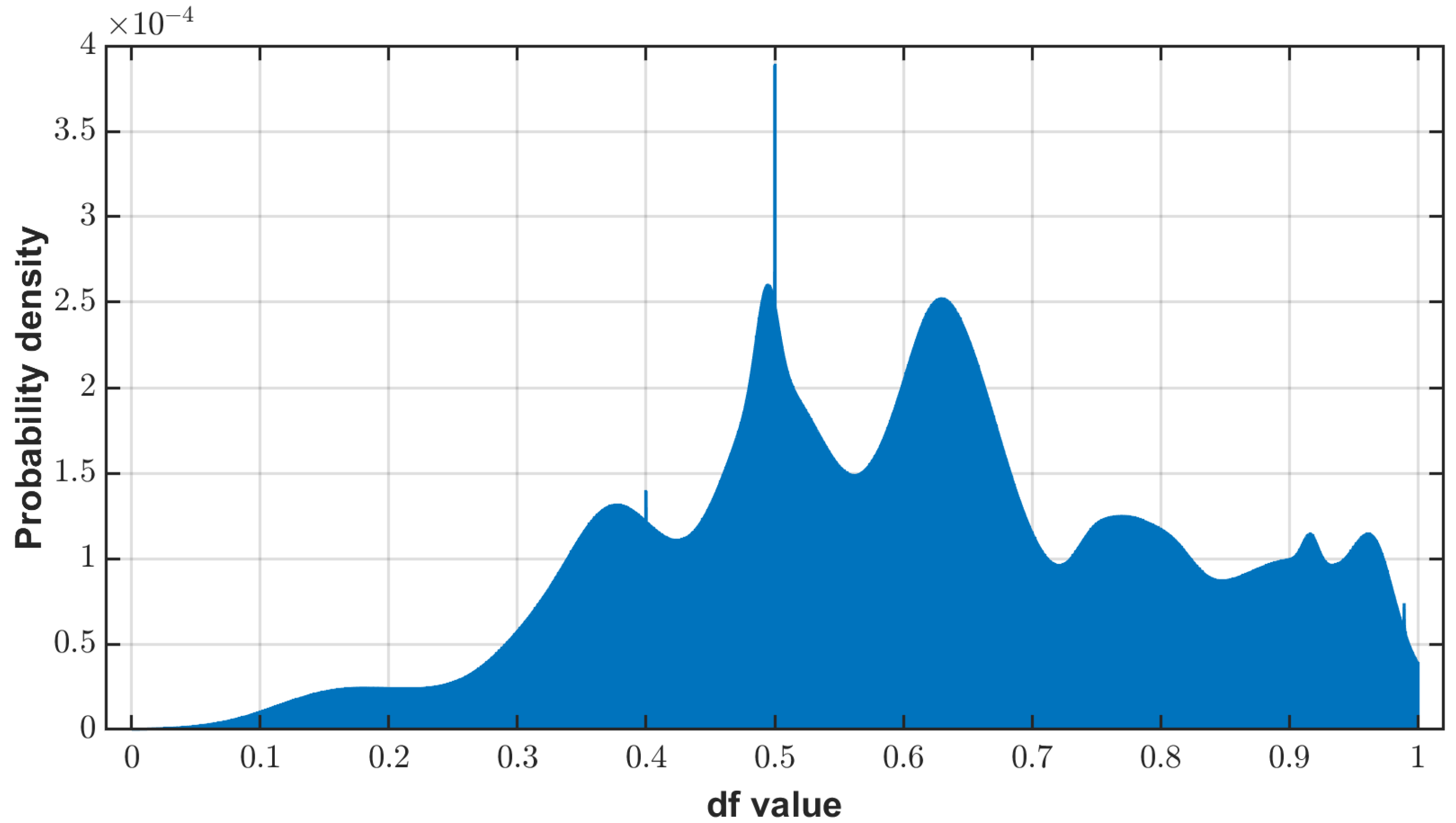
where the function $\mathsf{\Phi }$ is called the Decision Map—see Figure 3—and it estimates the probability density of all possible decisions based on the observations of the decisions made by participants. The probability density represents the relative commonality of each decision, i.e., a higher value of probability density means that the decision is made more commonly by the group of participants.

3.3. From HP to AP

In this section, we will discuss how human decisions are used as resources to establish new dimensions for encoding AP. Before we go into the details, an assumption has been made that in the group of participants there are some personality traits that may not be aligned with HP dimensions but are applicable for AP to encode individual differences in decision making. Meanwhile, the Decision Map provides a reference for assessing such differences, as it quantitatively captures the characteristics of commonality within this group of participants in the decision-making task. In the rest of this section, we will explain how the commonality information is extracted from the one-dimensional Decision Map and interpreted into multidimensional feature space, where individual decision sequences are distinguished and grouped as resources for encoding AP.

3.3.1. Two-Dimensional Commonality Interpretation

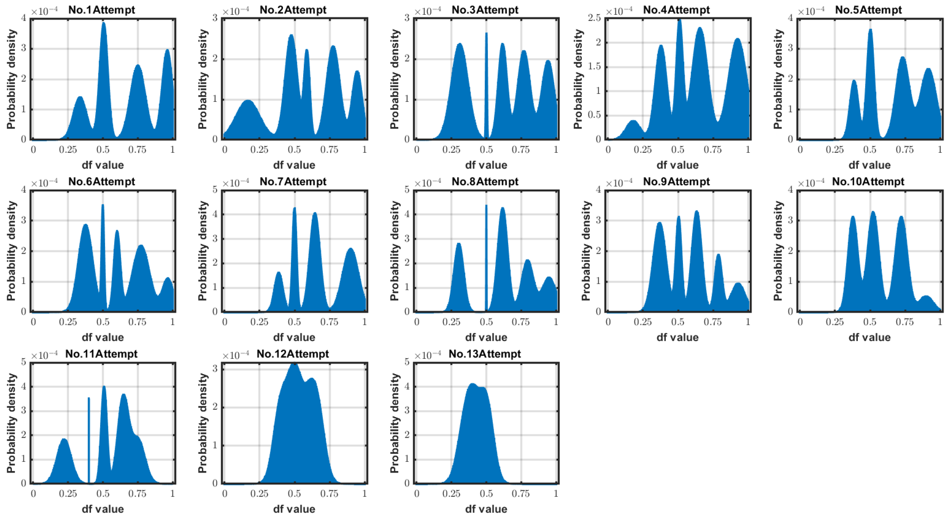
As a function, the Decision Map of $\mathsf{\Phi }\left(p_i^j\right)$ only measures the commonality of each decision without considering the factor of order in a decision sequence. To incorporate the ordinal factor, all decisions are divided into different subsets according to the order of attempts made by the participants. Regarding each order of attempt, a Decision Map is estimated, as shown in Figure 4.

Now, the commonality of each decision is measured in two dimensions: the order-free Decision Map denoted as $\theta ={\mathsf{\Phi }}_{OF}\left(p_i^j\right)$, and the order-related Decision Map denoted as $\mathsf{\zeta }={\mathsf{\Phi }}_{OR}\left(p_i^j\right)$. Thus, decisions are mapped from one-dimensional measurements to two-dimensional space as Figure 5a shows, and then they are classified into six clusters by the K-means method, as Figure 5b shows. In this process, decisions are clustered based on their commonality, which is measured by two dimensions corresponding to the order-free and order-related Decision Maps.

3.3.2. Decision Sequence in Multi-Dimensional Feature Space

As all decisions are clustered based on their commonality in the two-dimensional space, an individual decision sequence can be interpreted as picking decisions from different decision-commonality groups in the 2-D feature space. In this sense, we defined the feature space to represent the individual decision sequence. Feature space allows us to find clusters, patterns, and boundaries in the data. For example, algorithms such as k-means clustering or support vector machines (SVM) rely on distances and margins in this space to classify and group data. Feature space is a conceptual, multidimensional space where each dimension represents a particular feature (or attribute) of the data being analyzed. Defining a feature space based on the geometric representation of data involves selecting features that capture the shape, structure, and spatial relationships within the data. This approach is particularly useful when the data has a clear geometric or spatial structure, such as in computer vision, signal processing, and spatial analysis. When defining a feature space geometrically, the goal is to capture the intrinsic properties of the data that are relevant for the machine learning task. The extracted features in form of global and local geometrical vectors are explained as follows:

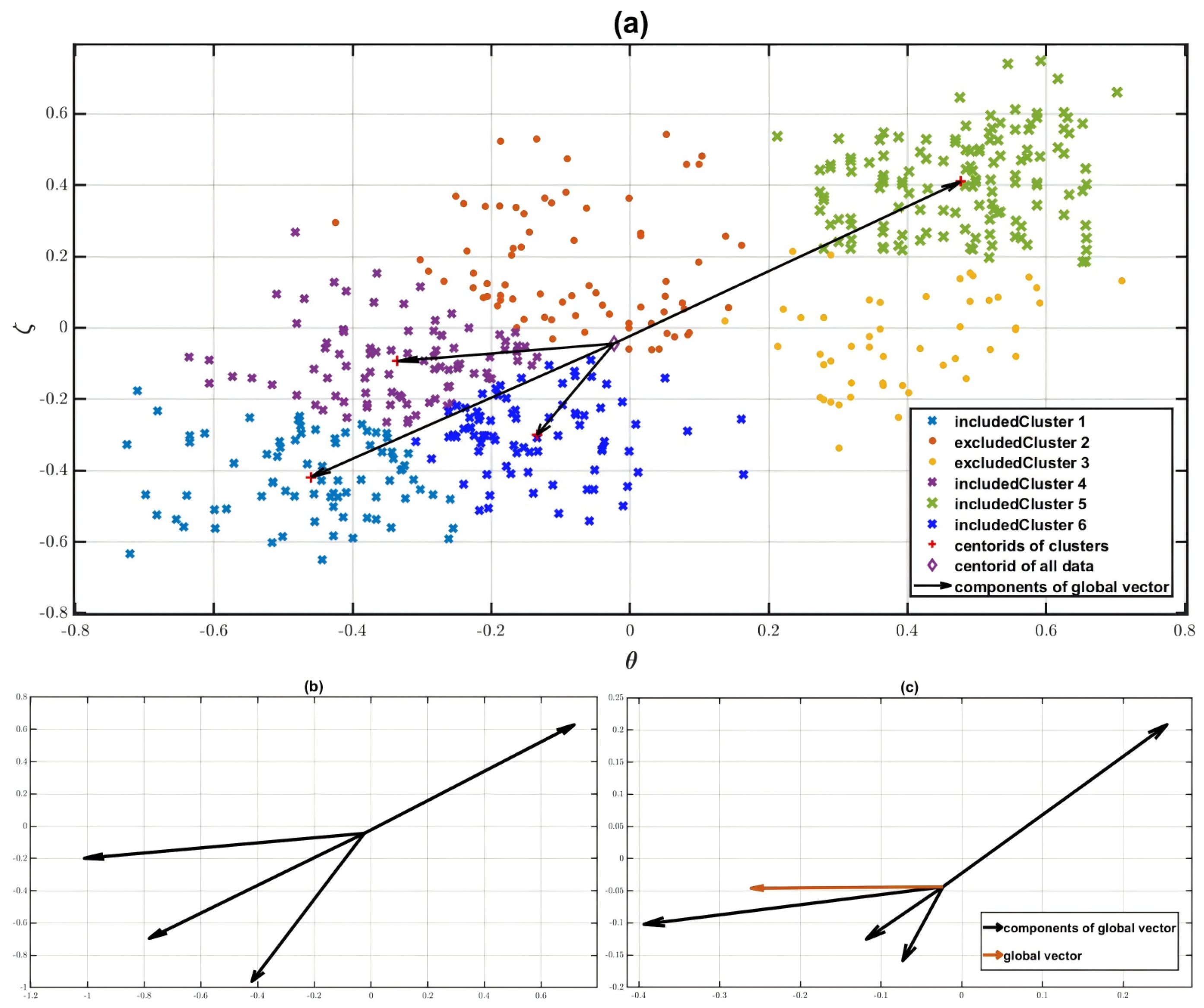
(1) Defining a global vector that contains the information on which decision-commonality group is included in a decision sequence. Figure 6 shows an example of a process for extracting global features. In the first step, as Figure 6a shows, the groups included in a decision sequence are identified by the vectors that range from the centroid of the entire dataset to each centroid of the cluster. In the second step, the identified vectors are normalized as unit vectors, as presented in Figure 6b. In the last step, all unit vectors are weighted according to the number of decisions incorporated into the corresponding group, and the global vector is identified by adding all the weighted vectors, as Figure 6c shows.

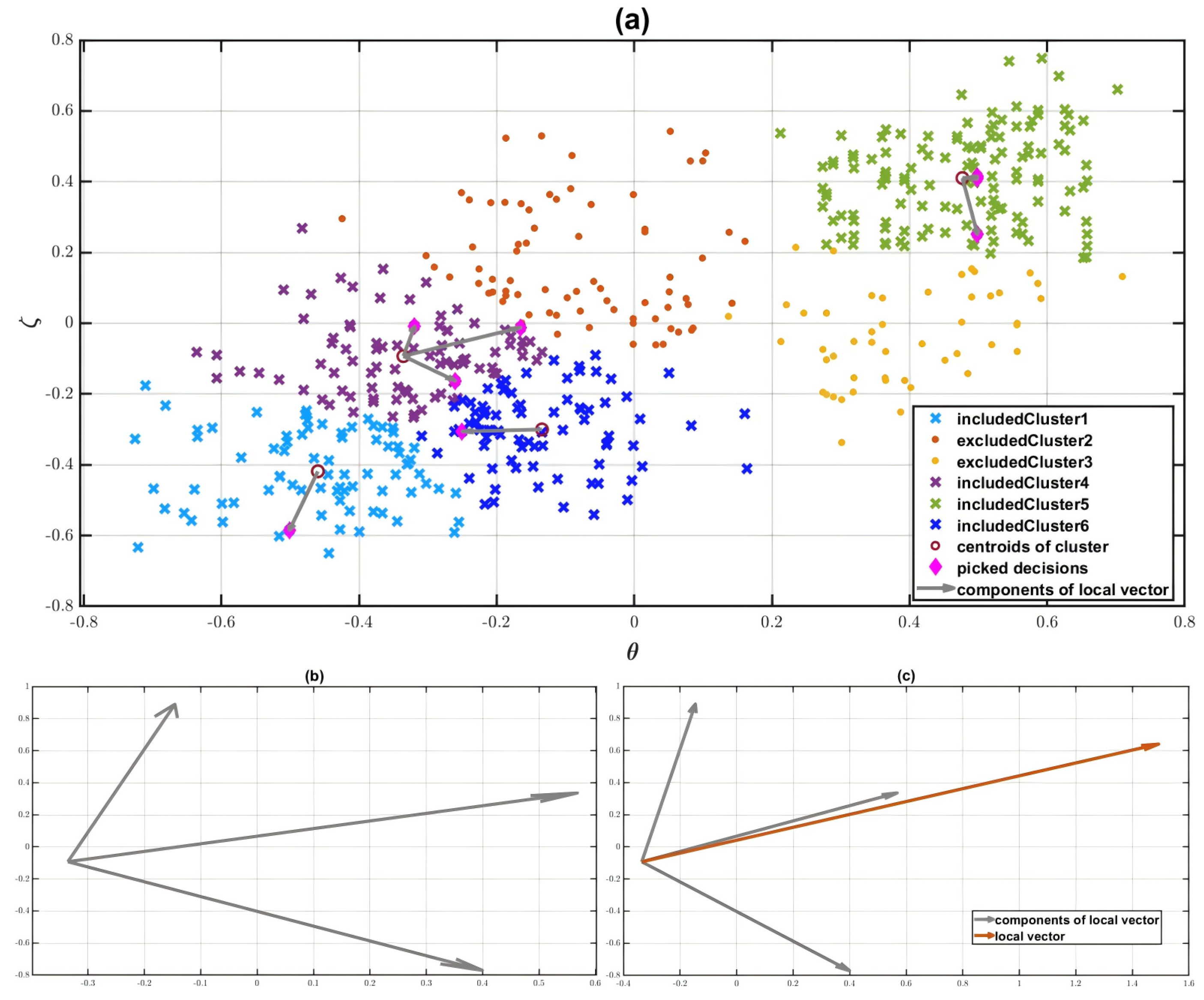
(2) Defining local vectors that contain information about individual decisions in each decision-commonality group. Figure 7 shows an example of the extraction of local features. In the first step, as Figure 7a shows, all decisions in a decision sequence are assigned to the corresponding clusters and identified by the vector from the centroid of the cluster to its own position within the cluster. In the second step, the identified vectors in each group are normalized as unit vectors, as presented in Figure 7b. In the last step, the local vector is identified by summing all unit vectors, as Figure 7c shows.

(3) The direction and magnitude of the identified vectors are extracted as global and local features to represent each decision sequence in the feature space.

Table 4. Examples of five decision sequences represented by extracted features.

Global Feature		Local Feature 1		Local Feature 2		Local Feature 3		Local Feature 4		Local Feature 5		Local Feature 6
$A_0$	$S_0$	$A_1$	$S_1$	$A_2$	$S_2$	$A_3$	$S_3$	$A_4$	$S_4$	$A_5$	$S_5$	$A_6$	$S_6$
197.97	0.13	36.76	0.11	312.39	0.19	139.32	0.04	139.64	0.20	347.22	0.13	102.49	0.20
156.18	0.15	27	0.29	330.22	0.62	249.15	0.28	327.02	0.27	0	0	81.88	0.56
123.73	0.21	273.86	0.23	305.98	0.14	98.06	0.14	95.93	0.15	357.21	0.33	148	0.17
198.66	0.14	7.68	0.13	19.14	0.35	238.95	0.05	259.69	0.28	0	0	90.52	0.08
67.09	0.13	343.93	0.18	0	0	269.83	0.13	186.18	0.55	226.09	0.48	0	0

presents the decision sequences of five participants that are represented by extracted features. Each row of the table indicates one decision sequence and each column indicates the extracted features, where the direction and magnitude of the global vector are, respectively, denoted as $A_0$ and $S_0$; the direction and magnitude of local vectors are, respectively, denoted from $A_1$ to $A_6$ and from $S_1$ to $S_6$, where the subscription stands for the index of the local vector.

3.3.3. Grouping Process

The grouping of participants can be achieved using the 1-D data of the Decision Map, 2-D data regarding the order-free and order-related commonality, or multidimensional features based on global and local vectors.

The commonality of participant’s decision sequence is quantified based on order-free and order-related Decision Map as follows:

$$x^j=\sum _{p_i^j\in d{f}^j}{\mathsf{\Phi }}_{OF}\left(p_i^j\right),$$

(7)

$$y^j=\sum _{p_i^j\in d{f}^j}{\mathsf{\Phi }}_{OR}\left(p_i^j\right),$$

(8)

where $d{f}^j$ is the decision sequence made by j participant. Equation (7) represents the 1-D data of the Decision Map; Equations (7) and (8) represent the 2-D data regarding decisions and the order of decisions; by mapping the 2-D data to global and local features, as mentioned in Section 3.2.2, a multidimensional feature space related to decisions and the order of decisions can be created.

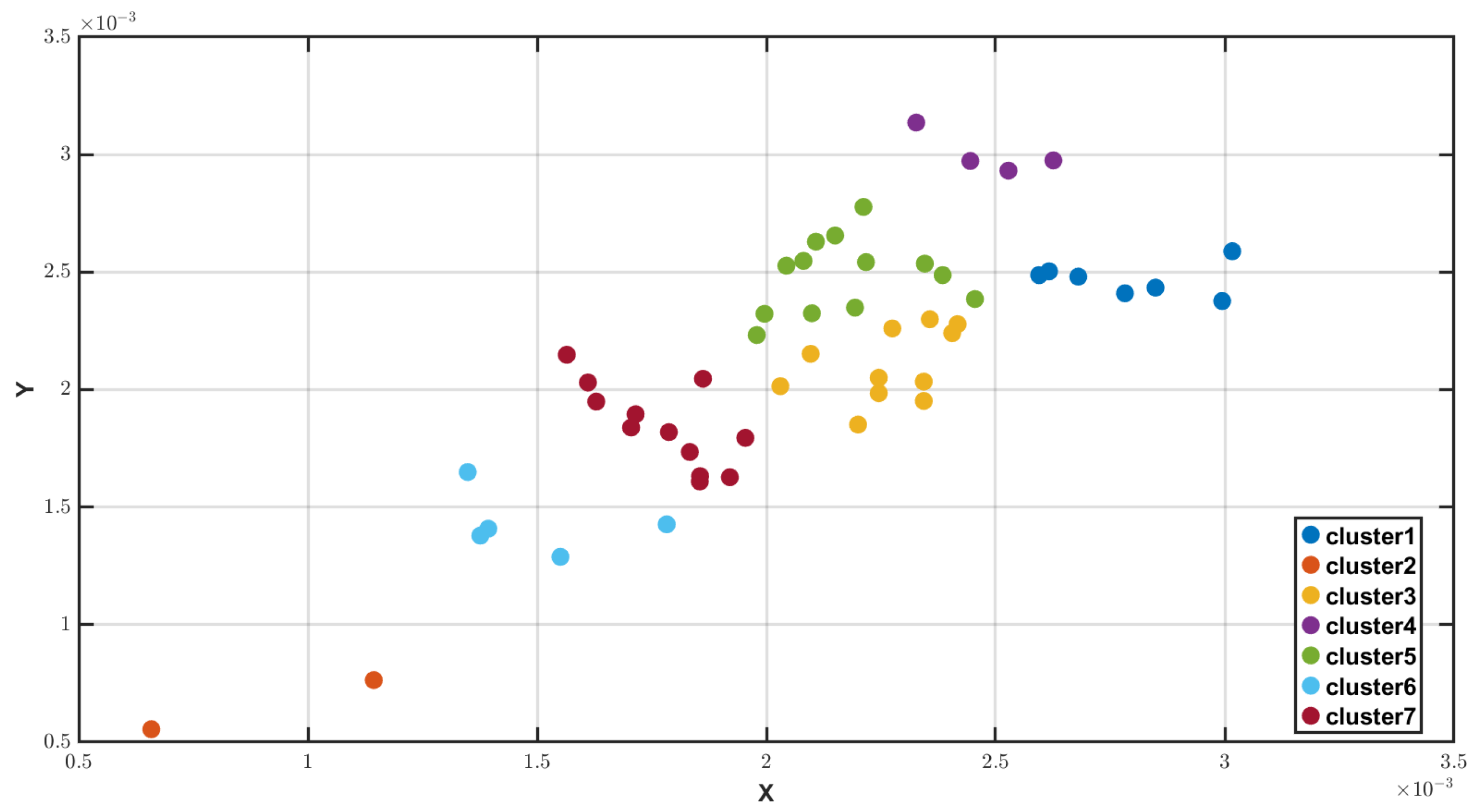
Using unsupervised machine learning algorithms such as k-means clustering, it is possible to construct participant groups by implementing 1-D or 2-D data in which each group shares some characteristic aspects; Figure 8 shows an example of grouping results of participants based on their decision sequence in 2-D space. However, both the 1-D and 2-D grouping suffer in terms of cluster stability (that is, the grouping result is significantly affected by the new data points). Introducing multiple features and mapping the 2-D data to the correspondent multiple feature space hypothetically can help in overcoming the instability, as this contributes to increasing the comparable information obtained from the features. In addition, the information introduced by the features should be independent of each other, which means that the multiple features should be orthogonal to each other. In our case the orthogonal feature space is created as follow:

$$D=X^T\beta +ϵ.$$

(9)

where X and D, including the extracted feature and 2D data distances, are as follows:

$$X=[A_0,S_0,A_1,S_1,A_2,S_2,\dots ,A_6,S_6],D=\left\{d^j\right\},$$

(10)

$$d^j=\sqrt{(x^{j2}+y^{j2})}.$$

(11)

The realization of the orthogonal feature space can be achieved by, for example, testing the model fit of a regression linear model.

Table 5. Feature-space orthogonality test.

	Estimate	SE	tStat	pValue
$ϵ$	3.00 $\times {10}^{-3}$	6.08 $\times {10}^{-5}$	49.78	6.56 $\times {10}^{-37}$
$A_0$	−6.87 $\times {10}^{-4}$	4.46 $\times {10}^{-4}$	−1.54	0.13
$s_0$	−1.21 $\times {10}^{-3}$	3.7 $\times {10}^{-5}$	−3.29	2.14 $\times {10}^{-4}$
$A_1$	6.29 $\times {10}^{-5}$	2.40 $\times {10}^{-4}$	0.26	0.80
$s_1$	3.05 $\times {10}^{-4}$	3.59 $\times {10}^{-4}$	0.85	0.40
$A_2$	1.67 $\times {10}^{-4}$	2.34 $\times {10}^{-4}$	0.71	0.48
$s_2$	4.09 $\times {10}^{-4}$	3.59 $\times {10}^{-4}$	1.14	0.26
$A_3$	4.65 $\times {10}^{-4}$	2.65 $\times {10}^{-4}$	1.76	0.09
$s_3$	2.77 $\times {10}^{-5}$	3.59 $\times {10}^{-4}$	0.08	0.94
$A_4$	−9.29 $\times {10}^{-5}$	2.20 $\times {10}^{-4}$	−0.42	0.68
$s_4$	9.25 $\times {10}^{-4}$	3.27 $\times {10}^{-4}$	2.82	7.40 $\times {10}^{-3}$
$A_5$	4.36 $\times {10}^{-4}$	2.80 $\times {10}^{-4}$	1.56	0.13
$s_5$	5.76 $\times {10}^{-4}$	3.53 $\times {10}^{-4}$	1.63	0.11
$A_6$	5.08 $\times {10}^{-6}$	3.25 $\times {10}^{-4}$	0.02	0.99
$s_6$	5.41 $\times {10}^{-4}$	3.81 $\times {10}^{-4}$	1.42	0.16

presents the result of such a test, modeling the features of all participants, where “Estimate” stands for the coefficient estimates of each term in the model; “SE” stands for the standard error of the estimated coefficients; “tStat” stands for the t-test for each coefficient which tests the null hypothesis (i.e., the corresponding coefficient is zero against the alternative hypothesis that it is different from zero); note that $tStat={\displaystyle \frac{Estimate}{SE}}$. Also, “pValue” stands for the p-value in the t-test of the two-sided hypothesis test; if a p-value is greater than 0.05, then the corresponding term is not significant at the $5\%$ significance level given the other term in the model. Therefore, orthogonal features are simply identified by p-values which are less than 0.05.

4. Results and Discussion

4.1. Orthogonal Features

In order to investigate how multiple features affect the grouping results in terms of variations and stability, the grouping process in multiple features, was performed with different feature spaces as follows:

$${\mathsf{\Omega }}_1=[A_0,S_0,A_1,S_1,A_2,S_2,\dots ,A_6,S_6];$$

$${\mathsf{\Omega }}_2=[S_0,N_0,S_1,N_1,S_2,N_2,\dots ,S_6,N_6];$$

$${\mathsf{\Omega }}_3=[A_0,S_0,N_0,A_1,S_1,N_1,S_2,N_2,\dots ,A_6,S_6,N_6];$$

$${\mathsf{\Omega }}_4=[S_1,S_2,S_3,\dots ,S_6],$$

where each space has a different setup of global and local features. In addition, a new set of parameters $\{N_0,N_1,\dots ,N_6\}$ was introduced in global and local features; $N_0$ represents the number of components in global vector, e.g., $N_0=3$ in Figure 7; $N_1$ to $N_6$ represent the number of components in the corresponding local vector, e.g., $N_4=3$ in Figure 8. In each feature space, the number of features included and their orthogonality are shown in

Table 6. Results of multiple-feature grouping process with different feature spaces.

Feature Space	Total Number of Features	Number of Orthogonal Features	Orthogonal Features
${\mathsf{\Omega }}_1$	14	4	[$S_0,S_3,S_5,A_6$]
${\mathsf{\Omega }}_2$	14	6	[$S_0,S_2,S_4,S_5,A_6,S_6$]
${\mathsf{\Omega }}_3$	21	7	[$N_0,N_2,S_3,N_3,A_4,N_4,N_5$]
${\mathsf{\Omega }}_4$	6	6	[$S_1,S_2,S_3,S_4,S_5,S_6$]

.

Each feature space provides different sets of orthogonal bases to measure the characteristic of participants in the decision-making process. In addition, changing the number of orthogonal features allows us to achieve different degrees of partitioning for the characteristics, as increasing the number of orthogonal features indicates that more information is needed to measure the decision-making characteristics. This argument is supported by the clustering results of participants based on their decision sequences, as shown by Figure 9. The mean number of clusters increases with increasing orthogonal features for all feature spaces, which allows us to determine the characteristics of the group of participants from more precisely from originally imprecise data.

4.2. Variation of Grouping

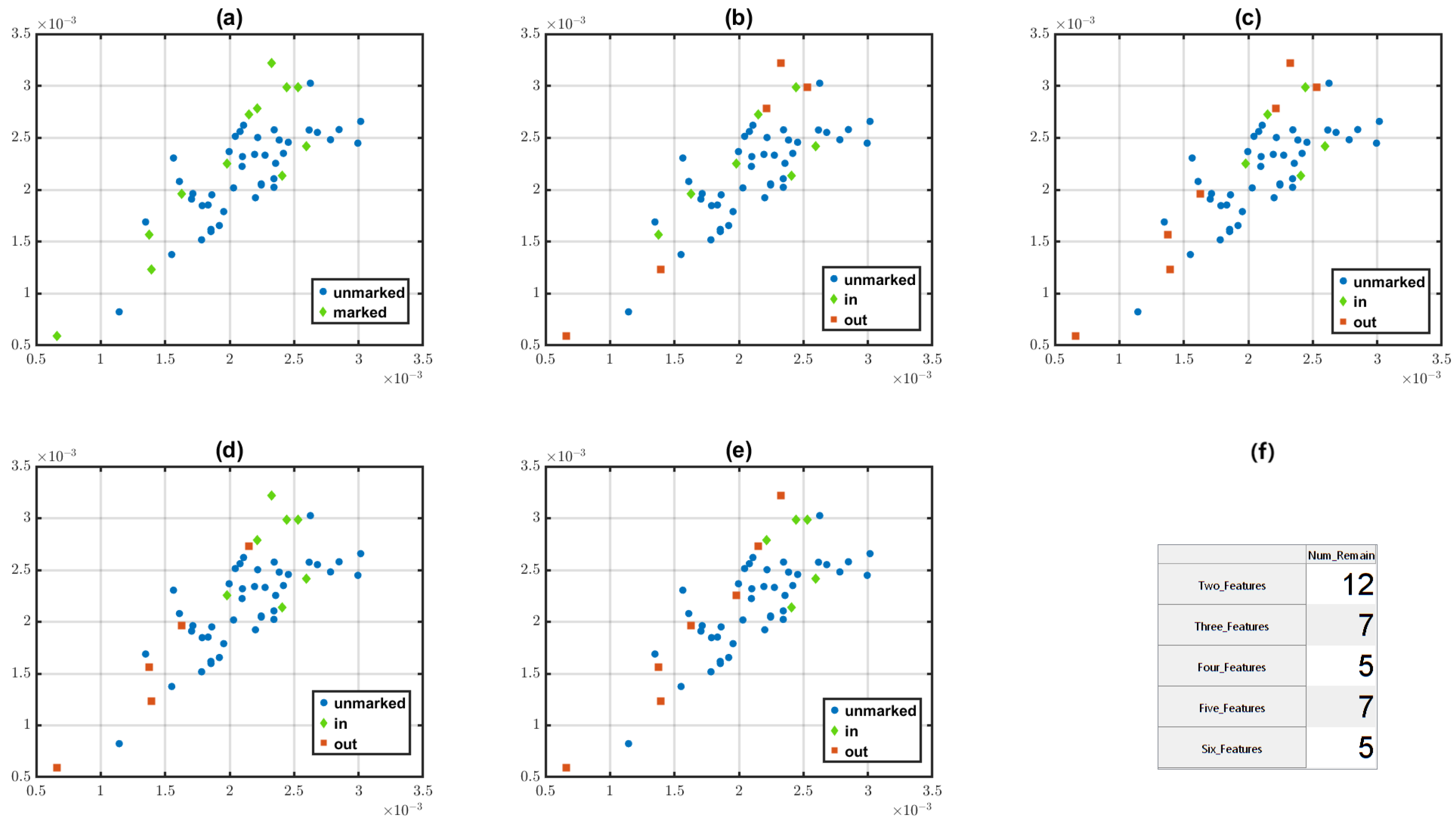
We evaluated the difference in membership by determining the different numbers of orthogonal features for grouping participants. Here, orthogonal features in space ${\mathsf{\Omega }}_4$ were used, as this space achieved a greater number of clusters on average (see Figure 9). The evaluation process is illustrated as follows: first, we randomly choose a participant and mark the same membership with two orthogonal features to delineate a group, as Figure 10a shows; then, we track the marked membership to see which members have different numbers of orthogonal features, as Figure 10b–e show; this random tracking is repeated B times in total, so the number of members remaining in the group with i number of orthogonal features after a repetition of b times is recorded as a set denoted $T^b=\left\{t_i^b\right\},i=2,3,4,5,6$; see Figure 10f. In this way, the set of differences in membership in terms of the number of features is denoted as $D_{ij}^B=\{t_i^b-t_j^b\},i>j$, $0<b<B$, where i and j represent different numbers of selected orthogonal features.

To examine the membership variations in partitions produced by numbers of orthogonal features, the random variable $D_{ij}^B$ is statistically investigated. Figure 11 presents histograms and fitted gamma distributions based on various subsets of $D_{ij}^B$. In Figure 11a–d, the subsets of $D_{ij}^B$ are collected cumulatively with increasing the number of orthogonal features from two to six, while in Figure 11d–g the subsets of $D_{ij}^B$ are collected stepwise. For all subsets of $D_{ij}^B$, the means are negative values, which indicates that the membership of the same group is separated after more characteristics (introduced by extra orthogonal features) are considered in the partition. However, subsets (d) to (g) show that the degree of this separation, the mean absolute value, is diminished after three orthogonal features were used for the partition; this also aligns with Figure 9, where the increasing rate for the mean number of clusters is reduced after three orthogonal features.

4.3. Grouping Stability

Although the orthogonal basis accounts for the characteristics of the participants that underlie their decision sequences, the use of these measures for clustering is still not validated for cluster quality. As a critical criterion, stability assesses the quality in terms of cluster reproducibility with perturbed versions of the original dataset [43]. One of the ways to generate perturbed data is the the bootstrap procedure [44], which resamples data with replacements, producing simulated datasets identical in size to the original. Thus, we resampled the original decision sequences of the participants (54 participants) at receptive sizes of $\{35,40,45,50\}$, and for each identical size, and the number of bootstrapping subsets is B, corresponding to the repetition times for random tracking in the last section. Then, we performed clustering with different numbers of orthogonal features based on each bootstrapping dataset (the same as that shown in Figure 10), and evaluated the reproducibility of clustering for the orthogonal basis from two perspectives, both the consistency of membership and the pattern of change in membership.

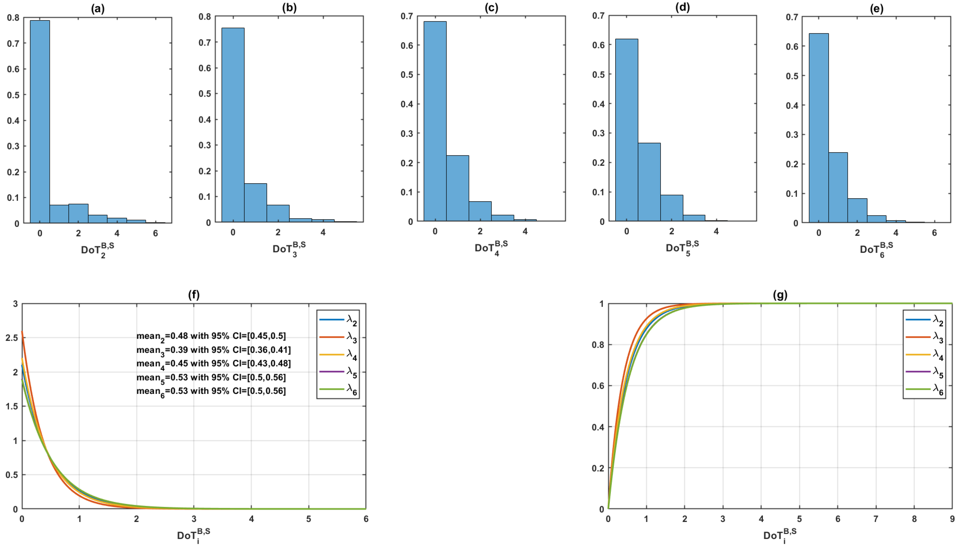
Regarding the consistency of membership, the marked members in the original data (as Figure 10a shows) is tracked during in the bootstrapped clusters, and the dissimilarity of the tracked memberships between the original and the bootstrapped cluster is denoted and calculated as follows: $Do{T}_i^{B,S}=\left\{\right|T_i^{B,54}-T_i^{B,S}\left|\right\},i=2,3,4,5,6$, $S=\{35,40,45,50\}$. As a random variable, the statistical results of $Do{T}_i^{B,S}$ are presented in Figure 12; subplots (a) to (e) show the histograms of $Do{T}_i^{B,S}$ regarding the number of orthogonal features that were used for clustering; in subplot (f), $Do{T}_i^{B,S}$ is fitted into the exponential distribution, where all estimated means (less than one) indicated that on average the dissimilarity between the bootstrap cluster and the original with orthogonal basis measurements is less than one membership (one element); the cumulative density function (CDF) in subplot (g) displays the estimated probability regarding the degree of dissimilarity with different numbers of orthogonal features, indicating that using three orthogonal features provide the most stability in clustering.

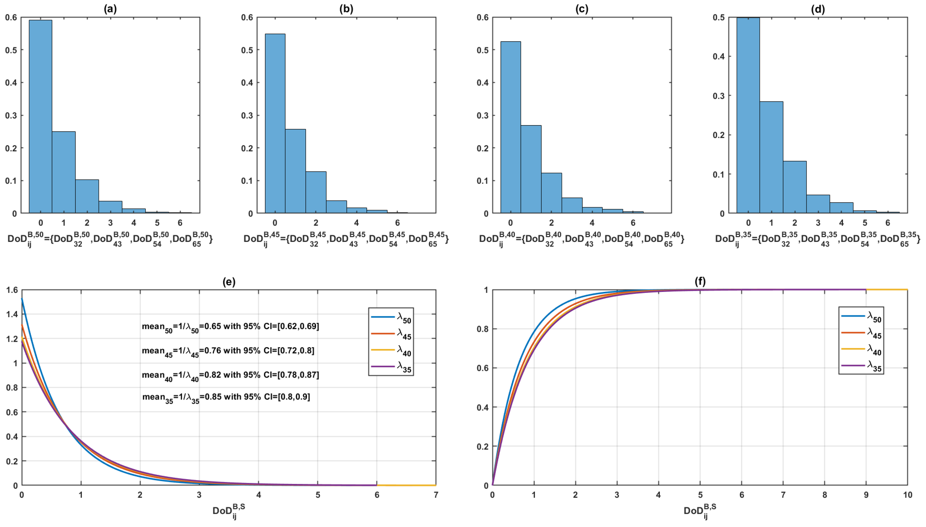
From another perspective, to evaluate cluster reproducibility, the pattern of change in membership caused by the number of orthogonal features during clustering is also tracked in the bootstrapped cluster, denoted as $D_{ij}^{B,S}$, where S represents the size of the bootstrapped data. Thus, the dissimilarity of this pattern between the bootstrapped cluster and the original cluster is denoted and calculated as follows: $Do{D}_{ij}^{B,S}=\left\{\right|D_{ij}^{B,54}-D_{ij}^{B,S}\left|\right\}$, $S=\{50,45,40,35\}$. The statistical results of $Do{D}_{ij}^{B,S}$ are presented in Figure 13; subplots (a) to (d) show the histograms of $Do{D}_{ij}^{B,S}$ regarding different sizes of bootstrapped datasets; in subplot (e), $Do{D}_{ij}^{B,S}$ is fitted into the exponential distribution as its histogram pattern, where all estimated means (less than one) indicated that, on average, the dissimilarity in membership changing between the bootstrapped cluster and the original cluster is less than one element; the cumulative density function (CDF) in subplot (f) displays the estimated probability regarding the degree of dissimilarity, indicating that the reproducibility for the pattern of changes in membership is reduced by shrinking the size of bootstrapped data resampled from the original.

The above results preliminarily show that the measures provided by orthogonal basis contribute to stability in terms of clustering individuals based on their decision sequences. However, this empirical evaluation is only performed by using a K-means algorithm, since the data measurement is focused on factors of cluster stability rather than clustering methods. A detailed study of implementing an orthogonal basis with multiple clustering methods to partition decisions is left for future work.

4.4. Grouping Result

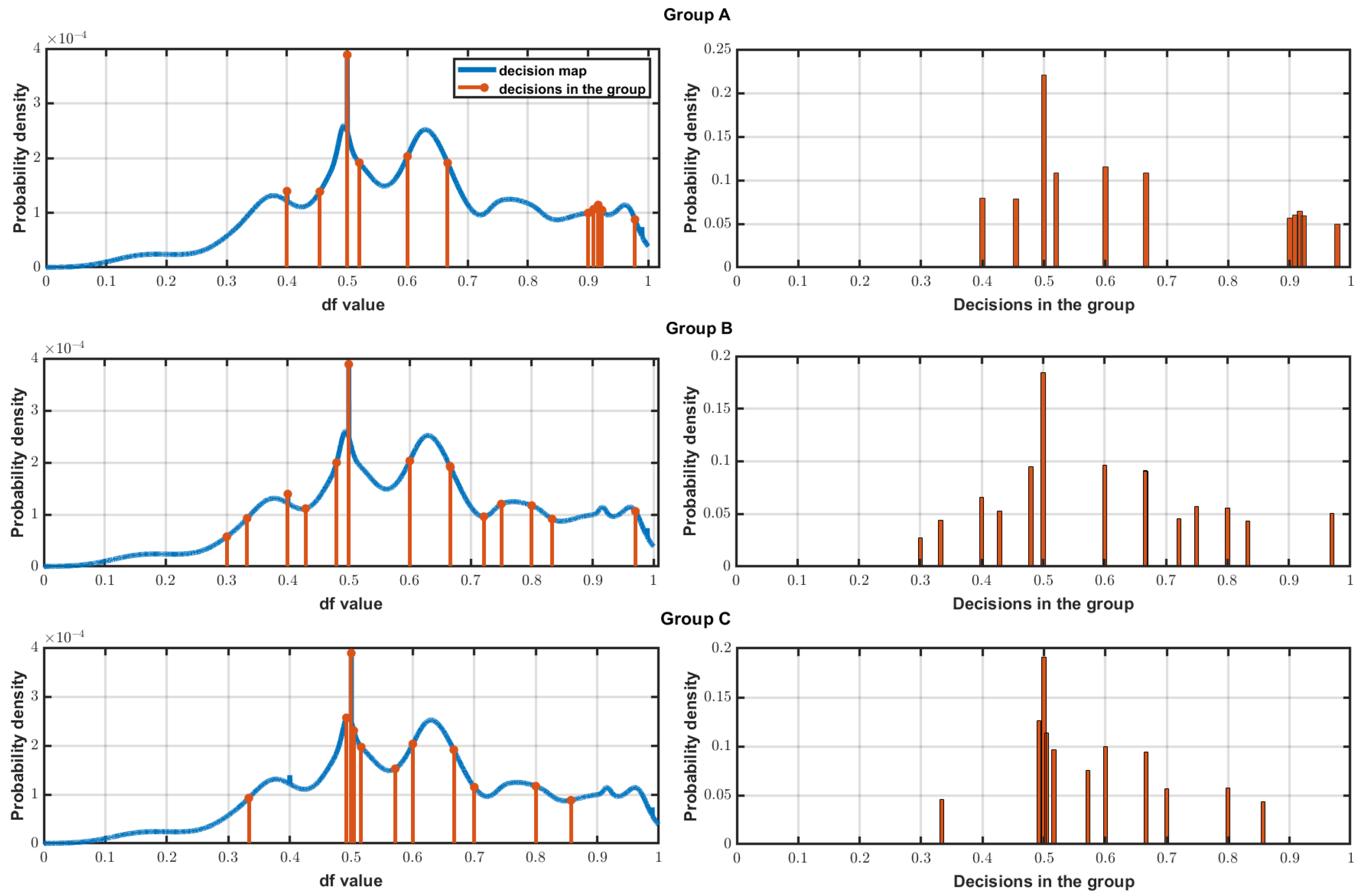
Individual decision sequences are distinguished and grouped with three orthogonal features, as they provide the most stability in the clustering test. Figure 14 shows three examples of grouping; commonalities are assigned to the grouped decisions by looking them up in the Decision Map, as shown on the left side, and then a probability mass function (PMF) is generated for each decision group by normalizing commonalities, as shown on the right side. The PMF of the decision will be interpreted as an individual characteristic for encoding AP, since it can provide distinct patterns of randomness for behavior generation.

4.5. Limitations and Future Plans

We believe we could show successfully how it is feasible to generate differentiable APs. In this respect, an intentionally designed low-level system complexity was used due to its simplicity and controllability to prove the feasibility of the proposed method, e.g., the use of a numerical guessing game with its low-level complexity level in decision making. This implies that the results are not proven to be valid for a more complex system, considering current assumptions, and cannot be directly extrapolated to real tasks with greater contextual, emotional richness, or interactions between agents. Another limitation of current work is related to not examining the cross-validation, e.g., if the obtained groupings are maintained or transformed when the type of task is changed, or elements of uncertainty or conflict are introduced to the system environment. We are aware of these typical limitations and plan further future work in this regard.

5. Conclusions

In this paper, we propose an approach to extract individual decision-making characteristics as a generative resource for encoding AP. The process of our approach is summarized as follows: (1) define a decision-making task where a group of participants’ decisions are collected and characterized by probability distribution, namely Decision Map, in which commonality in decisions is indicated by the probability density; (2) assume that some personality traits that do not align with HP model exist in participants and can be captured by the commonality in decisions made by participants; (3) generate order-related and order-free Decision Maps to measure the commonality of each decision with and without an ordinal factor in a decision sequence, and group all decisions in two-dimensional space according to their commonality measurements; (4) define feature spaces to represent decision sequences, then identify orthogonal features to distinguish decision sequences by group. The results show that different levels of discernibility can be achieved with different numbers of orthogonal features, but the discernibility is reduced after using three orthogonal features; As an initial step towards AP, the proposed approach investigated and built the casual relationship between personality and behavior through differentiating the characteristics of decision making. In future work, PMFs of APs can be used as a strategical model to generate action sequences for agents that can move with different random characteristics, representing the behavior of APs, with different dynamics such as stochastic process.

The relation of the proposed method and other works in areas such as imitation learning, affective computing, agent differentiation and reinforcement learning is presented in

Table 7. Comparisons between proposed methods and other methods.

Aspect	Imitation Learning [45]	Affective Computing [46]	Reinforcement Learning [47]	Agent Differentiation [48]	Our Proposed Method
Definition	Learning by mimicking human behavior from demonstrations	Computing systems that detect and respond to human emotions	Learning through trial and error to maximize long-term rewards	Categorizing agents based on their complexity, autonomy, and cognitive abilities	Learning strategical decision making from a group of people as a generative source for making differentiable APs
Core Focus	Replicating observed actions	Recognizing and responding to emotional states	Balancing exploration and exploitation for optimal decision making	Defining agent types based on goals, memory, learning and rationality	Generating differentiable APs
Learning Approach	Supervised, labeled expert demonstrations	Data-driven, often multimodal (facial expressions, voice, physiology)	Reward-based, often using deep learning	Varies from reflexive to cognitive agents	Unsupervised learning, non-Markovian as generative resource
Data Requirements	High-quality, context-rich demonstrations	Multimodal emotional data (speech, facial expressions, physiological signals)	Reward signals and state transitions	Varies, from simple rules to complex cognitive models	Decisions made in given context
Key Algorithms	Behavioral cloning, inverse reinforcement learning, GAIL	Emotion recognition models, sentiment analysis, speech emotion detection	Q-Learning, Deep Q-Networks, Actor-Critic Methods	Finite State Machines, Goal-based Agents, Utility-based Agents	Generative modelling in orthogonal space
Real-World Applications	Autonomous driving, humanoid robots, game AI	Emotional support systems, social robots, virtual assistants	Robotics, gaming, financial trading	Chatbots, industrial robots, personal assistants	Strategical navigation and steering in autonomous driving, strategical exploration and exploitation

in which the aspects of definition, core focus, learning approach, data requirements, key algorithms, and real-worlds applications are compared in summary.

Researchers from both technical and humanities fields emphasize the need to imbue Artificial Intelligence (AI) with human-like qualities, including self-awareness and free choice, raising critical questions about AI autonomy and control. Despite 20 years of work on the Artificial Personality project, the fundamental feasibility of creating an Artificial Personality remains unproven, with no single, widely accepted approach to its conceptualization and implementation. However, there are few current efforts such as [15] which are focusing on leveraging insights from studies of natural personality and intelligence to form a theoretical and methodological foundation for future AI personality projects. In this aspect we mentioned earlier that the key contribution of this paper is representing a meaningful step toward realizing the broader vision of artificial personality system by demonstrating the feasibility of developing distinct artificial personalities tailored to specific tasks. In our opinion a future possible way to solve the Artificial Personality project can be firstly to create a domain of agents having different tasks or even abstract of tasks and secondly based on this foundation find a theoretical framework for general APs.

References

1. Matthews, G.; Deary, I.J.; Whiteman, M.C. Personality Traits; Cambridge University Press: Cambridge, UK, 2003. [Google Scholar]
2. Roberts, B.W.; Yoon, H.J. Personality psychology. Annu. Rev. Psychol. 2022, 73, 489–516. [Google Scholar] [CrossRef]
3. Dhelim, S.; Aung, N.; Bouras, M.A.; Ning, H.; Cambria, E. A survey on personality-aware recommendation systems. Artif. Intell. Rev. 2022, 55, 2409–2454. [Google Scholar]
4. Tkalčič, M.; Chen, L. Personality and recommender systems. In Recommender Systems Handbook; Springer: New York, NY, USA, 2012; pp. 757–787. [Google Scholar]
5. Völkel, S.T.; Schödel, R.; Buschek, D.; Stachl, C.; Winterhalter, V.; Bühner, M.; Hussmann, H. Developing a personality model for speech-based conversational agents using the psycholexical approach. In Proceedings of the 2020 CHI Conference on Human Factors in Computing Systems, Honolulu, HI, USA, 25–30 April 2020; pp. 1–14. [Google Scholar]
6. Bouchet, F.; Sansonnet, J.P. Intelligent agents with personality: From adjectives to behavioral schemes. In Cognitively Informed Intelligent Interfaces: Systems Design and Development; IGI Global: Hershey, PA, USA, 2012; pp. 177–200. [Google Scholar]
7. Mou, Y.; Shi, C.; Shen, T.; Xu, K. A systematic review of the personality of robot: Mapping its conceptualization, operationalization, contextualization and effects. Int. J.-Hum.-Comput. Interact. 2020, 36, 591–605. [Google Scholar]
8. You, S.; Robert, L.P., Jr. Human-robot similarity and willingness to work with a robotic co-worker. In Proceedings of the 2018 ACM/IEEE International Conference on Human-Robot Interaction, Chicago, IL, USA, 5–8 March 2018; pp. 251–260. [Google Scholar]
9. Luo, L.; Ogawa, K.; Peebles, G.; Ishiguro, H. Towards a personality ai for robots: Potential colony capacity of a goal-shaped generative personality model when used for expressing personalities via non-verbal behaviour of humanoid robots. Front. Robot. AI 2022, 9, 728776. [Google Scholar]
10. Vinciarelli, A.; Mohammadi, G. A survey of personality computing. IEEE Trans. Affect. Comput. 2014, 5, 273–291. [Google Scholar] [CrossRef]
11. Chamorro-Premuzic, T. Personality and Individual Differences; John Wiley & Sons: Hoboken, NJ, USA, 2016. [Google Scholar]
12. Poulton, E.C. Behavioral Decision Theory: A New Approach; Cambridge University Press: Cambridge, UK, 1994. [Google Scholar]
13. Zhou, Y.; Khatibi, S. A New AI Approach by Acquisition of Characteristics in Human Decision-Making Process. Appl. Sci. 2024, 14, 5469. [Google Scholar] [CrossRef]
14. Mendelson, M.J.; Azabou, M.; Jacob, S.; Grissom, N.; Darrow, D.; Ebitz, B.; Herman, A.; Dyer, E.L. Learning signatures of decision making from many individuals playing the same game. In Proceedings of the 2023 11th International IEEE/EMBS Conference on Neural Engineering (NER), Baltimore, MD, USA, 24–27 April 2023; pp. 1–5. [Google Scholar]
15. Appelt, K.C.; Milch, K.F.; Handgraaf, M.J.; Weber, E.U. The Decision Making Individual Differences Inventory and guidelines for the study of individual differences in judgment and decision-making research. Judgm. Decis. Mak. 2011, 6, 252–262. [Google Scholar] [CrossRef]
16. Kostopoulos, G.; Davrazos, G.; Kotsiantis, S. Explainable Artificial Intelligence-Based Decision Support Systems: A Recent Review. Electronics 2024, 13, 2842. [Google Scholar] [CrossRef]
17. Ullah, A.; Mohmand, M.I.; Hussain, H.; Johar, S.; Khan, I.; Ahmad, S.; Mahmoud, H.A.; Huda, S. Customer analysis using machine learning-based classification algorithms for effective segmentation using recency, frequency, monetary, and time. Sensors 2023, 23, 3180. [Google Scholar] [CrossRef] [PubMed]
18. Alba, J.W.; Marmorstein, H. The effects of frequency knowledge on consumer decision making. J. Consum. Res. 1987, 14, 14–25. [Google Scholar] [CrossRef]
19. Ng, A.Y.; Russell, S. Algorithms for inverse reinforcement learning. In Proceedings of the Icml, Standord, CA, USA, 29 June–2 July 2000; Volume 1, p. 2. [Google Scholar]
20. Camerer, C.F.; Ho, T.H. Violations of the betweenness axiom and nonlinearity in probability. J. Risk Uncertain. 1994, 8, 167–196. [Google Scholar] [CrossRef]
21. Lin, J.; Keogh, E.; Lonardi, S.; Chiu, B. A symbolic representation of time series, with implications for streaming algorithms. In Proceedings of the 8th ACM SIGMOD Workshop on Research Issues in Data Mining and Knowledge Discovery, San Diego, CA, USA, 13 June 2003; pp. 2–11. [Google Scholar]
22. Cho, J.; Hyun, D.; Kang, S.; Yu, H. Learning heterogeneous temporal patterns of user preference for timely recommendation. In Proceedings of the Web Conference 2021, Ljubljana, Slovenia, 19–23 April 2021; pp. 1274–1283. [Google Scholar]
23. Pant, S.; Kumar, A.; Ram, M.; Klochkov, Y.; Sharma, H.K. Consistency indices in analytic hierarchy process: A review. Mathematics 2022, 10, 1206. [Google Scholar] [CrossRef]
24. Broekhuizen, H.; Groothuis-Oudshoorn, C.G.; van Til, J.A.; Hummel, J.M.; IJzerman, M.J. A review and classification of approaches for dealing with uncertainty in multi-criteria decision analysis for healthcare decisions. Pharmacoeconomics 2015, 33, 445–455. [Google Scholar] [PubMed]
25. Sahoo, S.K.; Goswami, S.S. A comprehensive review of multiple criteria decision-making (MCDM) Methods: Advancements, applications, and future directions. Decis. Mak. Adv. 2023, 1, 25–48. [Google Scholar] [CrossRef]
26. Elbanna, S.; Thanos, I.C.; Jansen, R.J. A literature review of the strategic decision-making context: A synthesis of previous mixed findings and an agenda for the way forward. M@n@gement 2020, 23, 42–60. [Google Scholar]
27. Hartley, C.A.; Phelps, E.A. Anxiety and decision-making. Biol. Psychiatry 2012, 72, 113–118. [Google Scholar] [CrossRef]
28. Deck, C.; Jahedi, S. The effect of cognitive load on economic decision making: A survey and new experiments. Eur. Econ. Rev. 2015, 78, 97–119. [Google Scholar] [CrossRef]
29. Chatzimparmpas, A.; Martins, R.M.; Kucher, K.; Kerren, A. Featureenvi: Visual analytics for feature engineering using stepwise selection and semi-automatic extraction approaches. IEEE Trans. Vis. Comput. Graph. 2022, 28, 1773–1791. [Google Scholar] [CrossRef] [PubMed]
30. Dunn, J.; Mingardi, L.; Zhuo, Y.D. Comparing interpretability and explainability for feature selection. arXiv 2021, arXiv:2105.05328. [Google Scholar]
31. Pyle, D. Data Preparation for Data Mining; Morgan Kaufmann: Burlington, MA, USA, 1999. [Google Scholar]
32. Cerda, P.; Varoquaux, G.; Kégl, B. Similarity encoding for learning with dirty categorical variables. Mach. Learn. 2018, 107, 1477–1494. [Google Scholar] [CrossRef]
33. Ravuri, A.; Vargas, F.; Lalchand, V.; Lawrence, N.D. Dimensionality Reduction as Probabilistic Inference. arXiv 2023, arXiv:2304.07658. [Google Scholar]
34. Younis, H.; Trust, P.; Minghim, R. Understanding High Dimensional Spaces through Visual Means Employing Multidimensional Projections. arXiv 2022, arXiv:2207.10800. [Google Scholar] [CrossRef]
35. Xiao, Z.; Xu, X.; Xing, H.; Luo, S.; Dai, P.; Zhan, D. RTFN: A robust temporal feature network for time series classification. Inf. Sci. 2021, 571, 65–86. [Google Scholar] [CrossRef]
36. Zhang, R.; Hao, Y. Time Series Prediction Based on Multi-Scale Feature Extraction. Mathematics 2024, 12, 973. [Google Scholar] [CrossRef]
37. Leão, C.P.; Carneiro, M.; Silva, P.; Loureiro, I.; Costa, N. Decoding the Effect of Descriptive Statistics on Informed Decision-Making. In Proceedings of the International Conference Innovation in Engineering, Nagoya, Japan, 16–18 August 2024; Springer: Cham, Switzerland, 2024; pp. 135–145. [Google Scholar]
38. Devore, J.L.; Berk, K.N.; Carlton, M.A. Overview and descriptive statistics. In Modern Mathematical Statistics with Applications; Springer: Cham, Switzerland, 2021; pp. 1–48. [Google Scholar]
39. Mazumdar, N.; Sarma, P.K.D. Sequential pattern mining algorithms and their applications: A technical review. Int. J. Data Sci. Anal. 2024. [Google Scholar] [CrossRef]
40. Hosseininasab, A.; van Hoeve, W.J.; Cire, A.A. Constraint-based sequential pattern mining with decision diagrams. In Proceedings of the AAAI Conference on Artificial Intelligence, Honolulu, HI, USA, 27 January–1 February 2019; Volume 33, pp. 1495–1502. [Google Scholar]
41. Nguyen, T.N.; Jamale, K.; Gonzalez, C. Predicting and Understanding Human Action Decisions: Insights from Large Language Models and Cognitive Instance-Based Learning. In Proceedings of the AAAI Conference on Human Computation and Crowdsourcing, Pittsburgh, PA, USA, 16–19 October 2024; Volume 12, pp. 126–136. [Google Scholar]
42. Sun, X.; Li, X.; Zhang, S.; Wang, S.; Wu, F.; Li, J.; Zhang, T.; Wang, G. Sentiment analysis through llm negotiations. arXiv 2023, arXiv:2311.01876. [Google Scholar]
43. Liu, T.; Yu, H.; Blair, R.H. Stability estimation for unsupervised clustering: A review. Wiley Interdiscip. Rev. Comput. Stat. 2022, 14, e1575. [Google Scholar] [CrossRef] [PubMed]
44. Beran, R. An introduction to the bootstrap. In The Science of Bradley Efron; Springer: Berlin/Heidelberg, Germany, 2008; pp. 288–294. [Google Scholar]
45. Hussein, A.; Gaber, M.M.; Elyan, E.; Jayne, C. Imitation learning: A survey of learning methods. ACM Comput. Surv. (CSUR) 2017, 50, 1–35. [Google Scholar]
46. Pei, G.; Li, H.; Lu, Y.; Wang, Y.; Hua, S.; Li, T. Affective computing: Recent advances, challenges, and future trends. Intell. Comput. 2024, 3, 0076. [Google Scholar] [CrossRef]
47. Wang, X.; Wang, S.; Liang, X.; Zhao, D.; Huang, J.; Xu, X.; Dai, B.; Miao, Q. Deep reinforcement learning: A survey. IEEE Trans. Neural Netw. Learn. Syst. 2022, 35, 5064–5078. [Google Scholar] [CrossRef]
48. Zhong, Y.; Kuba, J.G.; Feng, X.; Hu, S.; Ji, J.; Yang, Y. Heterogeneous-agent reinforcement learning. J. Mach. Learn. Res. 2024, 25, 1–67. [Google Scholar]
Figure 1. A flowchart of the number-guessing game.
Ai 06 00184 g001
Figure 2. Examples of decision clustering results, (a,b) present two participants’ decisions (df value) and their respective clustering results.
Ai 06 00184 g002
Figure 3. The Decision Map of a group of people.
Ai 06 00184 g003
Figure 4. Decision Maps of all participants, with consideration of attempt order.
Ai 06 00184 g004
Figure 5. (a) An interpretation of all decisions in terms of 2-D measurements, for both order-free and order-related commonality. (b) Decision-commonality groups in 2-D feature space by using K-means clustering method.
Ai 06 00184 g005
Figure 6. An example of defining the global vector for a decision sequence. (a) the included decision groups (cluster 1, 4, 5 and 6) are represented by vectors from the centroid of all data (diamond mark) to the centroids of corresponding cluster (plus marks); (b) these vectors are normalized in unit vectors; (c) the unit vectors are weighted by the number of decisions in the corresponding group, and addition of weighted vectors defines the global vector (orange-color vector) for current decision sequence.
Ai 06 00184 g006
Figure 7. An example of defining the local vectors for a decision sequence. (a) in each decision groups (cluster 1, 4, 5 and 6), the included decisions are represented by vectors from the centroids of cluster (circle marks) to corresponding positions (pink diamond marks); (b) the identified vectors in cluster 4 are presented and they are normalized in unit vectors; (c) the addition of unit vectors defines the local vector (orange-color vector) within a decision group.
Ai 06 00184 g007
Figure 8. Grouping result of participants based on their 2-D data, x j and y j .
Ai 06 00184 g008
Figure 9. Clustering results of the decision sequence represented by different feature spaces.
Ai 06 00184 g009
Figure 10. Visualization of tracking membership in partitions with different numbers of orthogonal features. Each point in the subplots represents a participant (same as in Figure 8). (a) When two orthogonal features are used for partition, a random participant and her/his members are marked; (be) show increases in the number of orthogonal features from three to six, tracking the membership in the partition by using a green diamond and a red square to mark in and out, respectively; (f) the number of members remaining in this random tracking b is recorded as a set T b = { t 2 b = 12 , t 3 b = 7 , t 4 b = 5 , t 5 b = 7 , x 6 b = 5 } .
Ai 06 00184 g010
Figure 11. Variations in membership difference in partitions. The histograms depict subsets of D i j B , (ag), where B = 300 , i = 3 , 4 , 5 , 6 , j = 2 , 3 , 4 , 5 , and i > j . The orange curves depict left-skew (flipped) gamma distributions which are estimated based on the subsets of D i j B ; the shape parameter α and the rate parameter β are estimated for right-skew gamma distribution, while the mean and variance of D i j B are estimated after flipping. The details of the collections in the subset are shown on the label along the horizontal axis.
Ai 06 00184 g011
Figure 12. The reproducibility of the clustering analysis based on cluster membership; (ae) display the histograms based on subsets of D o T i B , S , where B = 300 , S = 35 , 40 , 45 , 50 , i = 2 , 3 , 4 , 5 , 6 ; (f) according to the pattern of histogram, the exponential distribution is estimated based on each subset of D o T i B , S , and the estimated means and their 95% confidence intervals are displayed; (g) the CDF of each distribution indicates the degree of dissimilarity regarding different numbers of orthogonal features.
Ai 06 00184 g012
Figure 13. The reproducibility of the clustering analysis based on the pattern of change in membership; (ad) display the histograms based on subsets of D o D i j B , S , where B = 300 , S = 35 , 40 , 45 , 50 , i = 3 , 4 , 5 , 6 , j = 2 , 3 , 4 , 5 , and i > j ; (e) according to the pattern of the histogram, the exponential distributions is estimated for subsets of D o D i j B , S , and the estimated means and their 95% confidence intervals are displayed; (f) the CDF of each distribution indicates the degree of dissimilarity regarding different sizes of bootstrapped datasets.
Ai 06 00184 g013
Figure 14. Three examples of grouped decision sequences. The left-side subplots show the relative commonalities of individual decisions in the grouped sequences, determined by looking them up in the Decision Map. The right-side subplots show the probability mass functions of individual decisions in the grouped decision sequences by normalizing their commonalities.
Ai 06 00184 g014