Abstract
Occupancy detection for large buildings enables optimised control of indoor systems based on occupant presence, reducing the energy costs of heating and cooling. Through machine learning models, occupancy detection is achieved with an accuracy of over 95%. However, to achieve this, large amounts of data are collected with little consideration of which of the collected data are most useful to the task. This paper demonstrates methods to identify if data may be removed from the imbalanced time-series training datasets to optimise the training process and model performance. It also describes how the calculation of the class density of a dataset may be used to identify if a dataset is applicable for data reduction, and how dataset fusion may be used to combine occupancy datasets. The results show that over 50% of a training dataset may be removed from imbalanced datasets while maintaining performance, reducing training time and energy cost by over 40%. This indicates that a data-centric approach to developing artificial intelligence applications is as important as selecting the best model.
1. Introduction
Indoor occupancy detection is an important task for operations such as energy saving, management, and security [1,2]. It allows for automated control of heating, ventilation and air conditioning (HVAC) by only powering these systems when occupant presence is detected. A classic approach to occupancy detection for indoor environments is to deploy multiple homogeneous sensors, which are positioned around the interior for maximum coverage, and feed these data into an artificial intelligence (AI) model. These sensors collect thousands of datapoints each day, resulting in copious datasets which require processing, cleaning, and validating before they can be used to estimate occupancy. To coalesce these data from multiple sources, embedded or “edge” devices are ideal due to their small size and ease of use. Edge devices are low-power and low-compute devices, making them appropriate for energy-saving solutions, but this makes them incapable of running the increasingly complex AI models that have become commonplace. Cloud computing allows these devices to send data to a more powerful machine for classification, but data transmission has a high energy cost, especially when large amounts of data must be sent multiple times a minute [3]. To alleviate this cost, it is beneficial to perform as much processing as early in the pipeline as possible on the edge device and reduce the amount of data to be sent. In order to optimise these devices for use on such large collections of data, data analysis can give us an understanding of which data are more or less relevant to the task at hand, and therefore, which data may be removed from the training dataset. This can minimise the amount of data transmitted further and stored. Additionally, environmental datasets often suffer from noise and class imbalance which can lead to bias in training [4,5]. By reducing the amount of data in the majority class, class balance may be alleviated and the cost of transmission reduced. This paper aims to show that, depending on the attributes of the data, derived from centroid distance and class density, some data may be removed and model performance maintained. It also aims to find the compatibility of low-compute Random Forest (RF) algorithms with data reduction to maximise data efficiency. The final aim is to perform dataset fusion on occupancy datasets to observe if previously obtained data may be used with newly collected data for a more robust classifier. The experimentation includes reduction strategies inspired by previous works on image data to identify compatibility of these methods with lower-dimensional environmental sensor data.
1.1. Related Works
This paper discusses three topics: Data reduction to find the most useful data in the time-series domain, machine learning for occupancy detection, and dataset fusion of time-series data.
With the rapid expansion of AI, the models and data necessary for its operation have grown substantially, posing sustainability challenges for users [6]. Also, the environmental effects of AI have become an increasing concern, leading to the trend towards green AI [7]. For these reasons, there is a strong desire to be able to train AI more cheaply. This includes both more efficient AI models and training data. Generally, an increase in data can enhance model performance; however, recent research has focused on identifying the most useful data to streamline collection efforts and model training [8]. This targeted approach reduces the resources required for training without sacrificing accuracy or performance.
Class imbalance can lead to bias, where the model favours a class’s samples due to its larger sample size. To counter this, imbalance can be relieved by adding artificial samples to the smaller (minority) class, or removing samples from the larger (majority) class. These processes are called undersampling and oversampling, respectively [9]. Undersampling can be considered a data reduction technique as it reduces the size of the dataset.
Data pruning [10] is a technique that reduces an entire dataset by giving each datapoint a ‘parameter influence’, and then removing datapoints with the lowest influence. In this way, not only is data utility optimised but also the computational load of training the model. A similar alternative is to perform preliminary training for a few iterations on a complete dataset to first identify the most impactful features. After these features are identified, only they are used to train for the full duration [11]. Research by Toneva et al. [12] used the ‘forgetting score’ as a metric to group data, eliminating less forgotten and therefore less useful data before training on the refined dataset. This practice further minimises time and computational resources, increasing overall efficiency.
Dimensionality reduction is a popular technique which transforms data into a lower-dimensional space. This reduction aids in data visualization and addresses challenges associated with the ‘curse of dimensionality’, which can impede data grouping and analysis [13]. Principal component analysis (PCA), for example, identifies and analyses principle components within a dataset, which may then be used as feature sets for training, replacing raw data [14]. By using only these essential components, models experience a reduction in complexity and operational costs without sacrificing key data insights or performance. Dimensionality reduction is popular in reducing image data [15], but when reducing time-series data it is important to consider the temporal nature of the data, and that feature order must be preserved. PCA has proven to be useful as a preprocessing step before applying machine learning, but assumes linearity in the data. Kernel PCA (KPCA) resolves this by applying a kernel to the data, allowing it to handle non-linearity, but it has a high computational overhead [16].
Understanding the most useful data in a dataset is important, but it is also important to understand which data are most useful at different stages of training. Usually, training AI models involves several iterations of computation on the full dataset. However, recent work on dynamic data inclusion shows an alternative in which a model is trained for some time on a subset of the data, and gradually data exposure is increased over time [17]. After identifying which data are ‘easy’ to learn and which are ‘hard’, by means of parameter influence or the forgetting score, training may be performed with only the easier data for more rapid training, and fine-tuned with harder data once the model parameters have been improved.
Many of these methods produce a data subset which is used for partial training. While this is an improvement from training on a full dataset, there is a desire to be able to identify the usefulness of data without having to use AI at all. The work in [18] aims to identify redundant data in a dataset, which may be removed from training before running any AI models at all. By calculating the ‘class density’, each class is given a score which may be used to quantify how much data may be removed before training.
Occupancy detection using AI holds significant potential for optimizing heating, ventilation, and air conditioning (HVAC) systems to achieve greater energy efficiency and cost savings [19,20]. While methods such as camera-based systems can be employed to detect occupancy, these techniques are often seen as intrusive by users, as they may infringe on privacy and personal comfort [21,22]. To address these concerns, non-intrusive sensing methods are preferred. These alternatives rely on environmental indicators like temperature, humidity, and CO2 levels within a space to infer human presence. Such non-intrusive techniques offer a viable solution for occupancy detection, achieving notable success while preserving user privacy [21,23].
AI models are most often trained on data specific to the domain they are to operate in. However, data from the real world may be combined to make it more heterogeneous and informative, increasing the reliability of the classification and quality of the extracted information [24]. ‘Data fusion’ refers to the combination of multiple features into a single dataset, which is used in regression or classification [25]. In the context of occupancy detection, this is often referred to as sensor fusion, as multiple sensor readings are concatenated into one complete dataset. ‘Dataset fusion’ allows AI models to perform more reliably in new domains by introducing data from multiple sources. By combining datasets, information from other domains becomes available, giving improved performance when tested in other domains. This is a popular method in image classification tasks, as new images are easily resized to match the original data [26]. However, time-series datasets are seldom in the same format as each other, due to the domain-specific information they capture. This is true even for datasets that aim to capture the same information; for example, in the case of occupancy detection, occupancy datasets capture different types of data such as temperature and humidity, image and sound, altitude and location. When attempting to fuse these datasets, this causes issues such as mismatching data formats or missing data, which makes training difficult. Data pre-processing must be performed in order to homogenise datasets prior to fusion. There has been less attention given to fusing completed occupancy datasets together to improve model robustness.
1.2. Research Gap and Contributions
There has been recent research on data reduction for time-series data, but not on occupancy data specifically. Moreover, there is a research gap in fusing occupancy datasets. To address this, this paper describes data reduction techniques, based on previous work on image datasets, developed for time-series data. More specifically, these techniques focus on sorting time-series data by their distance from the data centroid, and reduction is performed based on this metric.
This paper aims to show the effects of data reduction in two aspects: reduction across all classes indiscriminately, and reduction of only the larger class. This comparison will show if undersampling is better than pure, random data reduction in the context of occupancy data. Also, this paper investigates the effects of varying amounts of data reduction to observe the optimal amount of reduction for best performance. This paper aims to then correlate these findings with class density, to observe if this technique is applicable to time-series data, where it has previously only been tested on high-dimensionality image datasets. Finally, this paper demonstrates the effectiveness of data reduction techniques on individual datasets and fused datasets to identify the suitability of data reduction on one-dimensional data.
We define the most useful data as the data that best describe a model, while the least useful data are those which do not provide any new information to the model. We define sufficient data as the amount of data required to successfully train an AI model. By identifying the sufficient amount of data, it is possible to optimise training by not spending resources training on data that do not contribute further to model performance.
Our contributions are as follows:
- This paper introduces methods of data reduction for time-series data based on previously established techniques for 2D image data;
- This paper shows, through experimentation, the benefits and drawbacks of varying amounts of data reduction on time-series data;
- This paper compares data reduction on the larger of imbalanced classes and data reduction on the entire dataset to identify the effects of data undersampling in conjunction with our novel data reduction strategies;
- This paper shows the correlation between class density and model and model performance after data reduction to show how data reduction may be suitable for a given dataset;
- This paper shows the suitability of dataset fusion for occupancy datasets, in combination with data reduction.
2. Materials and Methods
We aim to identify the most useful data in a dataset. We achieve this by calculating centroid distances, which consolidate all the features, the sensor values, into one variable. This allows data to be organised by a single metric, which is used to remove data by our multiple data reduction techniques, giving us reduced datasets. These reduced datasets are used for training and testing, and the results are compared to show which data reduction method, and therefore which data, is most beneficial for training. However, as occupancy data commonly have an imbalanced number of datapoints in each class, we propose a method of balancing data by removing data from only the larger class. This resolves both issues of class imbalance and the abundance of less useful data.
2.1. Dataset Preparation and Fusion
Multiple open-source datasets have been developed for the purpose of occupancy detection with machine learning [27,28]. The dataset selected for this experiment is the HPDMobile dataset [29], due to it having multiple sites of homogeneous environmental sensor data, making it ideal for dataset fusion. It is an open-source dataset that collects data from six sites, with each site containing the same type of sensors and using the same capture methods. Each sensor device captures temperature, humidity, and the volatile organic compound (VOC) count. Each site has either four or five of these sensors, which equates to twelve or fifteen features for each site, respectively. Each datapoint has an associated ground truth of the number of occupants, but for the sake of simplicity, the experimentation aims to differentiate between ‘some’ or ‘no’ occupants.
The HPDMobile dataset is not originally formatted by site, but by sensor; each sensor’s data are stored in a separate file. To make a complete dataset, each file of sensor data is sorted by location, time, and date and aggregated into a table for each site. The result is a dataset csv file for each of the six sites. Details of the six subsets of the HPDMobile dataset are shown in Table 1.

Table 1.
HPDMobile dataset information. Class balance ratio is between classes ‘Not Occupied’ and ‘Occupied’. Each sensor contains three features: temperature, humidity, and VOC.
The HPDMobile dataset has on average 7% of data missing across all sites and time frames due to sensor synchronisation and duplicate dropping [29]. As gaps in data cause a loss in information, and the Random Forest algorithm does not support missing data, this issue is addressed by filling these gaps in artificially with data imputation. K-Nearest-Neighbour averaging was selected as an appropriate imputation technique for this purpose [30]. Prior to any training, each site’s dataset undergoes imputation. For each missing datapoint in each dataset, the three most similar datapoints are averaged to give the missing value. The KNNImputer package from scikit-learn is used for this.
When attempting to fuse datasets, there may be issues in mismatching data formats or missing data, which makes training difficult. Data pre-processing must be performed in order to homogenise datasets prior to their fusion. In the case of the HPDMobile dataset, there are six individual site datasets, some containing 5 sensors, giving a total of 15 features, and with 4 sensors giving 12 features. To be able to fuse the individual site datasets together and to make comparison between each site simpler, each dataset is homogenised into the same shape with the same number of features by removing the least important sensor, and therefore the 3 least important features. The least important sensor for the larger sites is identified by classifying each of the 5 sensor datasets, and using the scikit-learn importances metric. The importances for each feature are collected and summed. The sensor with the smallest sum is then identified as the least important feature and omitted from the dataset before training. Sensor importances are highlighted in Table 1.
To create a fused dataset from the six individual site datasets, each site is first split into training and test sets. Then, each training set is combined into one large training dataset. The test sets are not combined but tested on individually, after the model is trained on the fused dataset. Figure 1 shows this procedure.
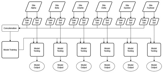
Figure 1.
Dataset fusion procedure. Data from each site are split between train and test sets at a ratio of 80:20.
2.2. Centroid Distance Calculation
Five strategies for data reduction were developed for this paper, four of which use centroid distance as an identifier for reduction. Algorithm 1 shows the process of calculating each centroid distance.
| Algorithm 1 Centroid distance calculation |
|
2.3. Data Reduction Strategies
Once data centroids are calculated, they are used to identify which data to remove from the dataset for training. This paper contains two experiments for data reduction: Data balancing through undersampling and data reduction on both classes, or pure data reduction. Data balancing aims to set the class distribution to 50:50 to alleviate the effects of class imbalance and to reduce the amount of data used by removing data from the dominant class. For example, if a dataset has two classes with 100 and 300 datapoints per class, the data balance methods aim to reduce the majority class from 300 datapoints to 100. In total, this would be a reduction of ((300 − 100)/(100 + 300)) = 50.0%. As this is quite a large reduction, the experimentation described below caps the amounts of reduction by 5%, 10%, 25%, 50%, 75%, as well as the maximum. This allows us to observe the effects of varying the amount of reduction. Pure data reduction aims to identify the effects of reducing data in both classes indiscriminately. For consistency between experiments, the same reduction caps are used as above for pure data reduction. As each site dataset has a different class balance, the maximum amount of data to remove to balance the classes differs across datasets. Datasets with greater class imbalance require more reduction to balance the classes, and vice versa.
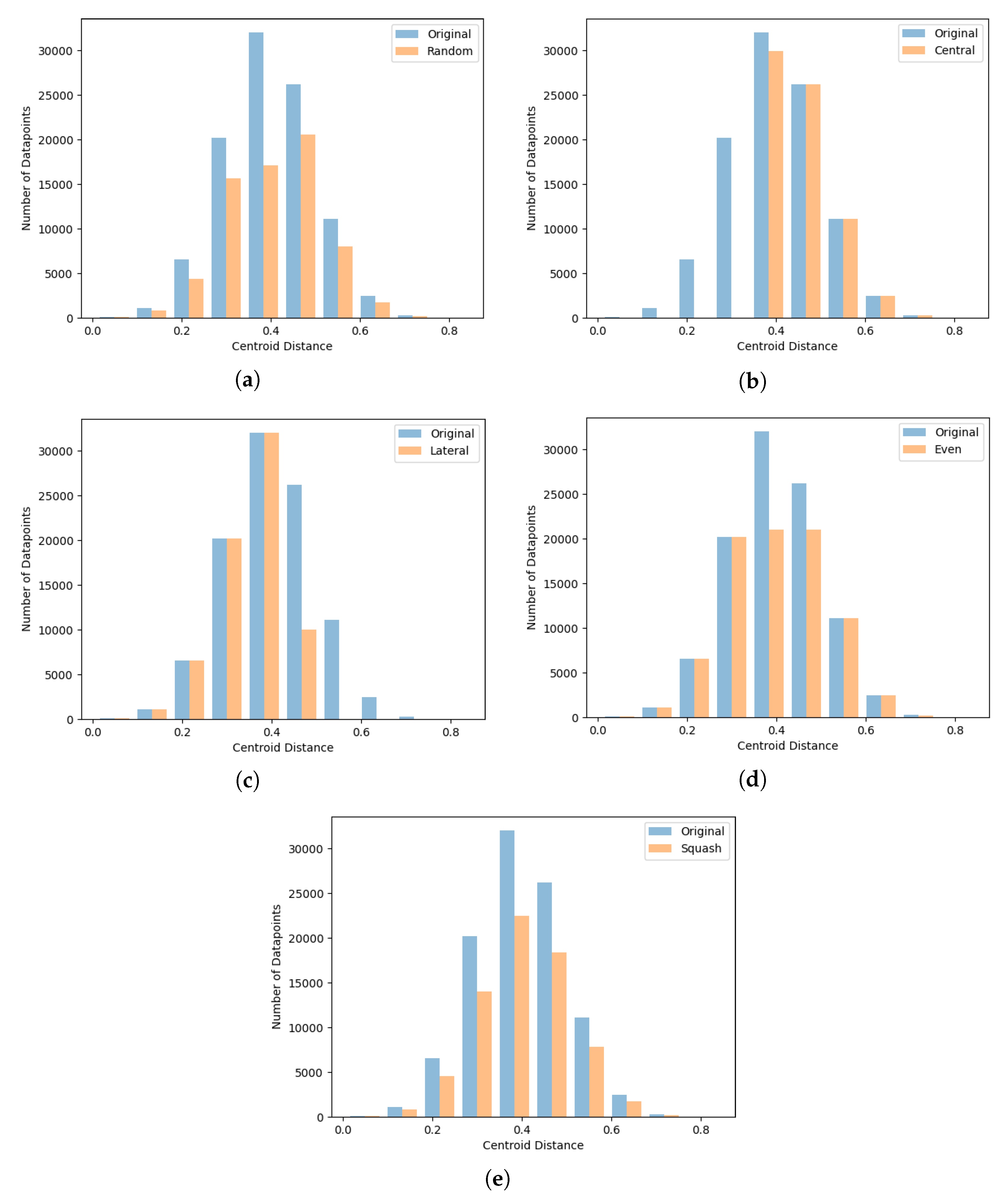
Figure 2 shows the reduction methods developed. These are as follows:
- Random exclusion—random datapoints are removed from the training set.
- Central exclusion—datapoints with the smallest class centroid distance are removed.
- Lateral exclusion—datapoints with the largest class centroid distance are removed.
- Data even—datapoints from the largest density of class centroid distances are removed. This effectively cuts the top off the tallest columns in the centroid distribution plots.
- Data squash—an amount of datapoints proportional to the density of each of 10 bins of data is removed from each bin. This effectively flattens all columns in the centroid distribution plots, proportionally to the size of each column.
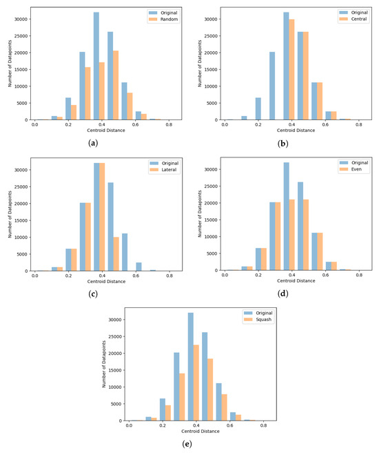
Figure 2.
Centroid distance-based reduction strategies. Original dataset distribution in blue; reduced dataset in orange. (a) Random reduction: Data are removed from the dataset at random. (b) Central reduction: Datapoints with the smallest centroid distance are removed. (c) Lateral reduction: Datapoints with the largest centroid distance are removed. (d) Even reduction: Datapoints from the largest density of centroid distances are removed. (e) Squash reduction: Datapoints are removed proportionally to the local density.
The central and lateral exclusion methods are based on similar work on 2D image data [18], and data even and data squash were developed for this paper.
2.4. Class Density Calculation
Class density, or label density [18,31], is a measure of the aggregate similarity of datapoints within each class of a dataset. A low class density suggests the datapoints of that class are unique, while a high class density suggests many datapoints hold the same features. For the latter case, it stands to reason that similar datapoints may be removed to reduce a dataset without taking away key features from it.
Equation (1) shows how class density is calculated, where d is the density for class i for all n classes, where is the count of samples for that class; is the standard deviations of the m Gaussians of the m-dimensional class i.
For each experiment in this paper, we calculate the class densities to identify the effect the different reduction strategies have on class density. With this knowledge, and the corresponding model performance, we can observe the importance of specific data to overall model performance. We may also use this information to identify if a dataset may be reduced before attempting any data reduction; findings by [18] suggest that by reducing data from the denser classes and converging each class’s density towards a value of 1, model performance may be maintained. We identify if this is true for the HPDMobile dataset and, by extension, other time-series datasets.
2.5. Metrics and Model
Accuracy is traditionally used to measure the performance of AI models, but especially in the case of unbalanced datasets, it is known to give bias to the majority class in a phenomenon known as the accuracy paradox [32]. To avoid this, model performance is also measured by the area under the receiver operating characteristic curve (AUC-ROC) [33]. This is a single value that leverages a model’s sensitivity against its specificity instead of considering these metrics individually, and is considered a more descriptive metric over accuracy for biased datasets for binary classification tasks. The experimental results in this paper show accuracy and AUC-ROC. The p-values of each experiment are also given to show the statistically significant difference between the results and the test benchmark. A p-value below 0.05 is selected to identify statistical significance.
Multiple models were considered for the experimentation, and preliminary testing was performed on each to identify the most suitable model for the rest of the experimentation. Those included were Random Forest (RF), XGBoost, Convolutional Neural Network (CNN), and Long Short-Term Memory (LSTM) models. The RF and XGBoost models are available as part of the scikit-learn library, and the CNN and LSTM models were created using the Pytorch library. Below are the configurations of each network:
- Random Forest Algorithm (RF)
- −
- Maximum depth: unlimited;
- −
- Number of estimators: 100.
- XGBoost
- −
- Maximum depth: unlimited;
- −
- Number of estimators: 100;
- −
- Tree method: ‘approx’.
- Convolutional Neural Network (CNN)
- −
- Layer configuration: 3 convolutional layers with batch normalization; 2 fully connected final layers;
- −
- Learning rate: 0.001;
- −
- Optimiser: Adam;
- −
- Loss function: Binary cross-entropy;
- −
- Data window size: 6 datapoints.
- Long Short-Term Memory Network (LSTM)
- −
- Number of layers: 4 LSTM layers, 1 fully connected layer;
- −
- Hidden layer size: 250;
- −
- Bidirectional: False;
- −
- Learning rate: 0.001;
- −
- Optimiser: Adam;
- −
- Loss function: Binary cross-entropy;
- −
- Data window size: 6 datapoints.
Table 2 shows the results from preliminary testing on Site Alpha of the HPDMobile dataset. This shows that the RF model was the best-performing model. The RF and XGBoost models are the simpler models to train with, while the CNN and LSTM models require the input data’s sequencing to be preserved. This adds a level of complexity which may be avoided by using a model that does not require sequencing preservation. Also, as one objective of this study is for it to be deployable on edge devices with computational constraints, a computationally simpler model would be preferred. The Random Forest model was selected as a simple single-loop model for classification.
Table 2.
Preliminary test results on RF, XGBoost, CNN, and LSTM models with HPDMobile dataset Site Alpha.
2.6. Hardware and Power Calculation
As the focus of this paper is to reduce the cost of operation of occupancy classification on edge devices, it is important to consider the hardware the experiments are carried out on. Due to the large number of experiments and the amount of data logging that will be performed, experimentation is performed on a desktop PC. The code is designed to be transferable to an IOT device for deployment, but in the context of this paper the following hardware is used for experimentation:
- CPU: Intel i7-11700k;
- RAM: 16 GB DDR4;
- OS: Windows 10.
The power consumption of the CPU is measured using HWiNFO software [34] while the model is trained. For the processor used, the power consumption is 14 W when idle and 46 W when busy. The power consumption of the program is the difference between these two: 32 W. This value is consistent between experiments regardless of tree depth or dataset size, although these factors instead increase the runtime of training. In the UK, according to the Department for Energy Security and Net Zero [35], this translates to 6.623 g of CO2 emissions per hour.
3. Results
3.1. Experiments on Individual Sites
For each experiment performed, the datasets were split into training and testing sets at a ratio of 80:20. Each experiment was run five times and results were averaged.
Experimentation was performed to observe the effects of reducing the data by varying amounts, from different areas in the data distribution. Due to the different class balances of each dataset, class balancing removes more data for more imbalanced classes, and vice versa. Table 3 shows the maximum percentage reduction of the larger class, and the dataset overall. It also shows the densities of the classes, derived from research in [18]. This will be used as a metric to identify suitability for data reduction.
Table 3.
HPDMobile class balance and class density properties, and maximum reduction amounts after class balancing.
3.1.1. Experimental Benchmark
Before data reduction was performed, the models were trained with the full dataset to acquire the benchmark results. These results are shown in Table 4. The runtime of each of these experiments was less than one minute.
Table 4.
Experimental benchmarks of accuracy and AUC-ROC with RF model.
3.1.2. Site Alpha
Site Alpha has 147,750 datapoints and a class balance of 20:80. Figure 3 shows the results of varying degrees of data reduction on the single dataset. Table 5 and Table 6 show the p-values of the AUC-ROC of each experiment.
Figure 3a,b show that model accuracy decreases steadily as more data are removed, regardless of whether the removed data are from the majority class or both. Figure 3c,d, show a similar drop in performance. The AUC-ROC score may be maintained with majority class reduction, up to 50%. This is interesting behaviour as the accuracy up to this amount of reduction decreases. By performing reduction in this way, we may improve the model’s ability to avoid false positives and false negatives. It is also important to note that the p-values of all experiments corresponding to majority class reduction indicate that the results are not statistically differentiable from the benchmark, apart from with the maximum reduction. For the maximum reduction, the performance is clearly worse, hence the differentiation. For every other case, performance is maintained while reducing the amount of data.
Table 7 and Table 8 show the class densities for each experiment. Table 7 shows that, for each reduction method, the densities of each class become closer, up to a reduction cap of 50%. At maximum reduction, the minority class, class 0, has a greater class density than class 1. At the same time, both the accuracy and the AUC-ROC of the model decrease by a relatively large amount. This supports the theory that data may be reduced in order to balance the density of each class towards a value of 1, but further reduction that leads to an imbalance causes the model to deteriorate. Also, Table 8 shows that by performing data reduction on both classes, the difference in class density between classes 0 and 1 does not change by a significant amount. This may explain why the accuracy and AUR-ROC decrease as the amount of data is reduced, while they do not with reduction only on the majority class.
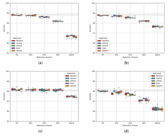
Figure 3.
Experimental results for Site Alpha test set. (a) Accuracy, Majority class reduced; (b) Accuracy, Both classes reduced; (c) AUC, Majority class reduced; (d) AUC, Both classes reduced.
Figure 3.
Experimental results for Site Alpha test set. (a) Accuracy, Majority class reduced; (b) Accuracy, Both classes reduced; (c) AUC, Majority class reduced; (d) AUC, Both classes reduced.
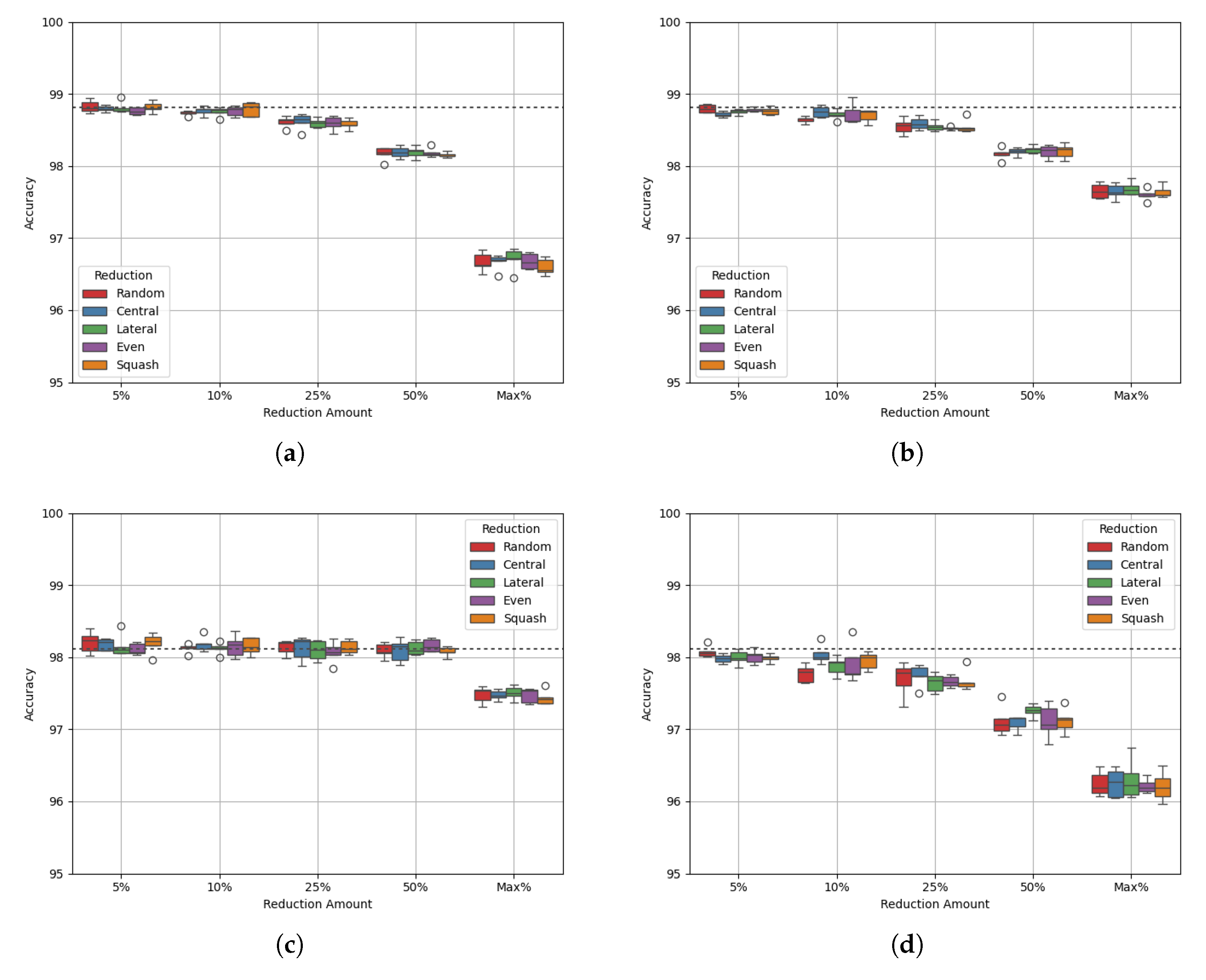
Table 5.
p-values of the AUC metrics of each experiment of reduction on the majority class, on Site Alpha test set. Values marked with an * have a statistically significant difference from the benchmark.
Table 5.
p-values of the AUC metrics of each experiment of reduction on the majority class, on Site Alpha test set. Values marked with an * have a statistically significant difference from the benchmark.
| Reduction | Random | Central | Lateral | Even | Squash |
|---|---|---|---|---|---|
| 5% | 0.268 | 0.182 | 0.616 | 0.794 | 0.329 |
| 10% | 0.971 | 0.255 | 0.906 | 0.652 | 0.625 |
| 25% | 0.74 | 0.972 | 0.688 | 0.482 | 0.673 |
| 50% | 0.605 | 0.731 | 0.948 | 0.341 | 0.239 |
| Max | 2.25 * | 2.63 * | 1.49 * | 1.59 * | 1.18 * |
Table 6.
p-values of the AUC metrics of each experiment of reduction on both classes, on Site Alpha test set. Values marked with an * have a statistically significant difference from the benchmark.
Table 6.
p-values of the AUC metrics of each experiment of reduction on both classes, on Site Alpha test set. Values marked with an * have a statistically significant difference from the benchmark.
| Reduction | Random | Central | Lateral | Even | Squash |
|---|---|---|---|---|---|
| 5% | 0.273 | 7.04 * | 4.42 * | 5.92 | 5.56 * |
| 10% | 3.51 * | 0.267 | 1.44 * | 0.16 | 3.48 * |
| 25% | 1.71 * | 5.21 * | 1.21 * | 1.98 * | 2.83 * |
| 50% | 3.96 * | 2.56 * | 2.64 * | 7.09 * | 2.11 * |
| Max | 1.85 * | 3.14 * | 1.25 * | 1.73 * | 3.52 * |
Table 7.
Class density of Site Alpha dataset after data reduction on the majority class only. R: random reduction, C: central reduction, L: lateral reduction, E: even reduction, S: squash reduction.
Table 7.
Class density of Site Alpha dataset after data reduction on the majority class only. R: random reduction, C: central reduction, L: lateral reduction, E: even reduction, S: squash reduction.
| Class 0 (Not Occupied) | Class 1 (Occupied) | |||||||||
|---|---|---|---|---|---|---|---|---|---|---|
|
Data Reduced | R | C | L | E | S | R | C | L | E | S |
| 5% | 0.707 | 0.712 | 0.670 | 0.687 | 0.704 | 1.565 | 1.565 | 1.582 | 1.565 | 1.551 |
| 10% | 0.739 | 0.721 | 0.722 | 0.756 | 0.740 | 1.565 | 1.562 | 1.552 | 1.511 | 1.550 |
| 25% | 0.812 | 0.875 | 0.848 | 0.848 | 0.882 | 1.507 | 1.485 | 1.482 | 1.389 | 1.447 |
| 50% | 1.112 | 1.185 | 1.176 | 1.161 | 1.133 | 1.324 | 1.308 | 1.315 | 1.112 | 1.311 |
| Max | 1.782 | 1.734 | 1.725 | 1.796 | 1.621 | 1.008 | 1.010 | 0.977 | 0.680 | 0.968 |
Table 8.
Class density of Site Alpha dataset after data reduction across both classes. R: random reduction, C: central reduction, L: lateral reduction, E: even reduction, S: squash reduction.
Table 8.
Class density of Site Alpha dataset after data reduction across both classes. R: random reduction, C: central reduction, L: lateral reduction, E: even reduction, S: squash reduction.
| Class 0 (Not Occupied) | Class 1 (Occupied) | |||||||||
|---|---|---|---|---|---|---|---|---|---|---|
|
Data Reduced | R | C | L | E | S | R | C | L | E | S |
| 5% | 0.720 | 0.706 | 0.719 | 0.643 | 0.707 | 1.549 | 1.555 | 1.579 | 1.591 | 1.572 |
| 10% | 0.782 | 0.669 | 0.634 | 0.704 | 0.709 | 1.565 | 1.579 | 1.598 | 1.532 | 1.557 |
| 25% | 0.792 | 0.752 | 0.781 | 0.635 | 0.622 | 1.562 | 1.573 | 1.580 | 1.531 | 1.597 |
| 50% | 0.707 | 0.716 | 0.735 | 0.595 | 0.633 | 1.571 | 1.569 | 1.582 | 1.458 | 1.579 |
| Max | 0.766 | 0.804 | 0.850 | 0.554 | 0.541 | 1.556 | 1.571 | 1.622 | 1.340 | 1.594 |
3.1.3. Site Beta
Site Beta has 146,879 datapoints and a class balance of 40:60. This dataset has relatively few datapoints and less class imbalance than the others in the HPDMobile dataset, causing a lower maximum reduction of 34%. Figure 4 shows the results of varying degrees of data reduction on the Site Beta dataset, and Table 9 and Table 10 show the p-values of the AUC-ROC of each experiment.
Both the accuracy and AUC-ROC values change by less that 0.2% as the amount of data is reduced. This is due to much less reduction being required to balance the classes, compared to the reduction performed for Site Alpha. However, there is still a very slight drop in both accuracy and AUC-ROC. Most of the p-values show no statistically significant difference from the benchmark, expect for some of the more extreme reduction amounts. These results show a larger difference from the benchmark, which raises questions about the stability of the model after reducing the dataset.
Table 11 and Table 12 show that the densities of both classes are values above 1 for all experiments except the maximum reduction of the majority class, where class 1’s density is between 0.9 and 1. This suggests that the reduction methods performed are not enough to shift the densities towards 1. Alternative methods may be required to optimise datasets like Site Beta, where classes are already closely balanced.
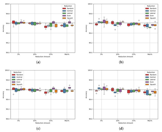
Figure 4.
Experimental results for Site Beta test set. (a) Accuracy, Majority class reduced; (b) Accuracy, Both classes reduced; (c) AUC, Majority class reduced; (d) AUC, Both classes reduced.
Figure 4.
Experimental results for Site Beta test set. (a) Accuracy, Majority class reduced; (b) Accuracy, Both classes reduced; (c) AUC, Majority class reduced; (d) AUC, Both classes reduced.
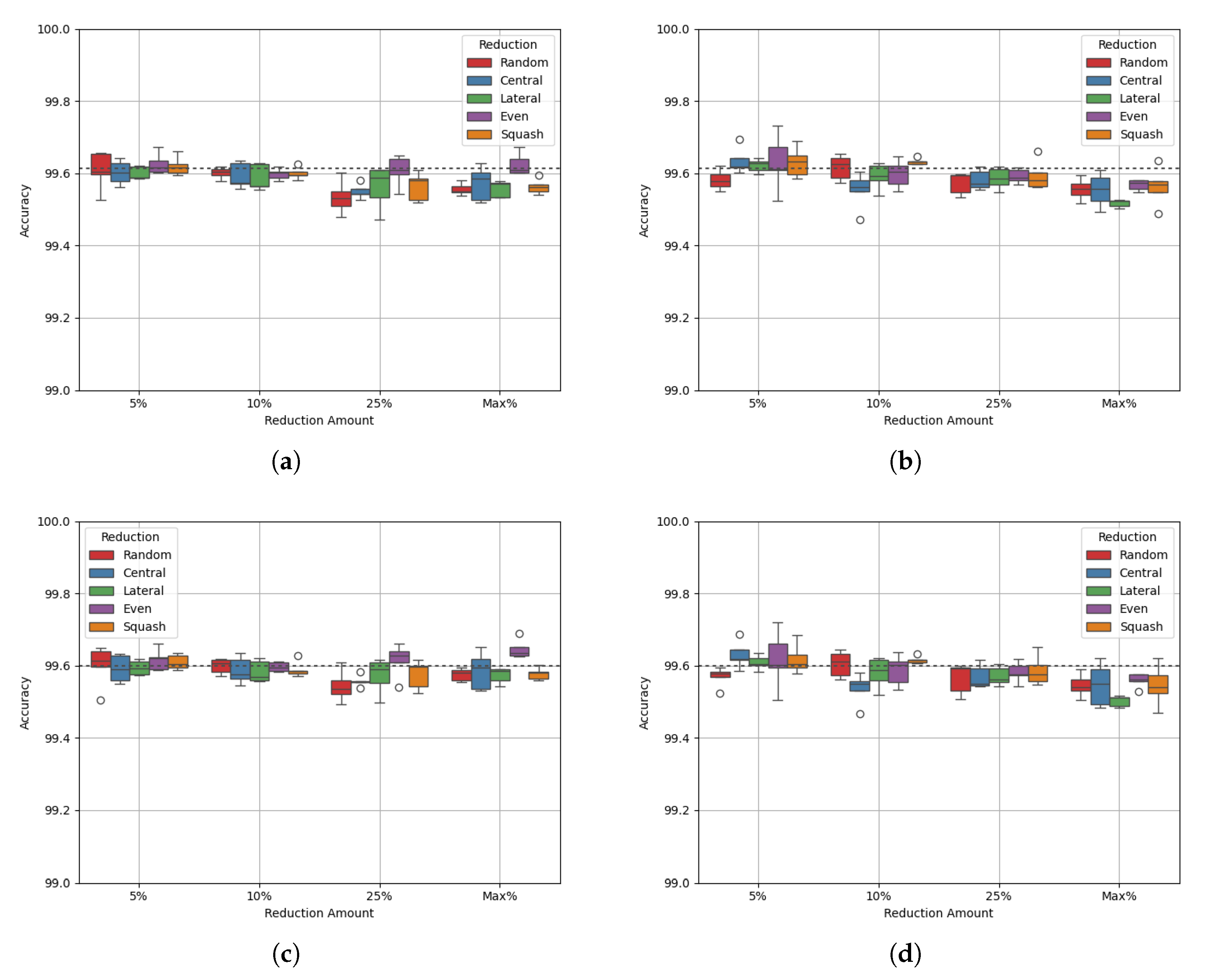
Table 9.
p-values of the AUC metrics of each experiment of reduction on the majority class, on Site Beta test set. Values marked with an * have a statistically significant difference from the benchmark.
Table 9.
p-values of the AUC metrics of each experiment of reduction on the majority class, on Site Beta test set. Values marked with an * have a statistically significant difference from the benchmark.
| Reduction | Random | Central | Lateral | Even | Squash |
|---|---|---|---|---|---|
| 5% | 0.955 | 0.684 | 0.591 | 0.258 | 0.325 |
| 10% | 0.929 | 0.486 | 0.32 | 0.672 | 0.376 |
| 25% | 4.65 * | 4.82 * | 0.297 | 0.483 | 0.251 |
| Max | 3.47 * | 0.589 | 5.31 | 1.71 * | 4.05 * |
Table 10.
p-values of the AUC metrics of each experiment of reduction on both classes, on Site Beta test set. Values marked with an * have a statistically significant difference from the benchmark.
Table 10.
p-values of the AUC metrics of each experiment of reduction on both classes, on Site Beta test set. Values marked with an * have a statistically significant difference from the benchmark.
| Reduction | Random | Central | Lateral | Even | Squash |
|---|---|---|---|---|---|
| 5% | 7.27 | 0.151 | 0.349 | 0.657 | 0.368 |
| 10% | 0.784 | 3.04 * | 0.389 | 0.564 | 2.12 * |
| 25% | 0.142 | 0.111 | 7.13 | 0.247 | 0.523 |
| Max | 1.80 * | 0.124 | 1.38 * | 1.00 * | 9.75 |
Table 11.
Class density of Site Beta dataset after data reduction on the majority class only. R: random reduction, C: central reduction, L: lateral reduction, E: even reduction, S: squash reduction.
Table 11.
Class density of Site Beta dataset after data reduction on the majority class only. R: random reduction, C: central reduction, L: lateral reduction, E: even reduction, S: squash reduction.
| Class 0 (Not Occupied) | Class 1 (Occupied) | |||||||||
|---|---|---|---|---|---|---|---|---|---|---|
|
Data Reduced | R | C | L | E | S | R | C | L | E | S |
| 5% | 1.111 | 1.132 | 1.112 | 1.114 | 1.126 | 1.172 | 1.153 | 1.164 | 1.157 | 1.149 |
| 10% | 1.144 | 1.157 | 1.162 | 1.149 | 1.158 | 1.137 | 1.146 | 1.146 | 1.119 | 1.120 |
| 25% | 1.277 | 1.276 | 1.279 | 1.263 | 1.298 | 1.055 | 1.047 | 1.035 | 1.004 | 1.021 |
| Max | 1.383 | 1.345 | 1.371 | 1.345 | 1.387 | 0.963 | 1.002 | 0.970 | 0.917 | 0.952 |
Table 12.
Class density of Site Beta dataset after each data reduction method, with reduction on both classes. R: random reduction, C: central reduction, L: lateral reduction, E: even reduction, S: squash reduction.
Table 12.
Class density of Site Beta dataset after each data reduction method, with reduction on both classes. R: random reduction, C: central reduction, L: lateral reduction, E: even reduction, S: squash reduction.
| Class 0 (Not Occupied) | Class 1 (Occupied) | |||||||||
|---|---|---|---|---|---|---|---|---|---|---|
|
Data Reduced | R | C | L | E | S | R | C | L | E | S |
| 5% | 1.083 | 1.097 | 1.087 | 1.091 | 1.071 | 1.195 | 1.180 | 1.198 | 1.180 | 1.189 |
| 10% | 1.087 | 1.088 | 1.094 | 1.062 | 1.079 | 1.191 | 1.194 | 1.192 | 1.187 | 1.177 |
| 25% | 1.057 | 1.078 | 1.085 | 1.047 | 1.061 | 1.205 | 1.198 | 1.186 | 1.156 | 1.185 |
| Max | 1.085 | 1.138 | 1.114 | 1.052 | 1.068 | 1.190 | 1.184 | 1.218 | 1.126 | 1.174 |
3.1.4. Site Charlie
Site Charlie has one of the larger class imbalances, and therefore larger maximum reduction caps, with a maximum reduction of 72%. It is also one of the larger datasets, with over 300,000 datapoints. Figure 5 shows the experimental results and Table 13 and Table 14 show the p-values of the AUC-ROC of each experiment.
Figure 5a shows that up to a reduction cap of 50%, accuracy is above the benchmark, with the lateral data reduction method with a reduction cap of 10% performing best. With the maximum reduction cap (at 72.111%), however, the performance is below the benchmark for all strategies. This indicates a delicate balance is needed for data reduction to ensure that too much data is not removed. This is further explained by the class densities; Table 15 shows that as more of the majority class is reduced, both classes’ densities converge around a value of 1. At a reduction cap of 50%, the combined difference between each density and 1 is smallest, which is where the AUC-ROC is greatest across all strategies. However, the results are less stable, as shown by the size of each box. Furthermore, Table 16 shows that by reducing data across both classes, the model performance is worse.
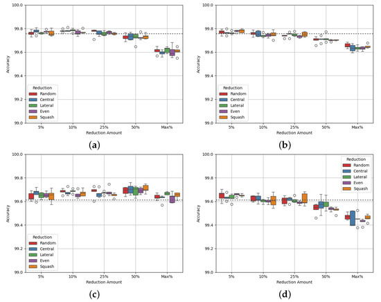
Figure 5.
Experimental results for Site Charlie test set. (a) Accuracy, Majority class reduced; (b) Accuracy, Both classes reduced; (c) AUC, Majority class reduced; (d) AUC, Both classes reduced.
Figure 5.
Experimental results for Site Charlie test set. (a) Accuracy, Majority class reduced; (b) Accuracy, Both classes reduced; (c) AUC, Majority class reduced; (d) AUC, Both classes reduced.
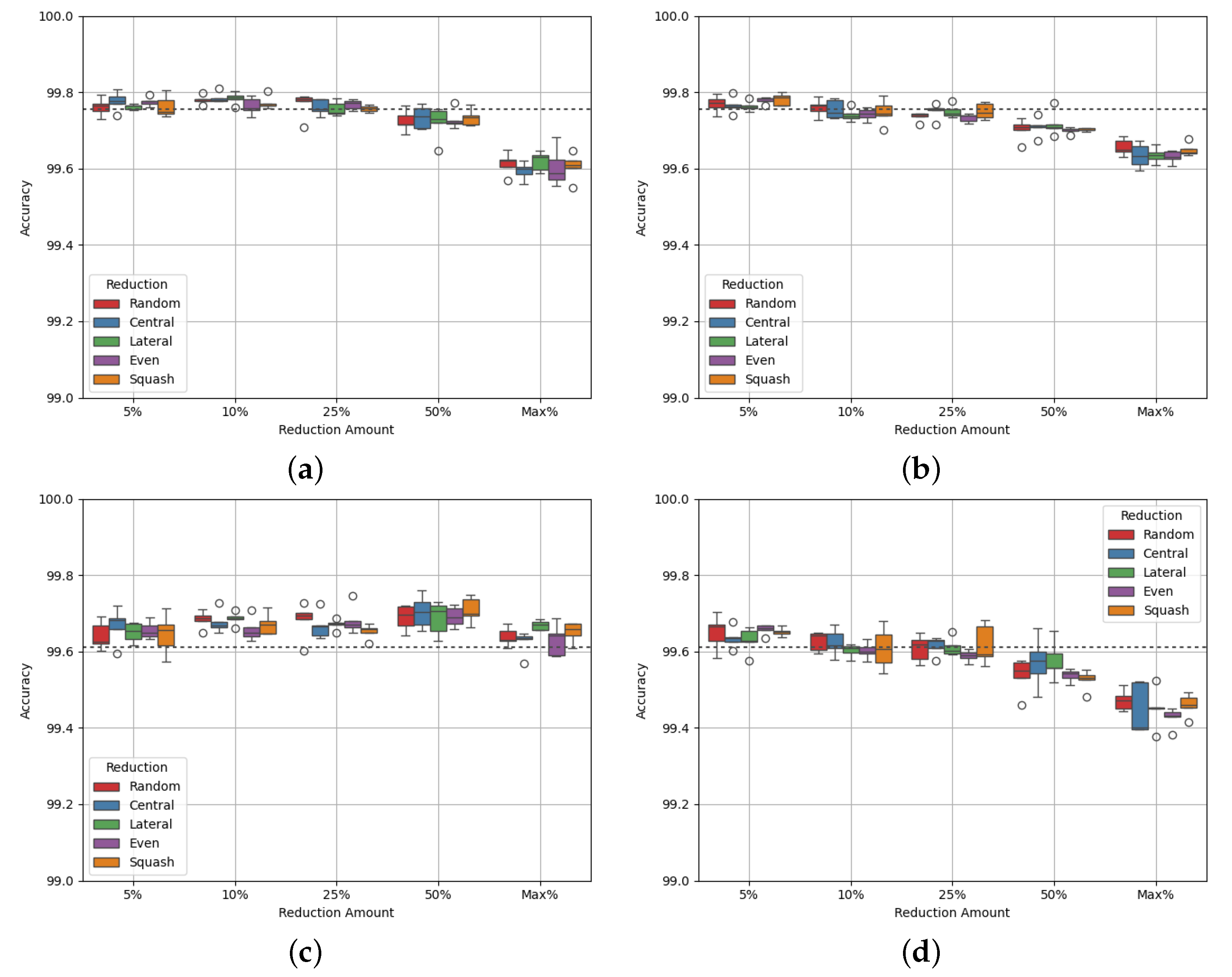
Table 13.
p-values of the AUC metrics of each experiment of reduction on the majority class, on Site Charlie test set. Values marked with an * have a statistically significant difference from the benchmark.
Table 13.
p-values of the AUC metrics of each experiment of reduction on the majority class, on Site Charlie test set. Values marked with an * have a statistically significant difference from the benchmark.
| Reduction | Random | Central | Lateral | Even | Squash |
|---|---|---|---|---|---|
| 5% | 0.14 | 4.96 * | 3.08 * | 1.18 * | 0.215 |
| 10% | 2.05 * | 7.93 * | 6.49 * | 2.93 * | 8.29 * |
| 25% | 2.96 * | 2.23 * | 6.12 * | 1.41 * | 8.71 * |
| 50% | 6.60 * | 9.01 * | 1.74 * | 2.63 * | 3.41 * |
| Max | 7.02 | 0.389 | 4.31 * | 0.365 | 2.89 * |
Table 14.
p-values of the AUC metrics of each experiment of reduction on both classes, on Site Charlie test set. Values marked with an * have a statistically significant difference from the benchmark.
Table 14.
p-values of the AUC metrics of each experiment of reduction on both classes, on Site Charlie test set. Values marked with an * have a statistically significant difference from the benchmark.
| Reduction | Random | Central | Lateral | Even | Squash |
|---|---|---|---|---|---|
| 5% | 0.138 | 0.116 | 0.299 | 1.71 * | 1.23 * |
| 10% | 0.233 | 0.461 | 0.3 | 0.396 | 0.924 |
| 25% | 0.863 | 0.705 | 0.994 | 2.66 * | 0.804 |
| 50% | 2.42 * | 0.255 | 0.194 | 6.01 * | 2.02 * |
| Max | 3.48 * | 5.56 * | 2.32 * | 9.48 * | 3.73 * |
Table 15.
Class density of Site Charlie dataset after data reduction on the majority class only. R: random reduction, C: central reduction, L: lateral reduction, E: even reduction, S: squash reduction.
Table 15.
Class density of Site Charlie dataset after data reduction on the majority class only. R: random reduction, C: central reduction, L: lateral reduction, E: even reduction, S: squash reduction.
| Class 0 (Not Occupied) | Class 1 (Occupied) | |||||||||
|---|---|---|---|---|---|---|---|---|---|---|
| Data Reduced | R | C | L | E | S | R | C | L | E | S |
| 5% | 0.663 | 0.662 | 0.664 | 0.663 | 0.661 | 1.512 | 1.524 | 1.519 | 1.511 | 1.513 |
| 10% | 0.689 | 0.689 | 0.690 | 0.693 | 0.695 | 1.492 | 1.493 | 1.491 | 1.487 | 1.489 |
| 25% | 0.794 | 0.793 | 0.793 | 0.791 | 0.791 | 1.449 | 1.423 | 1.421 | 1.403 | 1.414 |
| 50% | 1.046 | 1.033 | 1.046 | 1.048 | 1.042 | 1.260 | 1.271 | 1.222 | 1.202 | 1.251 |
| Max | 1.458 | 1.466 | 1.460 | 1.457 | 1.467 | 0.985 | 0.981 | 0.991 | 0.891 | 0.957 |
Table 16.
Class density of Site Charlie dataset after data reduction across both classes. R: random reduction, C: central reduction, L: lateral reduction, E: even reduction, S: squash reduction.
Table 16.
Class density of Site Charlie dataset after data reduction across both classes. R: random reduction, C: central reduction, L: lateral reduction, E: even reduction, S: squash reduction.
| Class 0 (Not Occupied) | Class 1 (Occupied) | |||||||||
|---|---|---|---|---|---|---|---|---|---|---|
| Data Reduced | R | C | L | E | S | R | C | L | E | S |
| 5% | 0.636 | 0.637 | 0.640 | 0.637 | 0.636 | 1.531 | 1.541 | 1.531 | 1.529 | 1.530 |
| 10% | 0.638 | 0.639 | 0.639 | 0.632 | 0.637 | 1.534 | 1.532 | 1.531 | 1.525 | 1.528 |
| 25% | 0.635 | 0.635 | 0.638 | 0.636 | 0.635 | 1.538 | 1.537 | 1.526 | 1.512 | 1.522 |
| 50% | 0.639 | 0.636 | 0.635 | 0.633 | 0.633 | 1.533 | 1.538 | 1.526 | 1.489 | 1.512 |
| Max | 0.634 | 0.646 | 0.638 | 0.631 | 0.631 | 1.556 | 1.563 | 1.554 | 1.445 | 1.509 |
3.1.5. Site Delta
Site Delta has similar properties to Site Alpha, with 146,879 datapoints and a class balance of 21:79. Figure 6 shows the experimental results, and Table 17 and Table 18 show the p-values of the AUC-ROC of each experiment.
Figure 6a,b show similar behaviour to each other, where accuracy drops as greater reduction is performed. Figure 6c shows that the AUC-ROC is maintained up to a 75% reduction for class balance. However, Figure 6d shows that the AUC-ROC drops by a larger amount with reduction across both classes. Site Delta has a large class imbalance, which suggests that some balancing is important for optimal results. The p-values of the results for all but three experiments (data squash at 10% and maximum reduction and lateral reduction at 25% reduction) show no statistically significant difference from the benchmark. This suggests once again that through this method of data reduction, optimal model performance is maintained.
Table 19 and Table 20 show the class densities after each reduction method for Site Delta. As with the other sites, reduction on both classes does little to bring the class densities towards a value of 1. For majority class reduction, an optimal amount of reduction to achieve balanced class densities is between reduction caps of 50% and 75%. This demonstrates the delicate balance needed to find the optimal amount of data to remove for the best performance.
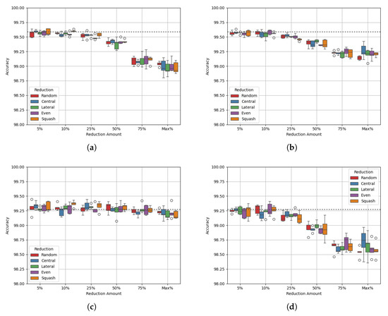
Figure 6.
Experimental results for Site Delta test set. (a) Accuracy, Majority class reduced; (b) Accuracy, Both classes reduced; (c) AUC, Majority class reduced; (d) AUC, Both classes reduced.
Figure 6.
Experimental results for Site Delta test set. (a) Accuracy, Majority class reduced; (b) Accuracy, Both classes reduced; (c) AUC, Majority class reduced; (d) AUC, Both classes reduced.
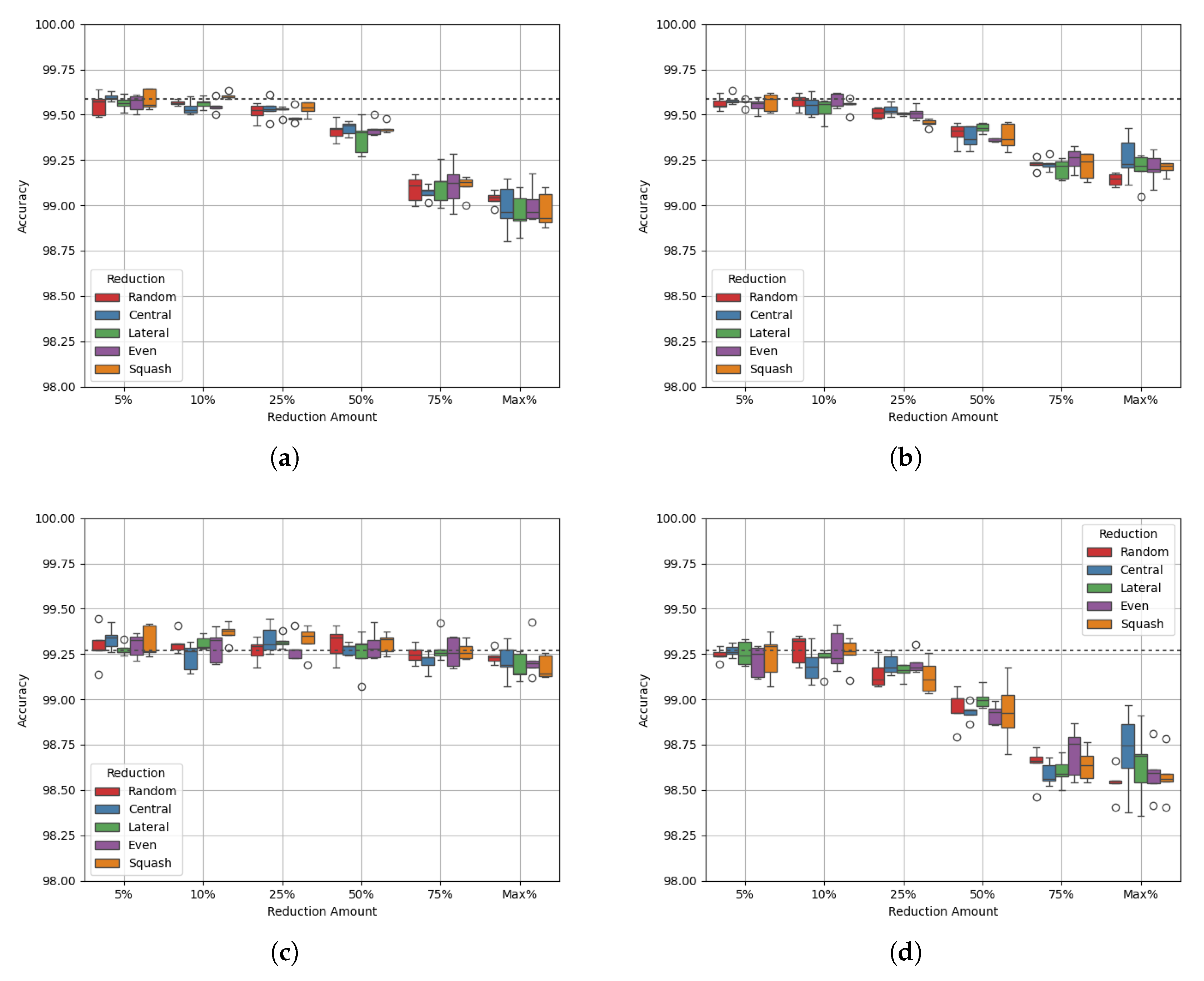
Table 17.
p-values of the AUC metrics of each experiment of reduction on the majority class, on Site Delta test set. Values marked with an * have a statistically significant difference from the benchmark.
Table 17.
p-values of the AUC metrics of each experiment of reduction on the majority class, on Site Delta test set. Values marked with an * have a statistically significant difference from the benchmark.
| Reduction | Random | Central | Lateral | Even | Squash |
|---|---|---|---|---|---|
| 5% | 0.704 | 8.17 | 0.711 | 0.396 | 0.287 |
| 10% | 0.199 | 0.35 | 7.70 | 0.582 | 1.59 * |
| 25% | 0.949 | 0.168 | 4.32 * | 0.757 | 0.212 |
| 50% | 0.415 | 0.553 | 0.807 | 0.473 | 0.184 |
| 75% | 0.375 | 5.83 | 0.778 | 0.802 | 0.891 |
| Max | 0.113 | 0.254 | 5.27 | 0.444 | 3.14 * |
Table 18.
p-values of the AUC metrics of each experiment of reduction on both classes, on Site Delta test set. Values marked with an * have a statistically significant difference from the benchmark.
Table 18.
p-values of the AUC metrics of each experiment of reduction on both classes, on Site Delta test set. Values marked with an * have a statistically significant difference from the benchmark.
| Reduction | Random | Central | Lateral | Even | Squash |
|---|---|---|---|---|---|
| 5% | 0.198 | 0.918 | 0.625 | 0.226 | 0.591 |
| 10% | 0.869 | 0.144 | 0.155 | 0.967 | 0.686 |
| 25% | 2.07 * | 3.73 * | 3.20 * | 5.53 | 2.61 * |
| 50% | 2.98 * | 1.00 * | 4.39 * | 1.59 * | 1.42 * |
| 75% | 1.70 * | 2.11 * | 4.50 * | 8.12 * | 1.02 * |
| Max | 5.72 * | 5.59 * | 2.34 * | 4.75 * | 3.29 * |
Table 19.
Class density of Site Delta dataset after data reduction on the majority class only. R: random reduction, C: central reduction, L: lateral reduction, E: even reduction, S: squash reduction.
Table 19.
Class density of Site Delta dataset after data reduction on the majority class only. R: random reduction, C: central reduction, L: lateral reduction, E: even reduction, S: squash reduction.
| Class 0 (Not Occupied) | Class 1 (Occupied) | |||||||||
|---|---|---|---|---|---|---|---|---|---|---|
| Data Reduced | R | C | L | E | S | R | C | L | E | S |
| 5% | 0.578 | 0.561 | 0.586 | 0.556 | 0.559 | 1.566 | 1.573 | 1.553 | 1.549 | 1.550 |
| 10% | 0.633 | 0.586 | 0.603 | 0.633 | 0.590 | 1.534 | 1.559 | 1.544 | 1.504 | 1.523 |
| 25% | 0.671 | 0.679 | 0.662 | 0.675 | 0.645 | 1.475 | 1.520 | 1.503 | 1.414 | 1.468 |
| 50% | 0.932 | 0.969 | 0.938 | 0.954 | 0.914 | 1.334 | 1.412 | 1.352 | 1.152 | 1.294 |
| 75% | 1.354 | 1.494 | 1.484 | 1.493 | 1.420 | 1.052 | 1.052 | 1.103 | 0.737 | 0.957 |
| Max | 1.506 | 1.456 | 1.583 | 1.531 | 1.509 | 1.074 | 1.062 | 0.969 | 0.685 | 0.909 |
Table 20.
Class density of Site Delta dataset after data reduction across both classes. R: random reduction, C: central reduction, L: lateral reduction, E: even reduction, S: squash reduction.
Table 20.
Class density of Site Delta dataset after data reduction across both classes. R: random reduction, C: central reduction, L: lateral reduction, E: even reduction, S: squash reduction.
| Class 0 (Not Occupied) | Class 1 (Occupied) | |||||||||
|---|---|---|---|---|---|---|---|---|---|---|
| Data Reduced | R | C | L | E | S | R | C | L | E | S |
| 5% | 0.533 | 0.544 | 0.558 | 0.577 | 0.578 | 1.577 | 1.572 | 1.573 | 1.553 | 1.555 |
| 10% | 0.563 | 0.516 | 0.561 | 0.542 | 0.557 | 1.605 | 1.600 | 1.579 | 1.549 | 1.557 |
| 25% | 0.627 | 0.545 | 0.546 | 0.518 | 0.567 | 1.581 | 1.577 | 1.572 | 1.512 | 1.540 |
| 50% | 0.602 | 0.634 | 0.559 | 0.515 | 0.537 | 1.663 | 1.591 | 1.573 | 1.416 | 1.538 |
| 75% | 0.615 | 0.569 | 0.581 | 0.464 | 0.632 | 1.639 | 1.704 | 1.634 | 1.299 | 1.498 |
| Max | 0.573 | 0.562 | 0.663 | 0.445 | 0.629 | 1.688 | 1.593 | 1.615 | 1.278 | 1.474 |
3.1.6. Site Epsilon
Site Epsilon is the smallest site in the dataset, with only 129,599 datapoints. It is also among the most imbalanced of the site datasets, with a class balance of 24:76. Figure 7 shows the experimental results, and Table 21 and Table 22 show the p-values of the AUC-ROC of each experiment.
Much like with Site Delta, Figure 7a,b show that data reduction causes a drop in performance of up to 0.4%. Like the experiments for sites Alpha, Beta, and Delta, the AUC-ROC does not decrease with accuracy until the maximum reduction.
Table 23 shows that with each reduction cap, the density of class 0 increases while the density of class 1 decreases, as with the other sites. However, class 0’s density passes through a value of 1 between reduction caps of 10% and 25%, while class 1 passes through a value of 1 between a reduction cap of 50% and the maximum (for allreduction methods except random). This makes it difficult to identify the best reduction cap for this dataset. Perhaps an alternative method of data reduction would be more appropriate. Table 24 shows that, similarly to sites Charlie and Delta, as data is reduced the densities move further from a value of 1. This is linked to a drop in both accuracy and AUC-ROC.
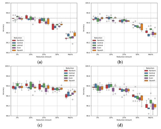
Figure 7.
Experimental results for Site Epsilon test set. (a) Accuracy, Majority class reduced; (b) Accuracy, Both classes reduced; (c) AUC, Majority class reduced; (d) AUC, Both classes reduced.
Figure 7.
Experimental results for Site Epsilon test set. (a) Accuracy, Majority class reduced; (b) Accuracy, Both classes reduced; (c) AUC, Majority class reduced; (d) AUC, Both classes reduced.
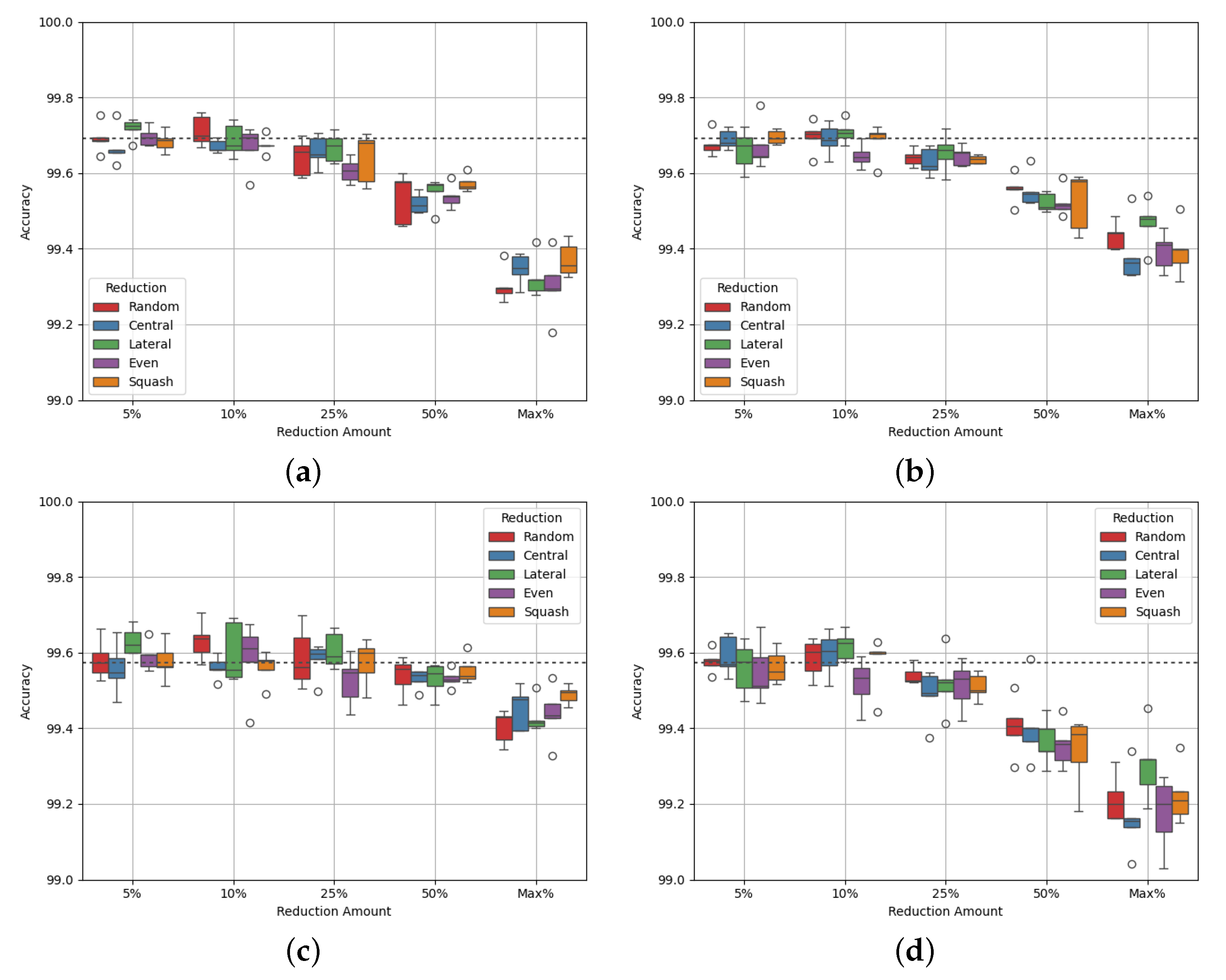
Table 21.
p-values of the AUC metrics of each experiment of reduction on the majority class, on Site Epsilon test set. Values marked with an * have a statistically significant difference from the benchmark.
Table 21.
p-values of the AUC metrics of each experiment of reduction on the majority class, on Site Epsilon test set. Values marked with an * have a statistically significant difference from the benchmark.
| Reduction | Random | Central | Lateral | Even | Squash |
|---|---|---|---|---|---|
| 5% | 0.761 | 0.618 | 2.51 * | 0.376 | 0.919 |
| 10% | 6.61 | 0.373 | 0.541 | 0.844 | 0.522 |
| 25% | 0.745 | 0.765 | 0.207 | 0.173 | 0.991 |
| 50% | 0.186 | 1.91 * | 8.94 | 1.57 * | 0.282 |
| Max | 1.03 * | 8.73 * | 1.79 * | 1.47 * | 1.37 * |
Table 22.
p-values of the AUC metrics of each experiment of reduction on both classes, on Site Epsilon test set. Values marked with an * have a statistically significant difference from the benchmark.
Table 22.
p-values of the AUC metrics of each experiment of reduction on both classes, on Site Epsilon test set. Values marked with an * have a statistically significant difference from the benchmark.
| Reduction | Random | Central | Lateral | Even | Squash |
|---|---|---|---|---|---|
| 5% | 0.856 | 0.513 | 0.676 | 0.513 | 0.593 |
| 10% | 0.639 | 0.447 | 6.03 | 0.127 | 0.997 |
| 25% | 3.89 * | 4.75 * | 0.203 | 0.105 | 1.51 * |
| 50% | 7.18 * | 2.48 * | 1.58 * | 1.21 * | 5.37 * |
| Max | 2.01 * | 1.07 * | 3.55 * | 8.09 * | 5.19 * |
Table 23.
Class density of Site Epsilon dataset after data reduction on the majority class only. R: random reduction, C: central reduction, L: lateral reduction, E: even reduction, S: squash reduction.
Table 23.
Class density of Site Epsilon dataset after data reduction on the majority class only. R: random reduction, C: central reduction, L: lateral reduction, E: even reduction, S: squash reduction.
| Class 0 (Not Occupied) | Class 1 (Occupied) | |||||||||
|---|---|---|---|---|---|---|---|---|---|---|
| Data Reduced | R | C | L | E | S | R | C | L | E | S |
| 5% | 0.862 | 0.932 | 0.878 | 0.909 | 0.907 | 1.383 | 1.378 | 1.391 | 1.363 | 1.370 |
| 10% | 0.944 | 0.946 | 0.956 | 0.969 | 0.954 | 1.377 | 1.341 | 1.369 | 1.325 | 1.340 |
| 25% | 1.061 | 1.041 | 1.079 | 1.115 | 1.050 | 1.319 | 1.302 | 1.279 | 1.207 | 1.265 |
| 50% | 1.406 | 1.400 | 1.458 | 1.406 | 1.456 | 1.200 | 1.124 | 1.168 | 0.963 | 1.097 |
| Max | 1.834 | 1.790 | 1.813 | 1.836 | 1.814 | 1.008 | 0.977 | 0.973 | 0.692 | 0.935 |
Table 24.
Class density of Site Epsilon dataset after data reduction across both classes. R: random reduction, C: central reduction, L: lateral reduction, E: even reduction, S: squash reduction.
Table 24.
Class density of Site Epsilon dataset after data reduction across both classes. R: random reduction, C: central reduction, L: lateral reduction, E: even reduction, S: squash reduction.
| Class 0 (Not Occupied) | Class 1 (Occupied) | |||||||||
|---|---|---|---|---|---|---|---|---|---|---|
| Data Reduced | R | C | L | E | S | R | C | L | E | S |
| 5% | 0.906 | 0.898 | 0.876 | 0.884 | 0.871 | 1.394 | 1.386 | 1.403 | 1.382 | 1.387 |
| 10% | 0.850 | 0.874 | 0.873 | 0.877 | 0.877 | 1.406 | 1.386 | 1.386 | 1.372 | 1.381 |
| 25% | 0.886 | 0.883 | 0.882 | 0.883 | 0.875 | 1.392 | 1.379 | 1.417 | 1.335 | 1.367 |
| 50% | 0.858 | 0.863 | 0.883 | 0.878 | 0.874 | 1.404 | 1.443 | 1.422 | 1.262 | 1.365 |
| Max | 0.864 | 0.873 | 0.883 | 0.884 | 0.876 | 1.349 | 1.446 | 1.417 | 1.183 | 1.371 |
3.1.7. Site Fazbear
Site Fazbear is the largest of the sites, with 328,319 datapoints, and the only site to feature more datapoints in the ‘Occupied’ class, class 1. It is also the most balanced site, with a class balance of 47:53, giving a maximum reduction of 12.111%. Figure 8 shows the experimental results, and Table 25 and Table 26 show the p-values of the AUC-ROC of each experiment.
Before analysing the box and whisker plots, the p-values indicate no statistically significant difference from the benchmark, except with 5% reduction on the data squash method. For this experiment, the AUC-ROC is slightly better than the benchmark. For all other experiments, there is no statistical significance. This can be explained by the very small amount of reduction performed for this dataset, due to the natural class balance of 47:53. Considering the class densities, shown by Table 27 and Table 28, class densities reach values closer to 1 with experiments with reduction of both classes, unlike for the previous sites. The values reach just under 1.2 for class 0 and just above 0.95 for class 1 at the maximum reduction on both classes. There is very little change in densities, like with AUC-ROC, because of the small amount of reduction performed. This indicates the reduction method of balancing datasets is not aggressive enough for already closely balanced datasets.
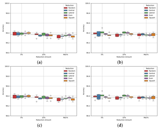
Figure 8.
Experimental results for Site Fazbear test set. (a) Accuracy, Majority class reduced; (b) Accuracy, Both classes reduced; (c) AUC, Majority class reduced; (d) AUC, Both classes reduced.
Figure 8.
Experimental results for Site Fazbear test set. (a) Accuracy, Majority class reduced; (b) Accuracy, Both classes reduced; (c) AUC, Majority class reduced; (d) AUC, Both classes reduced.
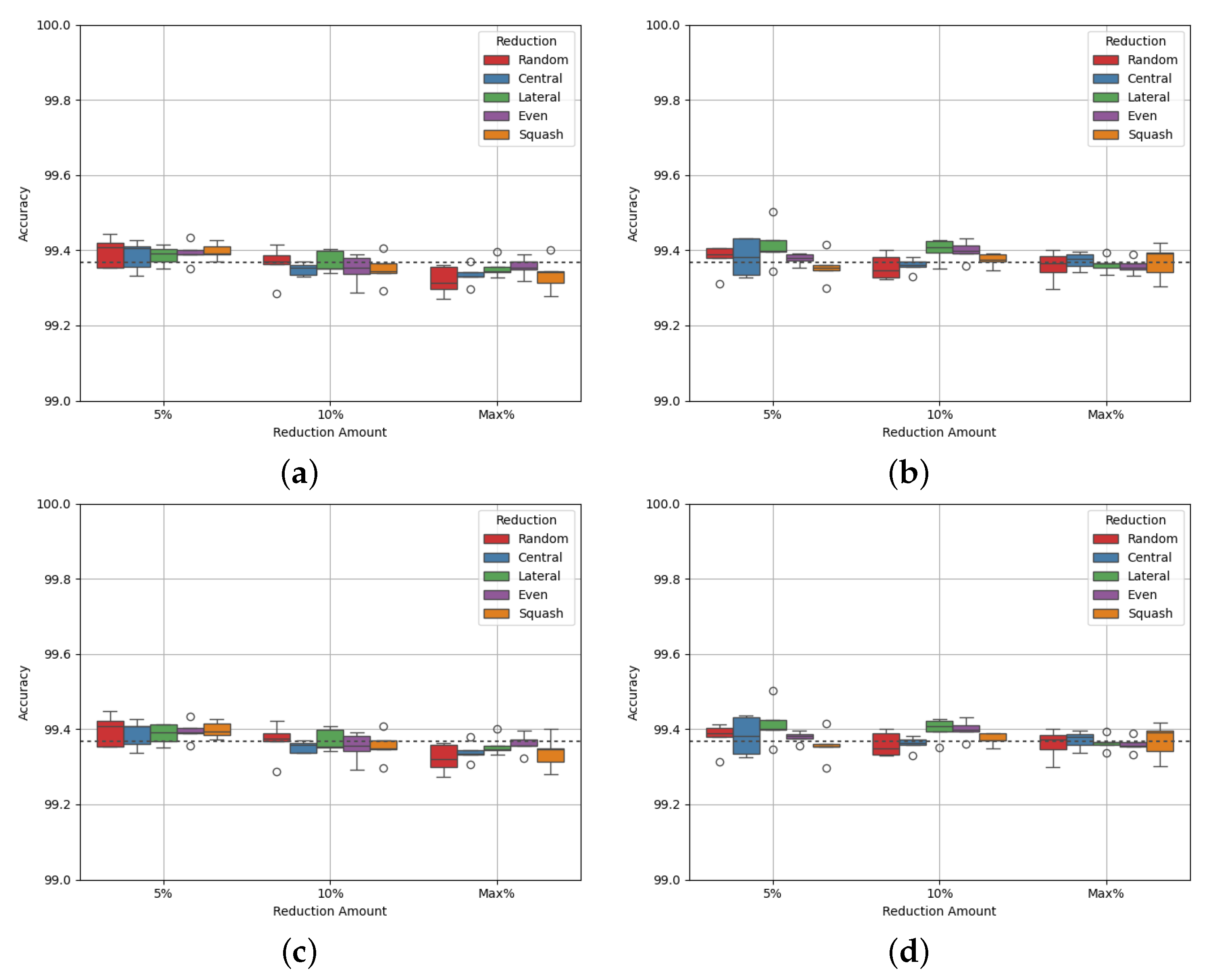
Table 25.
p-values of the AUC metrics of each experiment of reduction on the majority class, on Site Fazbear test set. Values marked with an * have a statistically significant difference from the benchmark.
Table 25.
p-values of the AUC metrics of each experiment of reduction on the majority class, on Site Fazbear test set. Values marked with an * have a statistically significant difference from the benchmark.
| Reduction | Random | Central | Lateral | Even | Squash |
|---|---|---|---|---|---|
| 5% | 0.191 | 0.297 | 0.182 | 0.101 | 3.72 * |
| 10% | 0.993 | 9.94 | 0.834 | 0.435 | 0.489 |
| Max | 6.08 | 7.90 | 0.384 | 0.594 | 0.207 |
Table 26.
p-values of the AUC metrics of each experiment of reduction on both classes, on Site Fazbear test set. Values marked with an * have a statistically significant difference from the benchmark.
Table 26.
p-values of the AUC metrics of each experiment of reduction on both classes, on Site Fazbear test set. Values marked with an * have a statistically significant difference from the benchmark.
| Reduction | Random | Central | Lateral | Even | Squash |
|---|---|---|---|---|---|
| 5% | 0.534 | 0.574 | 0.138 | 0.18 | 0.568 |
| 10% | 0.596 | 0.476 | 6.91 | 5.22 | 0.47 |
| Max | 0.727 | 0.742 | 0.669 | 0.442 | 0.929 |
Table 27.
Class density of Site Fazbear dataset after data reduction on the majority class only. R: random reduction, C: central reduction, L: lateral reduction, E: even reduction, S: squash reduction.
Table 27.
Class density of Site Fazbear dataset after data reduction on the majority class only. R: random reduction, C: central reduction, L: lateral reduction, E: even reduction, S: squash reduction.
| Class 0 (Not Occupied) | Class 1 (Occupied) | |||||||||
|---|---|---|---|---|---|---|---|---|---|---|
| Data Reduced | R | C | L | E | S | R | C | L | E | S |
| 5% | 1.221 | 1.216 | 1.208 | 1.190 | 1.213 | 0.918 | 0.925 | 0.926 | 0.931 | 0.918 |
| 10% | 1.208 | 1.172 | 1.194 | 1.158 | 1.169 | 0.945 | 0.952 | 0.944 | 0.950 | 0.949 |
| Max | 1.174 | 1.163 | 1.153 | 1.154 | 1.151 | 0.956 | 0.958 | 0.966 | 0.952 | 0.959 |
Table 28.
Class density of Site Fazbear dataset after data reduction across both classes. R: random reduction, C: central reduction, L: lateral reduction, E: even reduction, S: squash reduction.
Table 28.
Class density of Site Fazbear dataset after data reduction across both classes. R: random reduction, C: central reduction, L: lateral reduction, E: even reduction, S: squash reduction.
| Class 0 (Not Occupied) | Class 1 (Occupied) | |||||||||
|---|---|---|---|---|---|---|---|---|---|---|
| Data Reduced | R | C | L | E | S | R | C | L | E | S |
| 5% | 1.263 | 1.249 | 1.256 | 1.239 | 1.242 | 0.896 | 0.896 | 0.896 | 0.893 | 0.893 |
| 10% | 1.247 | 1.268 | 1.269 | 1.233 | 1.229 | 0.893 | 0.885 | 0.900 | 0.885 | 0.898 |
| Max | 1.240 | 1.257 | 1.232 | 1.249 | 1.230 | 0.897 | 0.893 | 0.903 | 0.877 | 0.895 |
3.1.8. Discussion—Individual Site Datasets
First, we discuss the performance of each site individually. We have identified that datasets Alpha, Charlie, and Delta show promising results when performing reduction on the majority class. The AUC-ROC may be maintained, so long as class density shifts towards 1 through data reduction. The class densities of sites Beta, Epsilon, and Fazbear do not converge around 1 as the amount of data is reduced, and the AUC-ROC decreases slightly as a result. Site Epsilon has one of the largest class imbalances, but still fails to improve after class balancing through data reduction. This dataset also has the fewest number of datapoints, which may explain the poor performance after data reduction is performed. Therefore, we cannot rely solely on class imbalance as a criterion for data reduction. Instead, class density offers insight into a dataset that might not be immediately apparent. Class density shows more than class imbalance, it also shows whether a dataset has sufficient data for the methods described in this paper. Class density may therefore be considered as a metric that encompasses class balance and sufficient data, and can be used to determine if data reduction is applicable.
Table 29 shows the runtimes for all the experiments. This shows the benefits data reduction may bring to energy and CO2 cost reduction, as runtime, energy use, and CO2 emissions are directly correlated. For most experiments, by increasing the amount of reduction performed, we reduce the runtime. Sites Alpha, Charlie, Delta, and Epsilon have relatively large class imbalance, meaning they remove more data to balance the classes. However, sites Beta and Fazbear have less imbalance, and therefore remove less data. This is especially apparent for Site Fazbear, where in experiments to balance classes, by performing reduction there is an increase in runtime. This is because the overhead of identifying which data to remove takes longer for this site, due to its size, and as so few data are removed, the runtime is similar to that of its benchmark. This is correlated to the fact that experiments that do not balance the classes are in most cases slightly faster, as the datasets do not have to be split between classes before reduction, which is an additional overhead. This shows again that the data reduction strategies introduced in this paper are not applicable to all datasets such as Site Fazbear. It does however show that for datasets such as Site Charlie, the runtime may be nearly halved (from 44 s to 26 s) by reducing with a cap of 50%, which also improves model performance.
Table 29.
Runtimes for experiments on each individual site at each reduction amount for experiments to balance classes and without class balancing. A: Site Alpha, B: Site Beta, C: Site Charlie, D: Site Delta, E: Site Epsilon, F: Site Fazbear.
To identify which data reduction strategy performs best, we must focus on the best-performing scenarios, as they are the most stable and the most useful. We must also consider the statistical significance of the results. For example, Site Alpha maintains performance in AUC-ROC up to 50% reduction, but none of the reduction strategies show significant difference from the benchmark. Therefore, no strategy can definitively be identified as superior. Site Beta has only inferior results to the benchmark. Site Charlie shows an increase in AUC-ROC that is statistically different from the benchmark. With a 50% reduction, the data squash method is performs best. Site Delta has two results that stand out: the data squash method at 10% reduction and the lateral reduction at 25%. The data squash method is superior, with an average increase in AUC-ROC of 0.137%. For Site Epsilon, a 5% lateral reduction performs best, with an average AUC-ROC increase of 0.0301%. For Site Fazbear, a 5% reduction with the data squash method has a better AUC-ROC by an average of 0.0272%. To conclude, the lateral and squash reduction methods are among the best performing.
3.2. Experiments on Fused Dataset
By fusing all of the sites into one large dataset, we may observe the ability of a single model to generalise on multiple different test sets from different environments. We may then see if data reduction will benefit the model further, as it can with the individual site datasets. Table 30 shows the details of the fused dataset. It has over four million datapoints, whereas the largest individual site has just under 330,000.
Table 30.
Fused dataset properties.
Table 31 shows the benchmark results of experimentation on the fused dataset, with no reduction. The model is trained on a fused training set and tested on individual site test sets.
Table 31.
Fused dataset benchmark.
For all sites, the accuracy and AUC-ROC are lower than their non-fused counterparts. For sites Beta and Charlie, the accuracy is substantially lower, by around 25–30%. For sites Alpha, Beta, Delta, and Epsilon, the AUC-ROC is around 30–35% lower. This shows that despite the training sets having more data, the model is unable to classify well. Sites Charlie and Fazbear are the biggest original datasets, meaning that compared to the other sites, they are affected least by the additional data. This may explain why the AUC-ROCs of these two sites are slightly above those of the other sites.
The runtime of training the fused dataset is 51 min. This is a huge increase in runtime from the sub-minute runtime on individual sites; this shows that there is an exponential increase in runtime with the amount of data used. Because of this large runtime, only the maximum reduction was performed to balance the classes, and each experiment was performed only once.
Table 32 shows the properties of the reduced fused dataset. Over half of the majority class was reduced to balance the classes, giving a total dataset reduction of 38.9%.
Table 33 shows the accuracy of the RF model trained on the reduced fused dataset. Table 34 shows the AUC-ROC. Table 35 shows the class densities of the fused dataset after each reduction method.
Table 32.
Reduced fused dataset properties.
Table 32.
Reduced fused dataset properties.
| Number of Datapoints | Balanced Class Reduction | Total Dataset Reduction |
|---|---|---|
| 2,816,518 | 55.972% | 38.864% |
Table 33.
Reduced fused dataset accuracies. Values in bold indicate best-performing reduction strategy.
Table 33.
Reduced fused dataset accuracies. Values in bold indicate best-performing reduction strategy.
| Site | Random | Central | Lateral | Even | Squash |
|---|---|---|---|---|---|
| Alpha | 65.781% | 65.991% | 66.367% | 66.516% | 67.253% |
| Beta | 75.323% | 75.803% | 75.014% | 74.929% | 75.320% |
| Charlie | 67.267% | 67.361% | 67.207% | 67.176% | 67.469% |
| Delta | 66.793% | 66.187% | 66.479% | 67.045% | 66.684% |
| Espilon | 69.228% | 68.611% | 68.387% | 68.777% | 69.090% |
| Fazbear | 87.051% | 87.095% | 86.941% | 86.728% | 87.337% |
Table 34.
Reduced fused dataset AUC-ROC. Values in bold indicate best-performing reduction strategy.
Table 34.
Reduced fused dataset AUC-ROC. Values in bold indicate best-performing reduction strategy.
| Site | Random | Central | Lateral | Even | Squash |
|---|---|---|---|---|---|
| Alpha | 72.403% | 72.648% | 73.022% | 73.028% | 73.546% |
| Beta | 75.904% | 76.346% | 75.626% | 75.445% | 75.834% |
| Charlie | 77.896% | 77.831% | 77.713% | 77.688% | 77.979% |
| Delta | 74.268% | 73.250% | 74.039% | 74.539% | 74.072% |
| Espilon | 73.863% | 73.187% | 72.951% | 73.093% | 73.576% |
| Fazbear | 86.914% | 86.969% | 86.807% | 86.599% | 87.220% |
Table 35.
Class density of reduced fused dataset. R: random reduction, C: central reduction, L: lateral reduction, E: even reduction, S: squash reduction.
Table 35.
Class density of reduced fused dataset. R: random reduction, C: central reduction, L: lateral reduction, E: even reduction, S: squash reduction.
| Class 0 (Not Occupied) | Class 1 (Occupied) | ||||||||
|---|---|---|---|---|---|---|---|---|---|
| R | C | L | E | S | R | C | L | E | S |
| 1.040 | 1.039 | 1.027 | 1.029 | 1.032 | 0.995 | 0.975 | 1.007 | 0.8869 | 0.980 |
The results show that for all sites except Beta and Fazbear, the accuracy decreases further when data are removed. For all sites, accuracy averages around 65–75% except for Site Fazbear, which is 87%. Still, this is worse performance than when trained on the individual training datasets. As for AUC-ROC, performance is increased from the benchmark for all sites except sites Charlie and Fazbear. As these two sites have the highest benchmark AUC-ROC, it is interesting to see that these two sites perform worse after data reduction; this may be because the data reduction is able to remove more training data from these sites, as there are more data to lose.
3.3. Discussion—Fused Dataset
The fused dataset shows poor performance in both the reduced and non-reduced experiments. Not only are the accuracy and AUC-ROC scores inferior to the individually trained models, but the runtime is far longer. Therefore, this methodology is not appropriate for the purpose of energy saving and running on low-compute devices. However, it does give some insight into the importance of using the correct data; despite each site dataset containing the same types of data (temperature, humidity, and VOC), there are differences between sites that mean datasets cannot be fused in this way.
The runtime of training the fused dataset is 51 min, and 28 min for the reduced fused dataset. While there is a significant decrease in runtime by performing this reduction, 28 min is still much larger than the times observed when training the individual datasets, which are all less than 1 min. As they are proportional, this runtime means there is an equivalent increase in energy cost and CO2 usage, which is incompatible with the aim of reducing energy and CO2 cost for moving towards green AI. This shows that using too much data can be detrimental to training in both model performance and cost, despite the similarities between the original data and the additional data.
4. Conclusions
This paper has identified that class density may be used as a metric to qualify a dataset for reduction. The results have shown that for datasets like Site Charlie, which are abundant in data and heavily imbalanced, data reduction on the majority class may be used to improve model performance and reduce the computation required to train the model, due to there being less data. For other datasets like sites Alpha and Delta that are either abundant in data or highly imbalanced, data reduction may be used to at least maintain performance. For highly balanced or less abundant datasets such as sites Beta, Epsilon, and Fazbear, data reduction is not as beneficial. By calculating the class densities of a dataset and gradually reducing the data, if the class densities converge towards a value of 1 then the dataset may be reduced while performance is maintained.
A direction for future work might be to first perform data reduction on each individual site dataset, and then attempt dataset fusion. This should ensure that the most important data are retained at the reduction stage. Alternatively, one might reduce the datasets to a much smaller set, with more data reduction than needed to balance the classes. Dataset fusion on heavily reduced data may contain insightful data that could improve model reliability in new domains.
Author Contributions
Conceptualization, D.S. and T.K.; methodology, D.S.; software, D.S.; validation, D.S; formal analysis, D.S and T.K.; investigation, D.S; resources, D.S; data curation, D.S.; writing—original draft preparation, D.S.; writing—review and editing, T.K.; visualization, D.S.; supervision, T.K.; project administration, T.K.; funding acquisition, T.K. All authors have read and agreed to the published version of the manuscript.
Funding
This research was funded by InnovateUK, project number 10097909.
Institutional Review Board Statement
Not applicable.
Informed Consent Statement
Not applicable.
Data Availability Statement
The open-source dataset used in this study may be found here: https://springernature.figshare.com/collections/A_High-Fidelity_Residential_Building_Occupancy_Detection_Dataset/5364449 (accessed on 16 April 2024).
Acknowledgments
This research performed as part of the D-XPERT AI-Based Recommender System for Smart Energy Saving.
Conflicts of Interest
The authors declare no conflicts of interest.
Abbreviations
The following abbreviations are used in this manuscript:
| HVAC | Heating, ventilation and air conditioning |
| T | Temperature |
| H | Humidity |
| VOC | Volatile organic compound |
| ML | Machine learning |
| AI | Artificial intelligence |
| PCA | Principle component analysis |
| AUC-ROC | Area under the receiver operating characteristic curve |
| RF | Random Forest |
| CNN | Convolutional Neural Network |
| LSTM | Long Short-Term Memory |
| KNN | K-Nearest Neighbour |
| csv | Comma-Separated Value |
References
- Erickson, V.L.; Carreira-Perpinan, M.A.; Cerpa, A.E. OBSERVE: Occupancy-based system for efficient reduction of HVAC energy. In Proceedings of the 10th ACM/IEEE International Conference on Information Processing in Sensor Networks, Chicago, IL, USA, 12–14 April 2011; pp. 258–269. [Google Scholar]
- Ahmad, J.; Masood, F.; Shah, S.A.; Jamal, S.S.; Hussain, I. A Novel Secure Occupancy Monitoring Scheme Based on Multi-Chaos Mapping. Symmetry 2020, 12, 350. [Google Scholar] [CrossRef]
- Krug, S.; O’Nils, M. Modeling and Comparison of Delay and Energy Cost of IoT Data Transfers. IEEE Access 2019, 7, 58654–58675. [Google Scholar] [CrossRef]
- Shafran-Nathan, R.; Levy, I.; Levin, N.; Broday, D.M. Ecological bias in environmental health studies: The problem of aggregation of multiple data sources. Air Qual. Atmos. Health 2017, 10, 411–420. [Google Scholar] [CrossRef]
- Kubat, M. Addressing the Curse of Imbalanced Training Sets: One-Sided Selection. In Proceedings of the Fourteenth International Conference on Machine Learning, Nashville, TN, USA, 8–12 July 1997. [Google Scholar]
- ur Rehman, M.H.; Liew, C.S.; Abbas, A.; Jayaraman, P.P.; Wah, T.Y.; Khan, S.U. Big Data Reduction Methods: A Survey. Data Sci. Eng. 2016, 1, 265–284. [Google Scholar] [CrossRef]
- Schwartz, R.; Dodge, J.; Smith, N.A.; Etzioni, O. Green AI. Commun. ACM 2020, 63, 54–63. [Google Scholar] [CrossRef]
- Whang, S.E.; Roh, Y.; Song, H.; Lee, J.G. Data collection and quality challenges in deep learning: A data-centric AI perspective. VLDB J. 2023, 32, 791–813. [Google Scholar] [CrossRef]
- Kaur, P.; Gosain, A. Comparing the Behavior of Oversampling and Undersampling Approach of Class Imbalance Learning by Combining Class Imbalance Problem with Noise. In ICT Based Innovations; Saini, A.K., Nayak, A.K., Vyas, R.K., Eds.; Springer: Singapore, 2018; pp. 23–30. [Google Scholar]
- Moser, B.B.; Raue, F.; Dengel, A. A Study in Dataset Pruning for Image Super-Resolution. Artif. Neural Netw. Mach. Learn.—ICANN 2024, 9, 351–363. [Google Scholar] [CrossRef]
- Paul, M.; Ganguli, S.; Dziugaite, G.K. Deep Learning on a Data Diet: Finding Important Examples Early in Training. In Proceedings of the 35th Conference on Neural Information Processing Systems (NeurIPS 2021), Online, 6–14 December 2021. [Google Scholar] [CrossRef]
- Toneva, M.; Sordoni, A.; des Combes, R.T.; Trischler, A.; Bengio, Y.; Gordon, G.J. An Empirical Study of Example Forgetting during Deep Neural Network Learning. In Proceedings of the 7th International Conference on Learning Representations, ICLR 2019, New Orleans, LA, USA, 6–9 May 2019. [Google Scholar]
- Bessa, M.; Bostanabad, R.; Liu, Z.; Hu, A.; Apley, D.W.; Brinson, C.; Chen, W.; Liu, W.K. A framework for data-driven analysis of materials under uncertainty: Countering the curse of dimensionality. Comput. Methods Appl. Mech. Eng. 2017, 320, 633–667. [Google Scholar] [CrossRef]
- Ashraf, M.; Anowar, F.; Setu, J.H.; Chowdhury, A.I.; Ahmed, E.; Islam, A.; Al-Mamun, A. A Survey on Dimensionality Reduction Techniques for Time-Series Data. IEEE Access 2023, 11, 42909–42923. [Google Scholar] [CrossRef]
- Ma, J.; Yuan, Y. Dimension reduction of image deep feature using PCA. J. Vis. Commun. Image Represent. 2019, 63, 102578. [Google Scholar] [CrossRef]
- Zaheer, R.; Hanif, M.K.; Sarwar, M.U.; Talib, R. Evaluating the Effectiveness of Dimensionality Reduction on Machine Learning Algorithms in Time Series Forecasting. IEEE Access 2025, 13, 50493–50510. [Google Scholar] [CrossRef]
- Sanderson, D.; Kalganova, T. Dynamic Data Inclusion with Sliding Window. In Proceedings of the Intelligent Sustainable Systems, London, UK, 23–26 July 2024; Nagar, A.K., Jat, D.S., Mishra, D.K., Joshi, A., Eds.; Springer: Singapore, 2024; pp. 525–544. [Google Scholar]
- Byerly, A.; Kalganova, T. Class Density and Dataset Quality in High-Dimensional, Unstructured Data. arXiv 2022, arXiv:2202.03856. [Google Scholar] [CrossRef]
- Sayed, A.N.; Himeur, Y.; Bensaali, F. Deep and transfer learning for building occupancy detection: A review and comparative analysis. Eng. Appl. Artif. Intell. 2022, 115, 105254. [Google Scholar] [CrossRef]
- Chitnis, S.; Somu, N.; Kowli, A. Occupancy estimation with environmental sensors: The possibilities and limitations. Energy Built Environ. 2025, 6, 96–108. [Google Scholar] [CrossRef]
- Zemouri, S.; Gkoufas, Y.; Murphy, J. A Machine Learning Approach to Indoor Occupancy Detection Using Non-Intrusive Environmental Sensor Data. In Proceedings of the 3rd International Conference on Big Data and Internet of Things, Melbourn, VIC, Australia, 22–24 August 2019; Association for Computing Machinery: New York, NY, USA, 2019; pp. 70–74. [Google Scholar] [CrossRef]
- Mohammadabadi, A.; Rahnama, S.; Afshari, A. Indoor Occupancy Detection Based on Environmental Data Using CNN-XGboost Model: Experimental Validation in a Residential Building. Sustainability 2022, 14, 14644. [Google Scholar] [CrossRef]
- Vela, A.; Alvarado-Uribe, J.; Davila, M.; Hernandez-Gress, N.; Ceballos, H.G. Estimating Occupancy Levels in Enclosed Spaces Using Environmental Variables: A Fitness Gym and Living Room as Evaluation Scenarios. Sensors 2020, 20, 6579. [Google Scholar] [CrossRef]
- Pereira, L.M.; Salazar, A.; Vergara, L. On Comparing Early and Late Fusion Methods. In Advances in Computational Intelligence; Rojas, I., Joya, G., Catala, A., Eds.; Springer: Cham, Switzerland, 2023; Volume 14134. [Google Scholar] [CrossRef]
- Tsanousa, A.; Moschou, C.; Bektsis, E.; Vrochidis, S.; Kompatsiaris, I. Fusion of Environmental Sensors for Occupancy Detection in a Real Construction Site. Sensors 2023, 23, 9596. [Google Scholar] [CrossRef]
- Nguyen, T.; Khadka, R.; Phan, N.; Yazidi, A.; Halvorsen, P.; Riegler, M.A. Combining datasets to increase the number of samples and improve model fitting. In Proceedings of the 2023 International Joint Conference on Neural Networks (IJCNN), Gold Coast, Australia, 18–23 June 2023; pp. 1–9. [Google Scholar] [CrossRef]
- Vela, A.; Alvarado-Uribe, J.; Ceballos, H.G. Indoor Environment Dataset to Estimate Room Occupancy. Data 2021, 6, 133. [Google Scholar] [CrossRef]
- Schwee, J.H.; Johansen, A.; Jørgensen, B.N.; Kjærgaard, M.B.; Mattera, C.G.; Sangogboye, F.C.; Veje, C. Room-level occupant counts and environmental quality from heterogeneous sensing modalities in a smart building. Sci. Data 2019, 6, 287. [Google Scholar] [CrossRef]
- Jacoby, M.; Tan, S.Y.; Henze, G.; Sarkar, S. A high-fidelity residential building occupancy detection dataset. Sci. Data 2021, 8, 280. [Google Scholar] [CrossRef]
- Anil Jadhav, D.P.; Ramanathan, K. Comparison of Performance of Data Imputation Methods for Numeric Dataset. Appl. Artif. Intell. 2019, 33, 913–933. [Google Scholar] [CrossRef]
- Filippakis, P.; Ougiaroglou, S.; Evangelidis, G. Prototype Selection for Multilabel Instance-Based Learning. Information 2023, 14, 572. [Google Scholar] [CrossRef]
- Uddin, M.F. Addressing Accuracy Paradox Using Enhanched Weighted Performance Metric in Machine Learning. In Proceedings of the 2019 Sixth HCT Information Technology Trends (ITT), Ras Al Khaimah, United Arab Emirates, 20–21 November 2019; pp. 319–324. [Google Scholar] [CrossRef]
- Bradley, A.P. The use of the area under the ROC curve in the evaluation of machine learning algorithms. Pattern Recognit. 1997, 30, 1145–1159. [Google Scholar] [CrossRef]
- Martin Malík, REALiX, s.r.o. HWiNFO. Available online: https://www.hwinfo.com/ (accessed on 10 April 2025).
- The Department for Energy Security and Net Zero. Greenhouse Gas Reporting: Conversion Factors. 2024. Available online: https://www.gov.uk/government/publications/greenhouse-gas-reporting-conversion-factors-2024 (accessed on 11 April 2024).
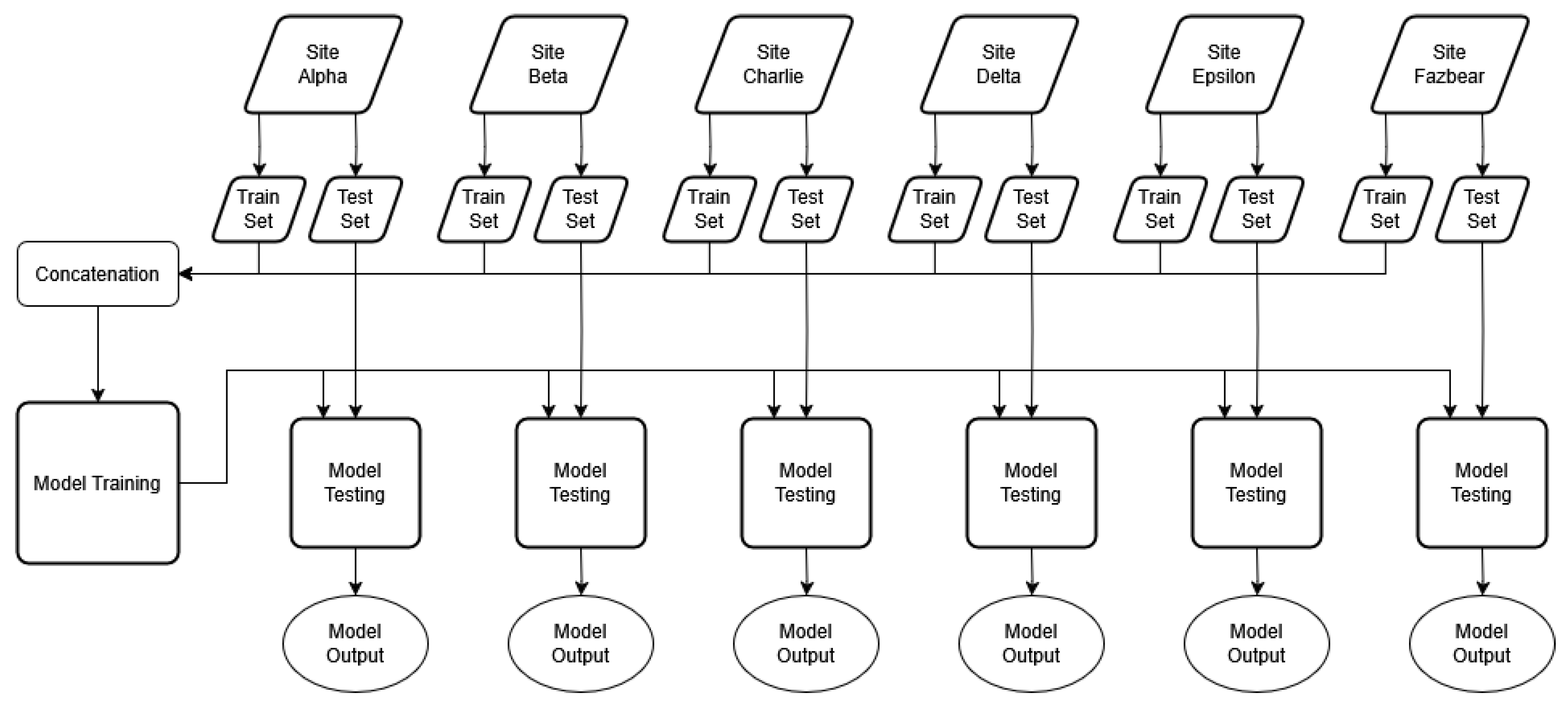
Disclaimer/Publisher’s Note: The statements, opinions and data contained in all publications are solely those of the individual author(s) and contributor(s) and not of MDPI and/or the editor(s). MDPI and/or the editor(s) disclaim responsibility for any injury to people or property resulting from any ideas, methods, instructions or products referred to in the content. |
© 2025 by the authors. Licensee MDPI, Basel, Switzerland. This article is an open access article distributed under the terms and conditions of the Creative Commons Attribution (CC BY) license (https://creativecommons.org/licenses/by/4.0/).