Abstract
Background: Accurate ground segmentation in 3D point clouds is critical for robotic perception, enabling robust navigation, object detection, and environmental mapping. However, existing methods struggle with over-segmentation, under-segmentation, and computational inefficiency, particularly in dynamic or complex environments. Methods: This study proposes FASTSeg3D, a novel two-stage algorithm for real-time ground filtering. First, Range Elevation Estimation (REE) organizes point clouds efficiently while filtering outliers. Second, adaptive Window-Based Model Fitting (WBMF) addresses over-segmentation by dynamically adjusting to local geometric features. The method was rigorously evaluated in four challenging scenarios: large objects (vehicles), pedestrians, small debris/vegetation, and rainy conditions across day/night cycles. Results: FASTSeg3D achieved state-of-the-art performance, with a mean error of <7%, error sensitivity < 10%, and IoU scores > 90% in all scenarios except extreme cases (rainy/night small-object conditions). It maintained a processing speed 10× faster than comparable methods, enabling real-time operation. The algorithm also outperformed benchmarks in F1 score (avg. 94.2%) and kappa coefficient (avg. 0.91), demonstrating superior robustness. Conclusions: FASTSeg3D addresses critical limitations in ground segmentation by balancing speed and accuracy, making it ideal for real-time robotic applications in diverse environments. Its computational efficiency and adaptability to edge cases represent a significant advancement for autonomous systems.
1. Introduction
Perception is a vital step toward automation in robotic devices. With growing interest in autonomous systems, safety and efficiency remain paramount [1]. A key component of effective perception tasks for robotic devices is obtaining accurate orientation and depth information about their surroundings. Therefore, many applications—such as scene registration and reconstruction (for reverse engineering), simultaneous localization and mapping (SLAM) for autonomous navigation and control, and three-dimensional (3D) object detection—require sensors that can collect 3D and depth information to complete tasks successfully and efficiently.
Although recent research trends have explored depth estimation using monocular cameras, this approach is inherently challenging [2,3] and its depth estimation accuracy over a distance is still inferior compared to sensors that can directly capture high-precision point clouds with rich and reliable environmental information for processing and interpretation by robots.
The mobile Light Detection and Ranging (LiDAR) sensor, also referred to as the mobile laser scanner (MLS), is a common sensor of choice for autonomous navigation systems (robots) to capture 3D point cloud information for perception tasks. With a point density or resolution greater than 100 pts/m2 and a shorter survey distance, the MLS point cloud offers rich and reliable information about the environment [4,5]. However, these point clouds are usually unstructured, sparse, noisy, and have uneven sampling density. Therefore, ground filtering of point clouds is a crucial preprocessing step in autonomous robot perception systems, and its performance has a strong influence on the overall performance of the perception system. Nevertheless, ground filtering generally suffers from over-segmentation, under-segmentation, or slow segmentation, making it a non-trivial task [6,7,8].
Given these problems, this study proposes a fast ground filtering technique called FASTSeg3D, as presented in Figure 1. A two-stage ground filtering process is performed to extract candidate ground point clouds using a fast point representation technique to quickly organize, downsample, and filter outlier points in the point cloud simultaneously. A sliding-window model fitting approach is used in the second stage to address the over-segmentation problem adaptively, making it robust enough for complex terrains while still achieving real-time filtering. The main contributions of the study are summarized as follows:
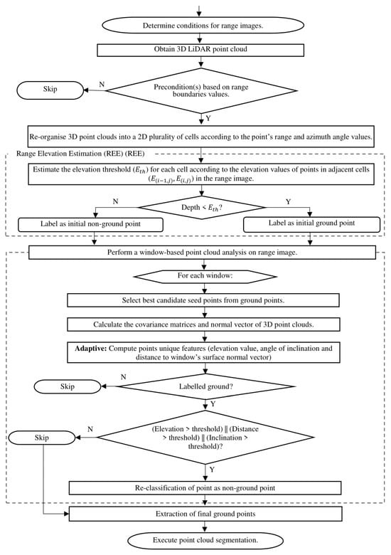
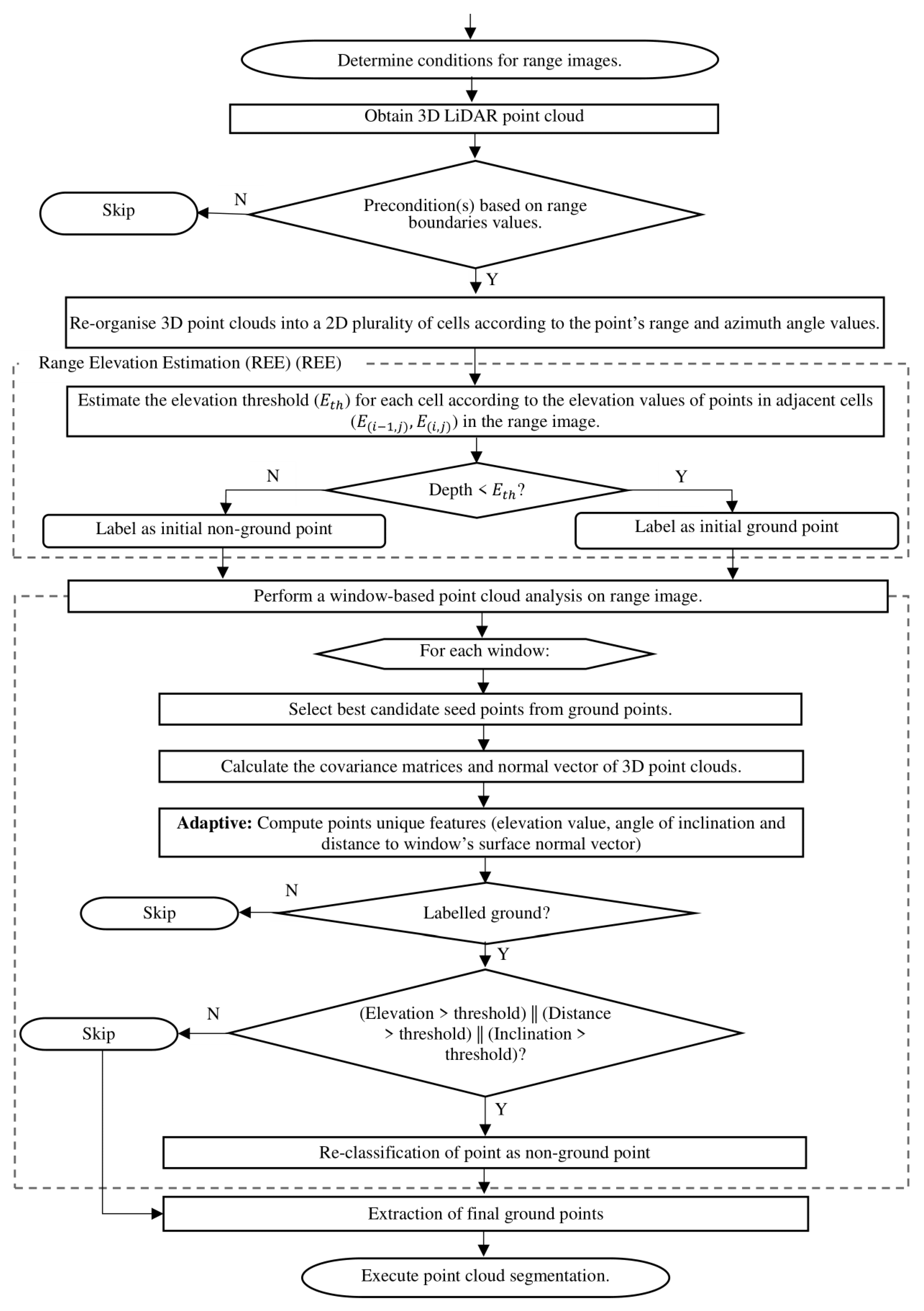
Figure 1.
Flow chart for FastSeg3D Algorithm.
- A range elevation estimation (REE) technique for fast organization of 3D point clouds, filtering of outliers, and estimation of terrain heights
- A window-based model fitting (WBMF) technique to adaptively address the over-segmentation problem and greatly reduce the number of false-positive segmented regions without compromising real-time filtering.
- A fast and adaptable ground filtering/segmentation algorithm (FASTSeg3D) for efficient organization, filtering/segmentation of ground and non-ground points within 3D point clouds in real time.
2. Related Works
To be an effective preprocessing step, the ground filtering/segmentation technique has to be sufficiently fast, efficient, and robust. Unlike supervised approaches that involve learned parameters and lots of training, point cloud segmentation algorithms (including unsupervised clustering algorithms) are fundamentally the results of geometric constraints and statistical rules [8,9,10,11]. These algorithms generally have a well-defined approach towards segmenting regions and are interpretable and reusable. Also, they do not need to be retrained or relabelled to improve accuracy [11,12]. These attributes make them more data efficient than deep learning approaches. Although deep learning approaches are very efficient for applications that do not require real-time usage or have limited memory, point cloud filtering/segmentation algorithms are still a very common choice for applications that require real-time usage or fast preprocessing for downstream applications [13,14,15].
Several traditional techniques have been proposed for ground filtering/segmentation. These techniques are commonly utilized to establish ground planes for Digital Terrain Models (DTM) and Digital Surface Models (DSM) and aim to model and analyse terrain features by fitting ground models to the point cloud data. Various techniques have been employed, including ground filtering based on the construction of surface models, elevation differences, or morphological operations (i.e., erosion, dilation, opening and closing) [11,16,17].
2.1. Reference Ground Surface Filtering
Ground filtering based on a ground surface constructs a reference surface function and then classifies points by their spatial distance from the reference surface. This process is sometimes referred to as plane or ground fitting, or surface-based filtering [18,19]. Typically, a set of ground seed points is selected using specific criteria and gradually refined using various techniques to establish the reference surface function. The criteria for selecting ground seed points can include random selection [19], mean elevation values [20,21,22], or local lowest points [23,24]. The random sample consensus (RANSAC) plane segmentation method, proposed by [19], is one of the earliest approaches for selecting seed ground points and remains effective for flat roads with distinct boundaries. In this method, a minimal subset of data points is randomly selected, and a plane or surface model is fitted to these points. This process is repeated using regression techniques until a surface model with the highest number of inliers is obtained. Due to its fast and robust nature, many variations of RANSAC have been proposed for ground filtering [25,26,27]. However, a common drawback of these methods is their performance on curved or uneven terrains.
Some researchers proposed alternative regression techniques to address this problem [18,28,29,30]. Refs. [18,28] suggested using Gaussian process regression (GPR) to segment point clouds into multiple one-dimensional (1D) GPR problems with a covariance function, aiming to reduce complexity and improve computational efficiency. However, this method struggles on steep slopes and does not guarantee continuity in overall ground elevation. Ref. [29] proposed a more complex regression technique to accurately estimate ground heights. That approach integrated GPR with robust locally weighted regression (RLWR) to form a hybrid regression model, which proved to be robust in estimating road surfaces. Nevertheless, the success of that method depended on the accurate selection of pavement seed points, and it was more computationally demanding compared to GPR alone. Ref. [30] divided the ground surface into even segments and applied the region-growing clustering algorithm to the initial seed ground points for each segment. The approach aimed to segment the ground planes according to a specific distance threshold.
Ref. [20] constructed a reference ground surface model by interpolating initial seed points selected based on their mean elevation values. The reference ground surface was iteratively refined by assigning appropriate weights to each point. Ref. [31] improved that concept by introducing a hierarchical or multi-scale interpolation approach, allowing for data processing at multiple resolutions. Ref. [32] proposed the multi-scale curvature classification (MCC) method, which employed thin plate spline (TPS) interpolation to generate a reference ground surface from the seed points. The MCC method is simple and requires minimal user-defined parameters, such as initial scale and curvature tolerance. While MCC is highly effective in complex vegetation terrains, it struggles in very dense areas and regions with steep slopes, leading to misclassification of points. Its accuracy can also be influenced by the choice of parameters. Researchers have since proposed improvements to the MCC algorithm, such as the parameter-free hierarchical TPS interpolation by [33], enhanced smoothing TPS between adjacent levels by [34], and saliency-aware TPS interpolation for a terrain-adaptive ground filtering method by [35].
Ref. [36] used the moving-window weighted iterative least-squares fitting method to select seed points and applied the region-growing method [37,38] to reconstruct the complete set of ground points. Another approach to seed point selection for surface fitting or filtering is the progressive triangulated irregular network (TIN) densification filtering (PTDF) approach introduced by [23], which selects the lowest points as seed points. Although many improvements have been proposed to address the time consumption issue in the PTDF approach [24,39,40,41], PTDF variants still struggle to retain ground points in steep regions and may suffer from misclassification of ground points as non-ground due to the seed point selection strategy.
Reference ground surface models can also be established using active shape models. Ref. [42] proposed an algorithm utilizing an active shape model that behaved like a rubber cloth with elasticity and rigidity to estimate the ground surface. The surface shape was controlled by an energy function that minimized the energy to determine the surface position in a parametric form. Ref. [43] introduced the Cloth Simulation Filtering (CSF) method, an easy-to-use, fast, and efficient algorithm for ground filtering. The input LiDAR point cloud data were inverted, and a rigid cloth of a set resolution was used to cover the inverted surface, simulating the behaviour of a physical membrane. The interactions between cloth nodes and LiDAR points were analysed to determine the positions of the cloth nodes and approximate the reference ground surface. Finally, ground points were extracted by comparing the original LiDAR points with the generated surface. While this approach was efficient and adaptable to different terrains [43,44,45,46], it was still prone to environmental noise and struggled with complex terrains with steep slopes and large variability.
2.2. Elevation Differences Filtering
Slope or elevation ground filtering extracts ground points based on the slope differences between two points. This concept was introduced by [47], who assessed the local maximum slope and the elevation difference of the landscape. This approach is fast and effective when applied to fused point clouds built from multiple 3D scans but suffers from overfitting and is unsuitable for complex terrains. Many researchers have proposed improvements to adapt this approach to more complex terrain [48,49,50]. Ref. [49] proposed an adaptive method that automatically updated the slope threshold after each iteration. To address errors due to directional sensitivity, ref. [48] proposed the Multi-directional Ground Filtering (MGF) algorithm, which incorporated a two-dimensional neighbourhood in directional scanning. Ref. [50] applied a slope-based filter to each profile of LiDAR points in one direction and another filter to the same profile in the opposite direction (180 degrees apart) to address over-filtering, especially in cliff-like terrains. However, that approach was parameter-sensitive and computationally demanding.
Ref. [51] adopted that approach to propose the elevation map method. Initially introduced by researchers at Stanford University, the algorithm segments the point cloud into cells and calculates the maximum height difference within each cell. If the difference surpasses a certain threshold, all points in the cell are classified as non-ground points. Although this straightforward method can manage irregular terrains, it may lead to incorrect classifications in cells with a sparse number of points or those containing overhanging structures. Ref. [52] proposed using a multi-volume grid elevation map to store the start and end heights of the consistent vertical regions in each cell, tracking the ground planes. However, their solution did not focus on coarse-to-fine ground segmentation and was insensitive to slope terrain.
The slope and elevation map ground filtering method demonstrates the potential for establishing distinct geometric features for ground filtering [53,54]. This is also explored in Conditional Random Field (CRF) methods, like the Markov Random Field (MRF) method, which uses gradient cues of the road geometry to implement belief propagation for classifying the robot’s environment into different regions [55,56]. While this approach has proven robust on uneven terrain, it is time-consuming.
2.3. Morphological Operations Filtering
Some researchers apply morphological operations to point cloud data (PCD) for ground filtering. These non-linear operations are used to expand or reduce certain object sizes [57,58,59]. This concept was applied by [60] to PCD for ground filtering, but it was ineffective in filtering large-sized objects. To address this, ref. [61] proposed progressive morphological filters (PMFs), which gradually increased the window size to accommodate larger objects. Ref. [62] suggested adapting the algorithm to different terrains without the need for constant-slope assumptions. Due to the computational demands of PMFs, ref. [63] proposed the simple morphological filter (SMRF), which employed a linear increase in window size and a slope thresholding technique to filter objects. Ref. [64] introduced the use of differential morphological profiles (DMPs) on points’ residuals from the approximated surface, forming a top-hat scale space to extract ground points based on their geometric attributes. Many other researchers have proposed methods to enhance the effectiveness of morphological filters (MFs) in complex terrains [64,65,66,67,68]. However, MFs are less effective for complex structures and varying object sizes and may become computationally expensive when performance improvements are sought.
3. Methods
3.1. Problem Definition
For a given 3D point with Cartesian coordinates , in a 3D LiDAR point cloud , where and P contain N points, the task is to estimate the number of points in P, with guaranteed recall and precision performance, that can be classified as a ground class, including relatively flat [69] surfaces like drivable surfaces, terrain, pavements, and other flat surfaces or a non-ground class, which includes vehicles, humans, and static and movable objects.
3.2. FastSeg3D: Point Cloud Data Representation
To estimate the elevation of each point in the 2D map, the range elevation estimation (REE) technique was proposed. Ideally, the lowest (sets of) height(s) within a given grid cell of a point cloud are expected to be ground points, and it is based on this assumption that elevation features are extracted and height thresholds are determined. But this is not always the case. For instance, some grids do not contain ground points, road and drivable terrains are not always flat, and occasionally, noisy points are observed below the ground points as a result of reflected points from objects and this can lead to under-segmentation. To address noisy points, refs. [70,71] observed that noisy points usually contained a noticeably smaller intensity as compared to their neighbouring points and the authors proposed intensity correction techniques to address the effect of noisy points on lane detection and improve the simultaneous localization and mapping (SLAM) framework, respectively. Also, the incidence angle () of each point affects the intensity of each point. Ref. [72] conducted some analysis on the impact of the incidence angle on intensity and reported that reflectance was proportional to the incidence angle. This also explained the relatively smaller intensity of noisy points.
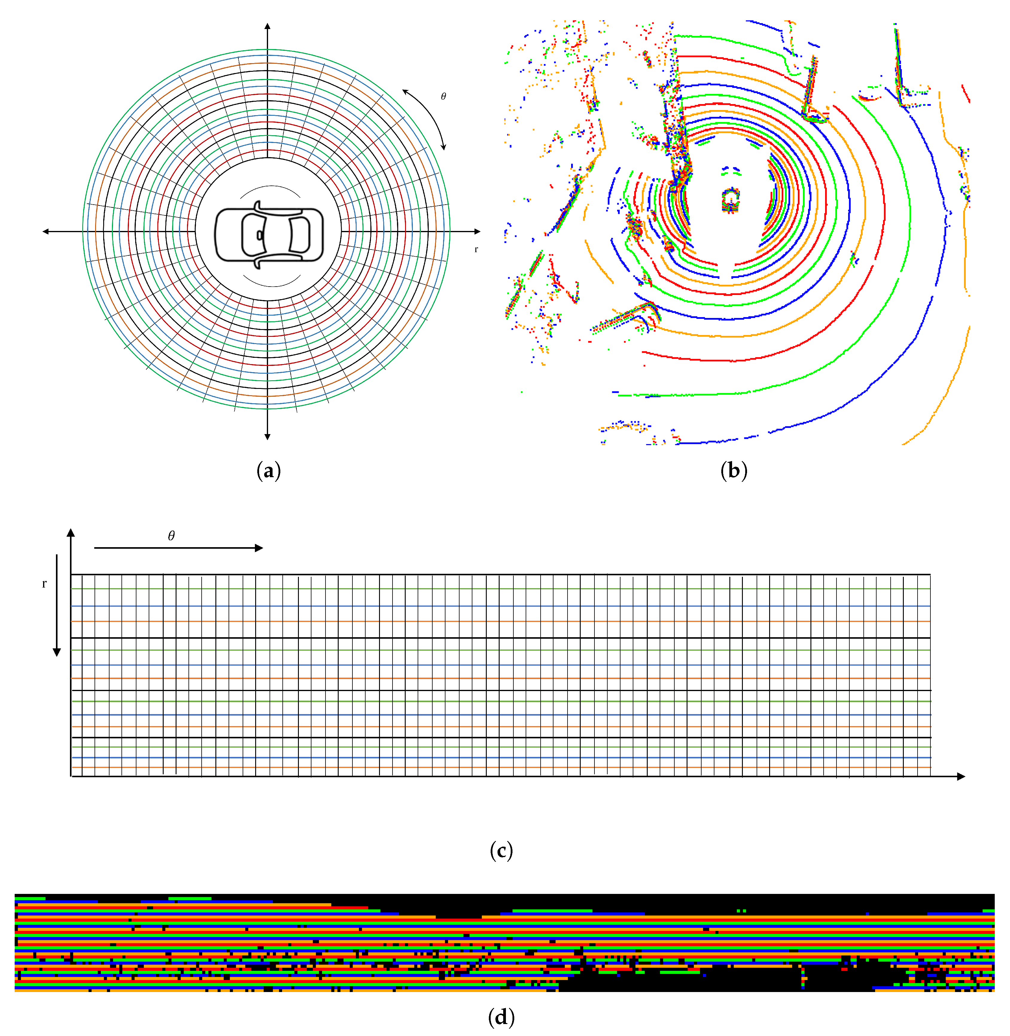
Since the 2D range image representation technique has demonstrated its performance, effectiveness in point distribution over varying distances and inexpensive computational cost for point cloud representation, like the ring elevation map [73] and the polar grid technique [29], the FastSeg3D employs similar data representation method, as shown in Figure 2, to achieving a fast means of organising the raw captured point clouds. The range values and azimuthal angle (horizontal angles) of each point in the point cloud, P is used to represent all points as a 2D image .
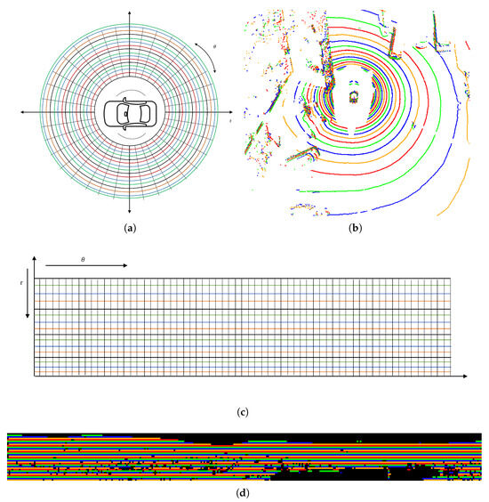
Figure 2.
Point cloud representation; (a) graphical representation of the distribution of points in a point cloud according to its spatial information; (b) data image as captured from the cloud viewer, with each color representing a different laser beam number, for presentation purpose; (c) 2D range image representation of the point cloud; (d) point cloud data representation as captured in C++ using the PCL and OpenCV libraries, for presentation purpose.
To achieve this, an empty placeholder 2D image is created, and a data structure is also created for fast lookup, where the attributes in the data structure are the unique features of every point in the point cloud: cloud index , point labels , elevation value , distance of point to origin , and inclination angle . The range value and azimuthal angle values for a given point in the point cloud, P can be expressed as:
where:
The maximum row range of the 2D image is determined by the approximate maximum range of accurate measurements from most common LiDAR systems like the Velodyne 32E, and 64E, used by autonomous robots. This value is usually around 70 m, therefore the range of values for the row of the 2D image, which represents the range values of each point in the point cloud, was set to 0–70 m. The maximum column range of the 2D image is determined by using the rated angular resolution (horizontal/azimuth) of the LiDAR datasheet, which is between the range of to . Since the LiDAR sensor/system performs a scan, it is divided by the resolution to estimate the maximum column range, that is, , which gives a value of 900. Now, the best case, which is , gives a value of 3600, but this is only possible if the LiDAR system is run at a very low RPM of about 300, which is not ideal for capturing point clouds in real time. Most LiDAR systems used for navigational purposes are configured to run at maximum speed (approximately 20 Hz) with an RPM of about 1200, which accounts for the angular resolution of . With a calculated value of 900, the formula is used to find the closest value to but greater than 900 to ensure that the image representation of the point cloud conforms with the standard computer vision resolution for images. Therefore, the maximum column value was set to 1024 for 32-beam laser LiDAR and 2048 for 64-beam laser LiDAR systems.
Every point in the point cloud is allocated to a cell/pixel in the 2D image once its calculated values fall within the 2D range image. The angular resolution for each cell of the 2D range image can be obtained from the LiDAR field of view (FOV); this could be divided by the maximum column value (this could be 1024 or 2048). Additionally, the vertical resolution can be obtained from the range values, which were set to 70 m divided by the LiDAR number of lasers. For instance, the Velodyne 32E has 32 laser scanners and the Velodyne 64E has 64. Points that fall within the range of 0–2 m are filtered out to account for points that fall on the ego vehicle during the LiDAR system scan. This condition can be expressed as follows:
3.3. Algorithm 1: Range Elevation Estimation (REE)
After allocating points to the 2D range image the minimum elevation values and the elevation thresholds of each cell/pixel in the point cloud are estimated and used to determine the ground and non-ground points from all valid points in the 2D range image. Traversing across adjacent points, i.e., across the columns in the 2D range image, the minimum elevation, , is determined by comparing the third spatial coordinate value of the previous point, and the current point, , to find the minimum value. This value is set as the minimum value for the current cell or pixel.
The elevation values are calculated using the coordinate of each point in the point cloud and an elevation tolerance of m along the row, which is also called the adjacent points of the range image. The elevation tolerance is allowed enough tolerance to accommodate all possible ground points during the first segmentation process. For the condition , where the row number is zero, the elevation value is the same as the minimum third spatial coordinate of the point(s) in the current cell/pixel. This can be expressed as:
The REE algorithm is shown in Algorithm 1.
Using the set elevation threshold and the estimated minimum elevation for each cell , a threshold value is set for each cell and used to segment points in that cell as a ground or non-ground point. Therefore, points equal to or above the threshold value are labelled as non-ground points, and points below as ground points. This is expressed as:
The complexity of the REE algorithm is shown in Appendix A.1.
| Algorithm 1 Coarse segmentation (REE) |
| Input: raw point cloud |
| Output: coarsely segmented ground/non-ground labels |
| Parameters: |
| i. : elevation tolerance (default: ) |
| ii. : maximum LiDAR range (default: ) |
| iii. Angular resolution |
| 1: Initialize 2D range image with dimensions |
| 2: for each in cloud P do |
| 3: Compute range ; |
| 4: Compute azimuth ; |
| 5: Map to cell in ; |
| 6: end for |
| 7: for each row r in do |
| 8: Compute minimum elevation ; |
| 9: ; |
| 10: if then |
| 11: ; |
| 12: else |
| 13: ; |
| 14: end if |
| 15: Label points in cell ; |
| 16: if ; then |
| 17: label as non-ground: ; |
| 18: else |
| 19: label as ground: ; |
| 20: end if |
| 21: end for |
| 22: Return labelled point cloud; |
3.4. Algorithm 2: Window-Based Model Fitting (WBMF)
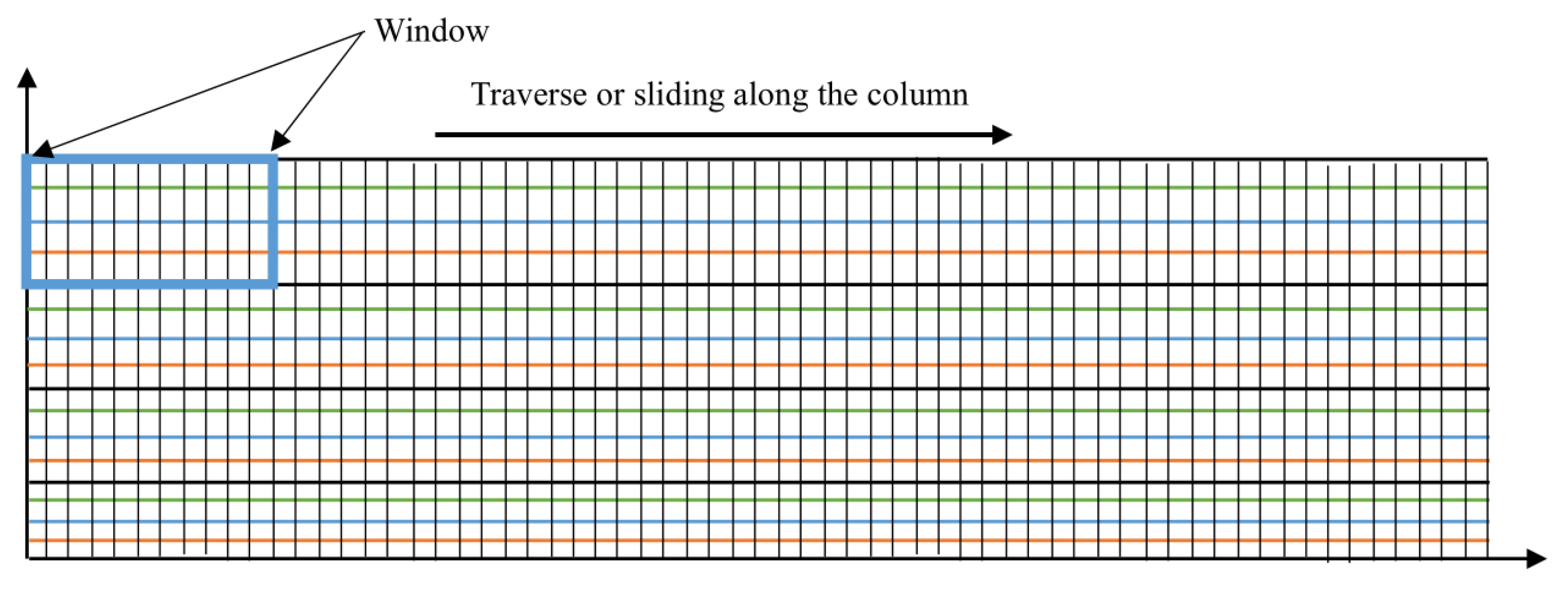
The REE coarse segmentation techniques result in a high level of over-segmentation of ground points, as observed in Figure 3. This is understandable because all valid points within the range image are labelled as ground points before the elevation threshold is used to segment non-ground points. To address this, the window-based model fitting technique is employed to adaptively calculate the unique spatial and geometric features of each point in a predefined region/window size which is a subsection of the entire range image, as shown in Figure 4 and Algorithm 2. This window is traversed across the column, and the spatial and geometric features for each point within the current window are re-calculated. These values are updated in the data structure and used to perform a fine-grain segmentation of the initially segmented points in the point cloud.
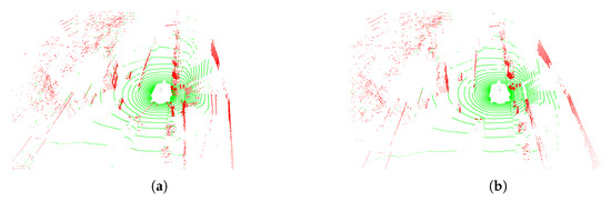
Figure 3.
FASTSEG3D: (a) The image before applying window-based model fitting (WBMF), which exhibits false positives. Green points represent ground points, while red points denote non-ground points; (b) result after the WBMF is applied to address false positives.
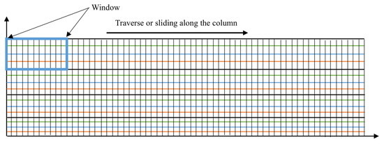
Figure 4.
The window-based model fitting technique.
The 2D image is divided into smaller regions by calculating the subset region dimension, which is depicted as , as shown in Appendix A.2. This is also referred to as the window dimension. The best seed points are determined and used for the plane model and the normal vector using the principal component analysis (PCA) [74] technique. Details are shown in Appendix A.2.
| Algorithm 2 Window-based model fitting (WBMF) |
| Input: coarsely labelled point cloud from REE image, |
| Output: refined ground/non-ground labels |
| Parameters: |
| i. W: window size |
| ii. : elevation tolerance (default: ) |
| iii. Window dimensions , (for grid) |
| iv. Slope threshold , distance threshold , elevation threshold |
| v. Min/max seed points per window: |
| vi. : candidate ground points, where k represents candidate points for |
| vii. NOTE: 0 indicates ground label, and 1 indicates non-ground. |
| 1: Divide 2D range image into sliding windows of size |
| 2: for each window in do |
| 3: Select candidate ground seeds with lowest elevation in |
| 4: Compute covariance matrix M of : |
| 5: , where |
| 6: Perform PCA on M to compute normal vector |
| 7: if then |
| 8: for each point in do |
| 9: Compute distance to plane: |
| 10: Compute inclination angle: |
| 11: if OR OR then |
| 12: Reclassify as non-ground: |
| 13: end if |
| 14: end for |
| 15: else |
| 16: add to |
| 17: end if |
| 18: end for |
| 19: Return refined labels |
4. Results and Discussion
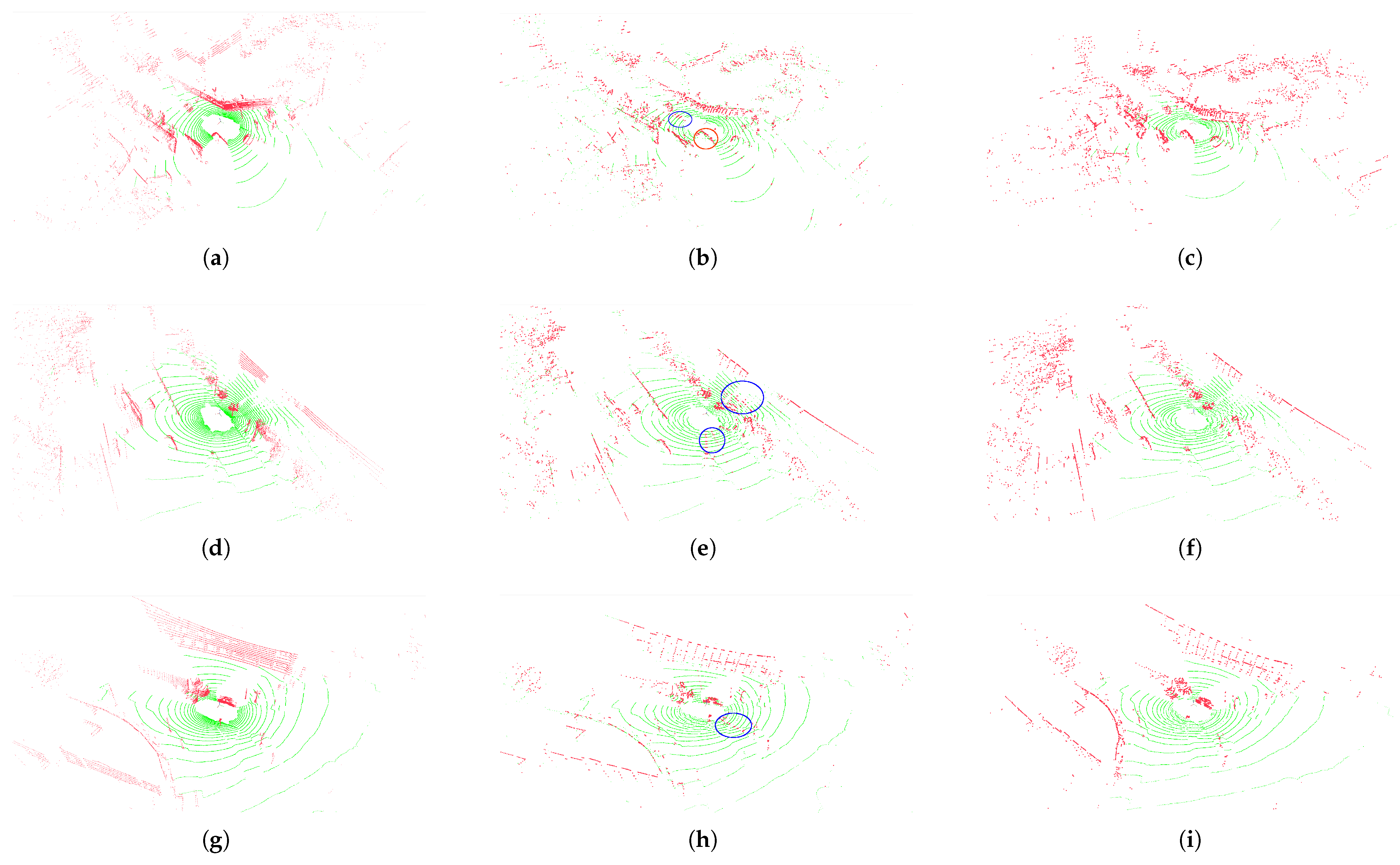
To validate the study’s contribution and verify the progressiveness of both modules (REE, and WBMF), in this section, the performance increase is presented with the introduction of each module and the accuracy-to-speed tradeoff. Then, FASTSEG3D is compared to some existing methods like the CSF [43], RANSAC [19], PTDF [23], and more similar and recent works by [75,76]. Demonstrations of the FASTSEG3D modules alongside the ground truth are shown in Figure 5.
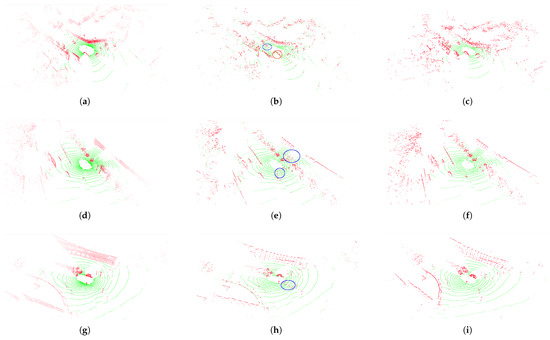
Figure 5.
Qualitative comparison between FASTSEG3D before WBMF (REE) and after WBMF, alongside the ground truth, for ground removal. Three nuScenes samples were selected to demonstrate each algorithm’s performance on uneven terrain. Subfigures (a–c) show the ground truth, REE, and WBMF ground removal results for Sample 1, respectively; subfigures (d–f) depict those for Sample 2; and subfigures (g–i) illustrate those for Sample 3. The REE regions circled in blue indicate false negatives (FNs), where ground points were incorrectly classified as non-ground. The regions circled in red indicate false positives (FPs), where non-ground points were incorrectly classified as ground.
4.1. Experimental Setup
The experiment for all algorithms was performed on the C++ Point Cloud Library (PCL) using the same computer (Ryzen 9 5900x and 32 GB of RAM) for consistency. Then, the NuScenes [77] dataset was adopted to evaluate and compare the proposed FASTSEG3D ground removal algorithm to other efficient algorithms. Based on the point-wise labels, the points labelled as flat.terrain, flat.other, flat.sidewalk, and flat.driveable [77] were considered to be ground points, points labelled as noise were ignored, and every other point was considered to be a non-ground point.
4.2. Experimental Parameters
To conduct the experiments, the following settings were used: the range image dimensions were configured as for the nuScenes dataset. Elevation tolerance was set to .
For WBMF, the window dimensions were defined by rows () and columns (), with and . The number of seed points per window was constrained between a minimum of 5 and a maximum of 20. Additional thresholds included a distance threshold to the window origin , inclination angle threshold , and elevation threshold .
4.3. Evaluation Metrics
To evaluate the proposed approach, the mean error sensitivity ( and ), frames per second (), the mean intersection over union ( and ), the harmonic mean of precision and recall ( and ), the mean kappa coefficient (), and the mean accuracy () for predicted ground and non-ground points in each scene were calculated [11,78,79,80]. The harmonic mean of precision and recall measures the balance between the precision and recall, and the kappa coefficient assesses the reliability of the classification method.
To assess the performance of the proposed algorithm in varying scenarios, the algorithm was tested under different conditions. These conditions included varying lighting (day and night), scenes with predominantly large objects such as vehicles in heavy or dense traffic (), scenes with predominantly pedestrians in heavy or dense traffic (), heavy and fast-moving traffic with lots of objects in rainy, cloudy weather (), and scenes with predominantly small objects (), like vegetation, debris, and traffic cones in heavy or dense traffic. The total numbers of object points and ground points for each scene are presented in Table 1. The total number of object points in each scene explains the rationale behind their selection.

Table 1.
Total numbers of object points and ground points for each scene.
A total of eight scenes were selected based on these conditions from the nuScene LiDAR dataset with a total of 313 LiDAR scan samples. The metrics used can be expressed as:
where represents the number of true positives, true negatives, false negatives, and false positives for predicted points, and represents the recall and precision for ground points, and and represents the recall and precision for non-ground points; represents the observed agreement, and represents the expected agreement by chance.
These metrics give an in-depth insight into how reliable and robust a classification method is for ground filtering. For autonomous driving, these metrics are important to measure the ability of the proposed algorithm to correctly and reliably identify all relevant instances of a target class within a dataset.
The FASTSEG3D modular evaluation begins by showing the performance-to-speed tradeoff in Table 2 for day scenarios and Table 3, for night scenarios. Generally, metric values above 80% and error values below 10% are considered very good scores for prediction. The range values show the spread between the best and worst metrics for the samples of a given scene. The smaller the spread, the better the method.
Table 2.
Performance metrics for different FastSeg3D modules across scenarios (day).
Table 3.
Performance metrics for different FastSeg3D modules across scenarios (night).
Similar to the point cloud 2D image representation of [73], the range elevation map representation of point clouds addresses the limitations of the traditional polar representation for uneven distribution of points over distance. This becomes the premise for the success of the REE technique. Capitalizing on the evenly distributed point cloud to estimate ground points, which are expected to be all points less than the point with the minimum elevation and a certain slope threshold for all points with similar ranges, the REE successfully achieved a rough segmentation. However, the REE module had limited accuracy for ground removal because its threshold for elevation was fixed. This led to a high number of false positives and false negatives as shown in Table 2 and Table 3. These were most obvious in the accuracy and kappa coefficient metrics. In particular, the kappa coefficient for both day and night revealed the reliability or the level of agreement by chance of the REE module.
The WBMF technique takes advantage of the initially classified points of the REE module to refine the initial segmentation. Because points within a similar range could include flat terrains that are above the slope threshold, calculating the surface normal of that region and refining the labels according to the surface normal threshold values for that region was successful, as shown in Figure 5.
4.4. Comparative Methods
The proposed method, FASTSEG3D, was compared with three well-known filtering algorithms and two more recent algorithms, including Cloth Simulation Filtering (CSF) by [43], random sample consensus (RANSAC) by [19], Progressive Triangulated Irregular Network (TIN) Densification Filtering (PTDF) by [23], and more recent works by [75,76]. All algorithms were tested using the same experimental setup as shown in Table 4.
Table 4.
Parameters for compared methods.
For a fair comparison, the parameter setups for all baseline methods were configured according to their original implementations or recommendations. These included CSF, RANSAC, PTDF, PatchWork++, and JPC, as detailed in Table 4. Each method was either tuned via default settings, validation-based optimization, or author-provided configurations to ensure consistency and reproducibility across evaluations.
RANSAC and PTDF were implemented using the PCL [81] and Fade2.5D [82] library, and CSF [43,75,76] was implemented using the publicly available C++ codes (CSF https://github.com/jianboqi/CSF, PatchWork++ https://github.com/url-kaist/patchwork-plusplus, JPC https://github.com/wangx1996/Fast-Ground-Segmentation-Based-on-JPC accessed on 25 April 2022), respectively. Table 5, for the day scenarios, and Table 6, for the night scenarios, show the performance and speed of each algorithm as compared to FASTSG3D.
Table 5.
Performance-to-speed comparison of FASTSEG3D against other algorithms (day).
Table 6.
Performance-to-speed comparison of FASTSEG3D against other algorithms (night).
The result demonstrated that the proposed ground filtering method, FASTSEG3D, performed excellently in segmenting the ground and non-ground points of the given dataset. When all samples were observed, FASTSEG3D was able to achieve an error sensitivity rate for both ground and non-ground points ( and ) of a mean error of less than 7% across all scenarios and an error value of 10% or less across all samples for every scenario for both the day and night test conditions, except for values for the rainy-scene night condition.
Comparatively, refs. [19,76] achieved similar performance for only the mean day test condition. Ref. [43] achieved this for the mean day and night test conditions. However, there were a few outlier results that gave some erroneous values across all samples for the day test condition for the big-object scenario; this can be seen from its range value of 53.30. Ref. [75] only achieved similar results for the mean day and night test conditions. Although [75] performed better than FastSeg3D in the rainy night scenario, FASTSEG3D outperformed [75] by executing its segmentation approximately 10 times faster. The proposed algorithm also demonstrated consistently better IoU scores for both ground and non-ground points across all test conditions maintaining a mean IoU score of above 90% except for the small-object and rainy-weather night conditions.
From Table 6, the rainy and small-object scenarios showed that all methods struggled in the ground filtering task, and this was also observed in the kappa coefficient values. This may be as a result of two key factors:
- LiDAR sensor noise: Rain droplets introduce false returns, increasing outliers below the true ground elevation. At night, reduced ambient light exacerbates noise in low-reflectivity regions (e.g., wet asphalt).
- Sparse ground points: In dense traffic/rainy scenes, ground regions are occluded, leading to sparsity. REE’s elevation threshold () struggles to distinguish ground from low-lying noise (e.g., puddles, tire splashes).
This means that these conditions make certain features associated with objects (like small objects or objects in poor lighting) harder to detect. Furthermore, Table 1 shows that the proportion of ground to non-ground points for most of the scenarios was not balanced, with non-ground points always suppressing the number of ground points. For scenarios with predominantly non-ground points, a smaller number of misclassified ground points (false positives, FPs) tended to have more effect on the metrics as compared to non-ground points. This was most obvious in the and scores of the big-object day test condition.
The proposed algorithm was the only one to maintain a mean F1 score above 90% across all test conditions and scenarios. Ref. [75]’s algorithm achieved similar results during the day condition, while CSF was close to the night condition. Although [76] had similar processing speed, the range for the processing speed showed that FASTSEG3D was more consistent across all scenarios, maintaining a better percentage difference. Furthermore, FASTSEG3D consistently achieved better performance than [76]. The percentage difference can be expressed as:
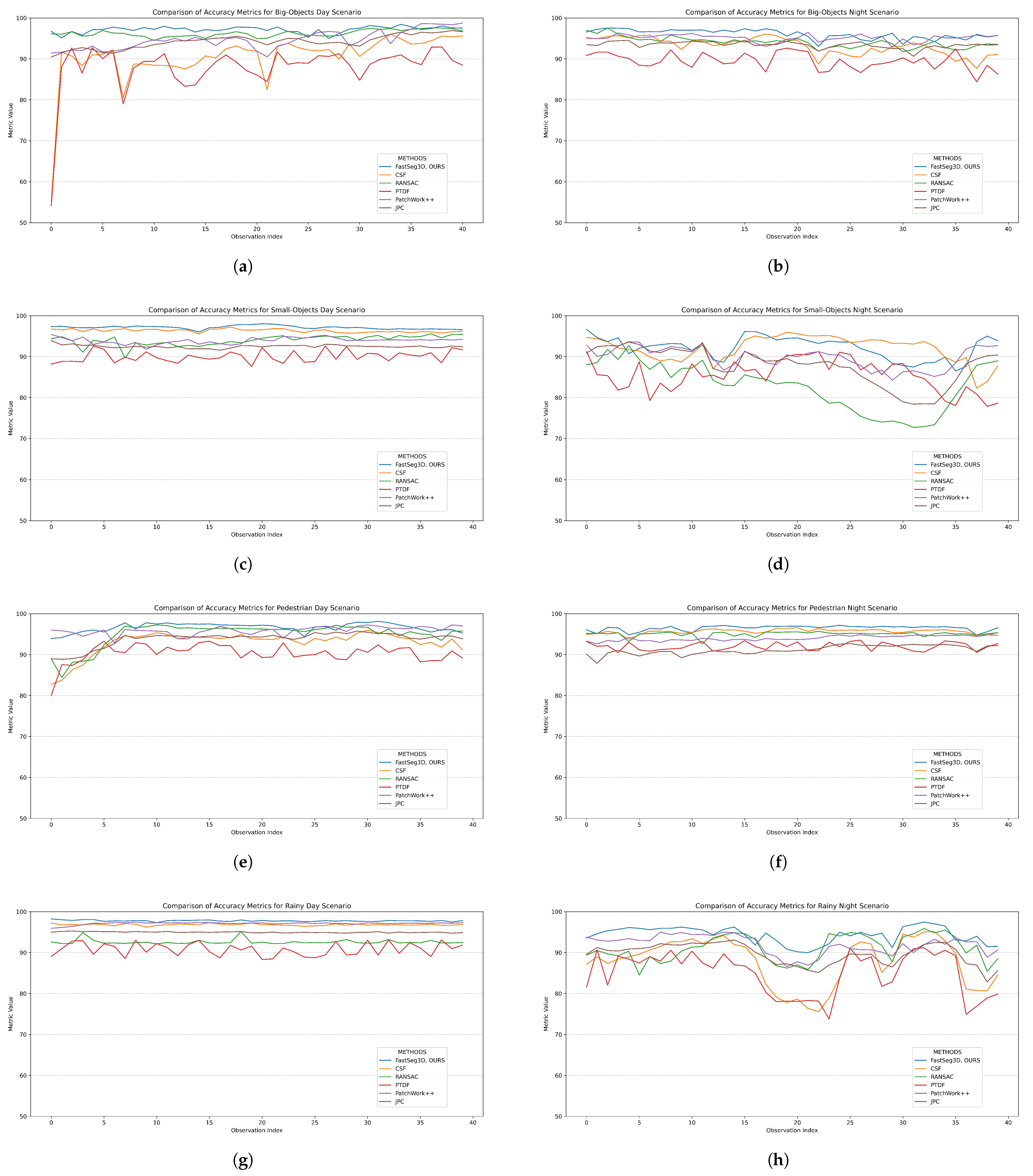
The kappa coefficient revealed how reliable all models compared were in the rainy and small-object night conditions. Overall the performance of the proposed algorithm was the most consistent across all test conditions. The mean kappa score was consistently above 90% except for the rainy and small-object scenarios in night test conditions. Figure 6 shows the accuracy graph of all methods across all samples, scenarios, and test conditions. Figure 6d,h also show how all methods struggled in performance for the rainy and small-object scenarios; however, the proposed algorithm performed consistently better.
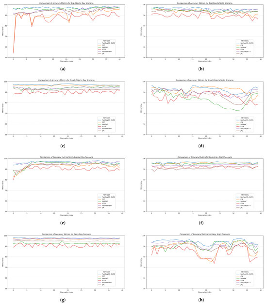
Figure 6.
Accuracy plot comparison of all methods (CSF [43], RANSAC [19], PTDF [23], Patchwork++ [75], and JPC [76]) across all scenarios. (a,b) Big-object, and dense-traffic day and night scenarios, respectively; (c,d) small-object and dense-traffic day and night scenarios, respectively; (e,f) pedestrian and dense-traffic day and night scenarios, respectively; (g,h) rainy scenes with busy traffic during the day and at night, respectively.
5. Conclusions
This study introduced FASTSeg3D, a fast and efficient ground segmentation algorithm designed for the real-time processing of 3D point clouds. The proposed method employed a two-stage approach, utilizing the range elevation estimation (REE) technique for fast organization and initial segmentation of point clouds, followed by a window-based model fitting (WBMF) technique to address over-segmentation and improve accuracy, using the unique geometric features of the initially segmented points. Through this combination, FASTSeg3D effectively handled complex terrains and reduced false positives while maintaining high computational efficiency.
Four common challenging scenarios were selected under two test conditions (day and night test conditions) to reflect the most common and most tasking scenarios in real-world navigation tasks. These scenarios included scenes with predominantly large objects such as vehicles in heavy or dense traffic, scenes with predominantly pedestrians in heavy or dense traffic, heavy and fast-moving traffic with lots of objects in rainy, cloudy weather, and scenes with predominantly small objects, like vegetation, debris, and traffic cones in heavy or dense traffic. A total of eight scenarios consisting of 313 samples were selected for testing and comparative analysis.
Results showed that FASTSEG3D was the most consistent of the compared methods in terms of segmentation accuracy, kappa coefficient, processing speed, intersection over union (IoU), error sensitivity, and F1 score. FASTSEG3D consistently achieved an error sensitivity rate of less than 10% across all scenarios, and its mean error remained below 7% for both ground and non-ground points in day and night test conditions. The algorithm maintained IoU scores above 90% across most test conditions, except in the challenging rainy and small-object night scenarios, where it still performed better than other methods.
Notably, FASTSEG3D’s F1 score remained above 90% across all scenarios, making it the only algorithm to achieve such performance consistency. The kappa coefficient demonstrated FASTSEG3D’s reliability, consistently maintaining a score above 90% across most conditions, again except for the most challenging rainy and small-object night scenarios. In terms of processing speed, FASTSEG3D outperformed other effective methods significantly, achieving a speed of approximately 10 times faster than that of the method with the most similar level of performance.
Future work will focus on three directions: (1) integrating intensity and temporal features to suppress rain-induced noise, inspired by recent advances in multi-modal filtering; (2) developing adaptive window sizing and thresholding to handle non-uniform terrains without manual tuning; and (3) deploying FASTSeg3D on embedded platforms (e.g., NVIDIA Jetson) to validate real-world applicability in autonomous vehicles. These enhancements aim to bridge the gap between controlled benchmarking and operational reliability in unstructured environments.
6. Patents
This manuscript is currently under patent consideration and is protected under a successfully filled provisional patent, which can be found at https://patentscope.wipo.int/search/en/WO2025052319 (accessed on 13 March 2025).
Author Contributions
Conceptualization, D.A.O.; methodology, D.A.O.; software, D.A.O.; validation, D.A.O.; formal analysis, D.A.O.; investigation, D.A.O.; resources, D.A.O. and E.D.M.; data curation, D.A.O.; writing—original draft preparation, D.A.O.; writing—review and editing, D.A.O.; visualization, D.A.O.; supervision, E.D.M. and A.M.A.-M.; project administration, E.D.M.; funding acquisition, E.D.M. and A.M.A.-M. All authors have read and agreed to the published version of the manuscript.
Funding
This research was supported by the Research and Development Centre at the Central University of Technology, Free State.
Institutional Review Board Statement
Not applicable.
Informed Consent Statement
Not applicable.
Data Availability Statement
The code is temporarily withheld pending patent approval but will be released upon publication. A demo version is accessible at. The nuScenes dataset is available at https://www.nuscenes.org/nuscenes (accessed on 25 April 2022).
Conflicts of Interest
The authors declare no conflicts of interest.
Abbreviations
The following abbreviations are used in this manuscript:
| REE | Range elevation estimation |
| WBMF | Window-based model fitting |
| PCA | Principal component analysis |
| SLAM | Simultaneous localization and mapping |
| 3D | Three-dimensional |
| LiDAR | Light Detection and Ranging |
| MLS | Mobile laser scanner |
| DTM | Digital Terrain Model |
| DSM | Digital Surface Model |
| RANSAC | Random sample consensus |
| GPR | Gaussian process regression |
| RLWR | Robust locally weighted regression |
| MCC | Multi-scale curvature classification |
| TPS | Thin-plate spline |
| TIN | Triangulated irregular network |
| PTDF | Progressive TIN Densification Filtering |
| CSF | Cloth Simulation Filtering |
| CRF | Conditional Random Field |
| MRF | Markov Random Field |
| PCD | Point cloud data |
| PMF | Progressive morphological filters |
| SMRF | Simple morphological filter |
| DMPs | Differential morphological profiles |
| bobj | Big-object and dense-traffic scenarios |
| sobj | Small-object and dense-traffic scenarios |
| ped | Pedestrian and dense-traffic scenarios |
| rainy | Rainy scenes with busy traffic |
Appendix A
Appendix A.1. Algorithm 1: REE
The complexity of the REE algorithm is the combined complexity needed to generate the 2D image and to determine the elevation of each point in the point cloud [83]. This can be expressed as follows:
where the size of the elevation structure is a maximum of N, which is the number of points in the point cloud, the maximum range is the same as the 2D range image height, h and represents the width and height of the 2D range image.
Appendix A.2. Algorithm 2: WBMF
The subset window column and window row, , was set to a dimension of , where is the range image width and is the range image height. This fixed dimension satisfied the condition that w is less than or equal to r and r divides w without a remainder. The same applied to c and a. Therefore,
Using the initial ground points as candidate points, i.e., , in a sliding-window manner, as shown in Figure 4, the best seed points were determined from initial ground points in the current window. This was selected based on the first k set number of initial ground points with the lowest elevation value in the current window, which is indicated by superscript i, where k was a minimum of 5 and a maximum of 20 points in the current window, i. This was expressed as:
Using the best seed points for the current window, the covariance matrix M and the eigenvectors and eigenvalues of the covariance matrix M were calculated. M, eigenvectors, and eigenvalues were calculated using the standard covariance matrix formula for the principal component analysis (PCA) [74]. A plane model was computed. This model was developed using the normal vector to the plane equation. The normal vector of the plane model was . This can be expressed as:
The normal vector of the plane model was used to compute unique features, adaptively, for all points in the current window. These features included the distance for points from the normal vector , the elevation of the point reference to the normal vector , and the angle of inclination of the point reference to the normal vector. is the distance for points in the current window to the plane origin or normal vector distance d. The normal vector distance d, as expressed in Equation (A5), is the point of origin for the current window. The new values were updated to the data structure of the point cloud; therefore, the coordinates would match the coordinate of the data structure. These values were expressed as:
A set threshold was used to filter out non-ground points from initially segmented ground points. The WBMF thresholds () were determined via grid search on a 20% validation subset of nuScenes, optimizing the F1 score while ensuring real-time performance. These values aligned with prior works [84,85,86]:
- : ground points within of the plane model minimized false positives [84,85].
- : slopes rarely corresponded to drivable surfaces in urban settings [84].
- matched REE’s tolerance to ensure consistency [84,86].
The complexity of the WBMF algorithm is the combined complexity needed for the fraction of window to successfully slide over the entire image and requires the surface normal for each window [83]. This can be expressed as:
where N is the number of points in the point cloud, W is the temporal storage of points for a given window, n is the number of points temporarily stored and used to calculate the surface normal for a given window, which is a constant with a minimum of 5 and a maximum of 20. are the fractions of rows and columns for a given window, W is the total number of windows or slides over the 2D range image, which is constant, and P is the total number of cells in the 2D image, which is .
References
- Pendleton, S.; Andersen, H.; Du, X.; Shen, X.; Meghjani, M.; Eng, Y.; Rus, D.; Ang, M. Perception, Planning, Control, and Coordination for Autonomous Vehicles. Machines 2017, 5, 6. [Google Scholar] [CrossRef]
- Roy, A.; Todorovic, S. Monocular Depth Estimation Using Neural Regression Forest. In Proceedings of the IEEE Conference on Computer Vision and Pattern Recognition (CVPR), Las Vegas, NV, USA, 27–30 June 2016; pp. 5506–5514. [Google Scholar]
- Saxena, A.; Schulte, J.; Ng, A. Depth Estimation using Monocular and Stereo Cues. In IJCAI’07, Proceedings of the 20th International Joint Conference on Artificial Intelligence, Nagoya, Japan, 6–12 January 2007; Morgan Kaufmann Publishers Inc.: San Francisco, CA, USA, 2007; pp. 2197–2203. [Google Scholar]
- Qin, R.; Tian, J.; Reinartz, P. 3D change detection—Approaches and applications. ISPRS J. Photogramm. Remote Sens. 2016, 122, 41–56. [Google Scholar] [CrossRef]
- Shan, J. Topographic Laser Ranging and Scanning, 2nd ed.; CRC Press: Boca Raton, FL, USA, 2018. [Google Scholar]
- Meng, X.; Currit, N.; Zhao, K. Ground Filtering Algorithms for Airborne LiDAR Data: A Review of Critical Issues. Remote Sens. 2010, 2, 833–860. [Google Scholar] [CrossRef]
- Nguyen, A.; Le, B. 3D point cloud segmentation: A survey. In Proceedings of the 2013 6th IEEE Conference on Robotics, Automation and Mechatronics (RAM), Manila, Phillippines, 12–15 November 2013; pp. 225–230. [Google Scholar] [CrossRef]
- Xie, Y.; Tian, J.; Zhu, X. Linking Points With Labels in 3D: A Review of Point Cloud Semantic Segmentation. IEEE Geosci. Remote Sens. Mag. 2019, 8, 38–59. [Google Scholar] [CrossRef]
- Jozdani, S.; Chen, D.; Pouliot, D.; Alan Johnson, B. A review and meta-analysis of Generative Adversarial Networks and their applications in remote sensing. Int. J. Appl. Earth Obs. Geoinf. 2022, 108, 102734. [Google Scholar] [CrossRef]
- Lim, J.; Santinelli, G.; Dahal, A.; Vrieling, A.; Lombardo, L. An ensemble neural network approach for space–time landslide predictive modelling. Int. J. Appl. Earth Obs. Geoinf. 2024, 132, 104037. [Google Scholar] [CrossRef]
- Qin, N.; Tan, W.; Guan, H.; Wang, L.; Ma, L.; Tao, P.; Fatholahi, S.; Hu, X.; Li, J. Towards intelligent ground filtering of large-scale topographic point clouds: A comprehensive survey. Int. J. Appl. Earth Obs. Geoinf. 2023, 125, 103566. [Google Scholar] [CrossRef]
- Garnelo, M.; Shanahan, M. Reconciling deep learning with symbolic artificial intelligence: Representing objects and relations. Curr. Opin. Behav. Sci. 2019, 29, 17–23. [Google Scholar] [CrossRef]
- Poux, F.; Billen, R. Voxel-based 3D Point Cloud Semantic Segmentation: Unsupervised Geometric and Relationship Featuring vs Deep Learning Methods. ISPRS Int. J. Geo-Inf. 2019, 8, 213. [Google Scholar] [CrossRef]
- Poux, F.d.L.U.; Mattes, C.; Kobbelt, L. Unsupervised segmentation of indoor 3D point cloud: Application to object-based classification. Int. Arch. Photogramm. Remote Sens. Spat. Inf. Sci. 2020, 44, 111–118. [Google Scholar] [CrossRef]
- Xue, F.; Lu, W.; Chen, Z.; Webster, C. From LiDAR point cloud towards digital twin city: Clustering city objects based on Gestalt principles. ISPRS J. Photogramm. Remote Sens. 2020, 167, 418–431. [Google Scholar] [CrossRef]
- Chen, Z.; Deng, L.; Luo, Y.; Li, D.; Marcato Junior, J.; Nunes Gonçalves, W.; Awal Md Nurunnabi, A.; Li, J.; Wang, C.; Li, D. Road extraction in remote sensing data: A survey. Int. J. Appl. Earth Obs. Geoinf. 2022, 112, 102833. [Google Scholar] [CrossRef]
- Xiao, W.; Cao, H.; Tang, M.; Zhang, Z.; Chen, N. 3D urban object change detection from aerial and terrestrial point clouds: A review. Int. J. Appl. Earth Obs. Geoinf. 2023, 118, 103258. [Google Scholar] [CrossRef]
- Chen, T.; Dai, B.; Liu, D.; Song, J. Sparse Gaussian process regression based ground segmentation for autonomous land vehicles. In Proceedings of the 27th Chinese Control and Decision Conference (2015 CCDC), Qingdao, China, 23–25 May 2015; pp. 3993–3998. [Google Scholar] [CrossRef]
- Fischler, M.; Bolles, R. Random sample consensus. Commun. ACM 1981, 24, 381–395. [Google Scholar] [CrossRef]
- Kraus, K.; Pfeifer, N. Determination of terrain models in wooded areas with airborne laser scanner data. ISPRS J. Photogramm. Remote Sens. 1998, 53, 193–203. [Google Scholar] [CrossRef]
- Kraus, K.; Pfeifer, N. Advanced DTM generation from LIDAR data. Int. Arch. Photogramm. Remote Sens. Spat. Inf. Sci. 2001, 34, 23–30. [Google Scholar]
- Pfeifer, N.; Reiter, T.; Briese, C.; Rieger, W. Interpolation of high quality ground models from laser scanner data in forested areas. Int. Arch. Photogramm. Remote Sens. 1999, 32, 31–36. [Google Scholar]
- Axelsson, P. DEM generation from laser scanner data using adaptive TIN models. Int. Arch. Photogramm. Remote Sens. 2000, 33, 110–117. [Google Scholar]
- Zhao, X.; Guo, Q.; Su, Y.; Xue, B. Improved progressive TIN densification filtering algorithm for airborne LiDAR data in forested areas. ISPRS J. Photogramm. Remote Sens. 2016, 117, 79–91. [Google Scholar] [CrossRef]
- Dai, W.; Kan, H.; Tan, R.; Yang, B.; Guan, Q.; Zhu, N.; Xiao, W.; Dong, Z. Multisource forest point cloud registration with semantic-guided keypoints and robust RANSAC mechanisms. Int. J. Appl. Earth Obs. Geoinf. 2022, 115, 103105. [Google Scholar] [CrossRef]
- Diaz, N.; Gallo, O.; Caceres, J.; Porras, H. Real-time ground filtering algorithm of cloud points acquired using Terrestrial Laser Scanner (TLS). Int. J. Appl. Earth Obs. Geoinf. 2021, 105, 102629. [Google Scholar] [CrossRef]
- Ji, X.; Yang, B.; Tang, Q.; Xu, W.; Li, J. Feature fusion-based registration of satellite images to airborne LiDAR bathymetry in island area. Int. J. Appl. Earth Obs. Geoinf. 2022, 109, 102778. [Google Scholar] [CrossRef]
- Chen, T.; Dai, B.; Wang, R.; Liu, D. Gaussian-Process-Based Real-Time Ground Segmentation for Autonomous Land Vehicles. J. Intell. Robot. Syst. 2013, 76, 563–582. [Google Scholar] [CrossRef]
- Liu, K.; Wang, W.; Tharmarasa, R.; Wang, J.; Zuo, Y. Ground surface filtering of 3D point clouds based on hybrid regression technique. IEEE Access 2019, 7, 23270–23284. [Google Scholar] [CrossRef]
- Zermas, D.; Izzat, I.; Papanikolopoulos, N. Fast segmentation of 3D point clouds: A paradigm on LiDAR data for autonomous vehicle applications. In Proceedings of the 2017 IEEE International Conference on Robotics and Automation (ICRA), Singapore, 29 May–3 June 2017; pp. 5067–5073. [Google Scholar] [CrossRef]
- Briese, C.; Pfeifer, N.; Stadler, P. Derivation of Digital Terrain Models in the SCOP++ Environment. In Proceedings of the OEEPE Workshop on Airborne Laserscanning and Interferometric SAR for Digital Elevation Models, Stockholm, Sweden, 1–3 March 2001; p. 13. [Google Scholar]
- Evans, J.; Hudak, A. A multiscale curvature algorithm for classifying discrete return LiDAR in forested environments. IEEE Trans. Geosci. Remote Sens. 2007, 45, 1029–1038. [Google Scholar] [CrossRef]
- Mongus, D.; Žalik, B. Parameter-free ground filtering of LiDAR data for automatic DTM generation. ISPRS J. Photogramm. Remote Sens. 2012, 67, 1–12. [Google Scholar] [CrossRef]
- Hu, H.; Ding, Y.; Zhu, Q.; Wu, B.; Lin, H.; Du, Z.; Zhang, Y.; Zhang, Y. An adaptive surface filter for airborne laser scanning point clouds by means of regularization and bending energy. ISPRS J. Photogramm. Remote Sens. 2014, 92, 98–111. [Google Scholar] [CrossRef]
- Liu, X.; Zhang, Y.; Huang, X.; Wan, Y.; Zhang, Y.; Wang, S. Terrain-Adaptive Ground Filtering of Airborne LiDAR Data Based on Saliency-Aware Thin Plate Spline. Int. Arch. Photogramm. Remote Sens. Spat. Inf. Sci. 2020, XLIII-B2-2, 279–285. [Google Scholar] [CrossRef]
- Qin, L.; Wu, W.; Tian, Y.; Xu, W. LiDAR Filtering of Urban Areas with Region Growing Based on Moving-Window Weighted Iterative Least-Squares Fitting. IEEE Geosci. Remote Sens. Lett. 2017, 14, 841–845. [Google Scholar] [CrossRef]
- Adams, R.; Bischof, L. Seeded Region Growing. IEEE Trans. Pattern Anal. Mach. Intell. 1994, 16, 641–647. [Google Scholar] [CrossRef]
- Hojjatoleslami, S.; Kittler, J. Region growing: A new approach. IEEE Trans. Image Process. 1998, 7, 1079–1084. [Google Scholar] [CrossRef] [PubMed]
- Chen, Q.; Wang, H.; Zhang, H.; Sun, M.; Liu, X. A Point Cloud Filtering Approach to Generating DTMs for Steep Mountainous Areas and Adjacent Residential Areas. Remote Sens. 2016, 8, 71. [Google Scholar] [CrossRef]
- Dong, Y.; Cui, X.; Zhang, L.; Ai, H. An improved progressive TIN densification filtering method considering the density and standard variance of point clouds. ISPRS Int. J. Geo-Inf. 2018, 7, 409. [Google Scholar] [CrossRef]
- Zhang, J.; Lin, X. Filtering airborne LiDAR data by embedding smoothness-constrained segmentation in progressive TIN densification. ISPRS J. Photogramm. Remote Sens. 2013, 81, 44–59. [Google Scholar] [CrossRef]
- Elmqvist, M. Ground surface estimation from airborne laser scanner data using active shape models 1.1. Int. Arch. Photogramm. Remote Sens. (ISPRS) 2002, 34, 114–118. [Google Scholar]
- Zhang, W.; Qi, J.; Wan, P.; Wang, H.; Xie, D.; Wang, X.; Yan, G. An Easy-to-Use Airborne LiDAR Data Filtering Method Based on Cloth Simulation. Remote Sens. 2016, 8, 501. [Google Scholar] [CrossRef]
- Dakin Kuiper, S.; Coops, N.; Jarron, L.; Tompalski, P.; White, J. An automated approach to detecting instream wood using airborne laser scanning in small coastal streams. Int. J. Appl. Earth Obs. Geoinf. 2023, 118, 103272. [Google Scholar] [CrossRef]
- Hillman, S.; Wallace, L.; Lucieer, A.; Reinke, K.; Turner, D.; Jones, S. A comparison of terrestrial and UAS sensors for measuring fuel hazard in a dry sclerophyll forest. Int. J. Appl. Earth Obs. Geoinf. 2021, 95, 102261. [Google Scholar] [CrossRef]
- Yu, D.; He, L.; Ye, F.; Jiang, L.; Zhang, C.; Fang, Z.; Liang, Z. Unsupervised ground filtering of airborne-based 3D meshes using a robust cloth simulation. Int. J. Appl. Earth Obs. Geoinf. 2022, 111, 102830. [Google Scholar] [CrossRef]
- Vosselman, G. Slope Based Filtering of Laser Altimetry Data. Int. Arch. Photogramm. Remote Sens. 2000, 33, 935–942. [Google Scholar]
- Meng, X.; Wang, L.; Silván-Cárdenas, J.; Currit, N. A multi-directional ground filtering algorithm for airborne LIDAR. ISPRS J. Photogramm. Remote Sens. 2009, 64, 117–124. [Google Scholar] [CrossRef]
- Susaki, J. Adaptive Slope Filtering of Airborne LiDAR Data in Urban Areas for Digital Terrain Model (DTM) Generation. Remote Sens. 2012, 4, 1804–1819. [Google Scholar] [CrossRef]
- Wang, C.K.; Tseng, Y.H. Dual-directional profile filter for digital terrain model generation from airborne laser scanning data. J. Remote Sens. 2014, 8, 083619. [Google Scholar] [CrossRef]
- Thrun, S.; Montemerlo, M.; Dahlkamp, H.; Stavens, D.; Aron, A.; Diebel, J.; Fong, P.; Gale, J.; Halpenny, M.; Hoffmann, G.; et al. Stanley: The Robot that Won the DARPA Grand Challenge. J. Field Robot. 2006, 23, 661–692. [Google Scholar] [CrossRef]
- Goga, S.; Nedevschi, S. An approach for segmenting 3D LiDAR data using multi-volume grid structures. In Proceedings of the 2017 13th IEEE International Conference on Intelligent Computer Communication and Processing (ICCP), Cluj-Napoca, Romania, 7–9 September 2017; pp. 309–315. [Google Scholar] [CrossRef]
- Moosmann, F.; Pink, O.; Stiller, C. Segmentation of 3D lidar data in non-flat urban environments using a local convexity criterion. In Proceedings of the 2009 IEEE Intelligent Vehicles Symposium, Xi’an, China, 3–5 June 2009; pp. 215–220. [Google Scholar] [CrossRef]
- Yang, B.; Dong, Z. A shape-based segmentation method for mobile laser scanning point clouds. ISPRS J. Photogramm. Remote Sens. 2013, 81, 19–30. [Google Scholar] [CrossRef]
- Rummelhard, L.; Paigwar, A.; Negre, A.; Laugier, C. Ground estimation and point cloud segmentation using SpatioTemporal Conditional Random Field. In Proceedings of the 2017 IEEE Intelligent Vehicles Symposium (IV), Los Angeles, CA, USA, 11–14 June 2017; pp. 1105–1110. [Google Scholar] [CrossRef]
- Zhang, M.; Morris, D.; Fu, R. Ground Segmentation Based on Loopy Belief Propagation for Sparse 3D Point Clouds. In Proceedings of the 2015 IEEE International Conference on 3D Vision (3DV), Lyon, France, 19–22 October 2015; pp. 615–622. [Google Scholar] [CrossRef]
- Haralick, R.; Sternberg, S.; Zhuang, X. Image Analysis Using Mathematical Morphology. IEEE Trans. Pattern Anal. Mach. Intell. 1987, 9, 532–550. [Google Scholar] [CrossRef] [PubMed]
- Schafer, R. Morphological filters—Part I: Their set-theoretic analysis and relations to linear shift-invariant filters. IEEE Trans. Acoust. 1987, 35, 1153–1169. [Google Scholar] [CrossRef]
- Soille, P. Morphological Operators; Academic Press: Cambridge, MA, USA, 2000; pp. 483–515. [Google Scholar] [CrossRef]
- Kilian, J.; Haala, N.; Englich, M. Capture and evaluation of airborne laser scanner data. In Proceedings of the International Archives of the Photogrammetry, Remote Sensing and Spatial Information Sciences, Vienna, Austria, 9–19 July 1996; Volume 31, pp. 383–388. [Google Scholar]
- Zhang, K.; Chen, S.; Whitman, D.; Shyu, M.; Yan, J.; Zhang, C. A progressive morphological filter for removing nonground measurements from airborne LIDAR data. IEEE Trans. Geosci. Remote Sens. 2003, 41, 872–882. [Google Scholar] [CrossRef]
- Chen, Q.; Gong, P.; Baldocchi, D.; Xie, G. Filtering Airborne Laser Scanning Data with Morphological Methods. Photogramm. Eng. Remote Sens. 2007, 73, 175–185. [Google Scholar] [CrossRef]
- Pingel, T.; Clarke, K.; McBride, W. An improved simple morphological filter for the terrain classification of airborne LIDAR data. ISPRS J. Photogramm. Remote Sens. 2013, 77, 21–30. [Google Scholar] [CrossRef]
- Mongus, D.; Lukač, N.; Žalik, B. Ground and building extraction from LiDAR data based on differential morphological profiles and locally fitted surfaces. ISPRS J. Photogramm. Remote Sens. 2014, 93, 145–156. [Google Scholar] [CrossRef]
- Hao, Y.; Zhen, Z.; Li, F.; Zhao, Y. A graph-based progressive morphological filtering (GPMF) method for generating canopy height models using ALS data. Int. J. Appl. Earth Obs. Geoinf. 2019, 79, 84–96. [Google Scholar] [CrossRef]
- Li, Y.; Yong, B.; van Oosterom, P.; Lemmens, M.; Wu, H.; Ren, L.; Zheng, M.; Zhou, J. Airborne LiDAR Data Filtering Based on Geodesic Transformations of Mathematical Morphology. Remote Sens. 2017, 9, 1104. [Google Scholar] [CrossRef]
- Liu, L.; Lim, S. A voxel-based multiscale morphological airborne lidar filtering algorithm for digital elevation models for forest regions. Measurement 2018, 123, 135–144. [Google Scholar] [CrossRef]
- Schindler, J.; Dymond, J.; Wiser, S.; Shepherd, J. Method for national mapping spatial extent of southern beech forest using temporal spectral signatures. Int. J. Appl. Earth Obs. Geoinf. 2021, 102, 102408. [Google Scholar] [CrossRef]
- Fong, W.; Mohan, R.; Hurtado, J.; Zhou, L.; Caesar, H.; Beijbom, O.; Valada, A. Panoptic nuScenes: A Large-Scale Benchmark for LiDAR Panoptic Segmentation and Tracking. IEEE Robot. Autom. Lett. 2021, 7, 3795–3802. [Google Scholar] [CrossRef]
- Cheng, Y.; Patel, A.; Wen, C.; Bullock, D.; Habib, A. Intensity Thresholding and Deep Learning Based Lane Marking Extraction and Lane Width Estimation from Mobile Light Detection and Ranging (LiDAR) Point Clouds. Remote Sens. 2020, 12, 1379. [Google Scholar] [CrossRef]
- Zhao, X.; Yang, Z.; Schwertfeger, S. Mapping with Reflection—Detection and Utilization of Reflection in 3D Lidar Scans. In Proceedings of the 2020 IEEE International Symposium on Safety, Security, and Rescue Robotics, Abudhabi, United Arab Emirates, 4–6 November 2020; pp. 27–33. [Google Scholar] [CrossRef]
- Kukko, A.; Kaasalainen, S.; Litkey, P. Effect of incidence angle on laser scanner intensity and surface data. Appl. Opt. 2008, 47, 986–992. [Google Scholar] [CrossRef]
- Huang, W.; Liang, H.; Lin, L.; Wang, Z.; Wang, S.; Yu, B.; Niu, R. A Fast Point Cloud Ground Segmentation Approach Based on Coarse-To-Fine Markov Random Field. IEEE Trans. Intell. Transp. Syst. 2022, 23, 7841–7854. [Google Scholar] [CrossRef]
- Maćkiewicz, A.; Ratajczak, W. Principal components analysis (PCA). Comput. Geosci. 1993, 19, 303–342. [Google Scholar] [CrossRef]
- Lee, S.; Lim, H.; Myung, H. Patchwork++: Fast and Robust Ground Segmentation Solving Partial Under-Segmentation Using 3D Point Cloud. In Proceedings of the 2022 IEEE/RSJ International Conference on Intelligent Robots and Systems (IROS), Kyoto, Japan, 23–27 October 2022; pp. 13276–13283. [Google Scholar] [CrossRef]
- Shen, Z.; Liang, H.; Lin, L.; Wang, Z.; Huang, W.; Yu, J. Fast Ground Segmentation for 3D LiDAR Point Cloud Based on Jump-Convolution-Process. Remote Sens. 2021, 13, 3239. [Google Scholar] [CrossRef]
- Caesar, H.; Bankiti, V.; Lang, A.; Vora, S.; Liong, V.; Xu, Q.; Krishnan, A.; Pan, Y.; Baldan, G.; Beijbom, O. nuScenes: A multimodal dataset for autonomous driving. In Proceedings of the IEEE/CVF Conference on Computer Vision and Pattern Recognition, Seattle, WA, USA, 13–19 June 2020; pp. 11618–11628. [Google Scholar] [CrossRef]
- Cohen, J. Weighted kappa: Nominal scale agreement provision for scaled disagreement or partial credit. Psychol. Bull. 1968, 70, 213–220. [Google Scholar] [CrossRef] [PubMed]
- Rezatofighi, H.; Tsoi, N.; Gwak, J.; Sadeghian, A.; Reid, I.; Savarese, S. Generalized Intersection Over Union: A Metric and a Loss for Bounding Box Regression. In Proceedings of the IEEE/CVF Conference on Computer Vision and Pattern Recognition, Long Beach, CA, USA, 15–20 June 2019; pp. 658–666. [Google Scholar]
- Sokolova, M.; Japkowicz, N.; Szpakowicz, S. Beyond Accuracy, F-Score and ROC: A Family of Discriminant Measures for Performance Evaluation. In Proceedings of the AI 2006: Advances in Artificial Intelligence; Sattar, A., Kang, B.H., Eds.; Springer: Berlin/Heidelberg, Germany, 2006; pp. 1015–1021. [Google Scholar]
- Rusu, R.; Cousins, S. 3D is here: Point Cloud Library (PCL). In Proceedings of the IEEE International Conference on Robotics and Automation (ICRA), Shanghai, China, 9–13 May 2011. [Google Scholar]
- Geometron GmbH. Fade2.5D: C++ Delaunay Triangulation Library, 2D and 2.5D with Examples. Available online: https://www.geom.at/fade25d/html/ (accessed on 24 April 2024).
- Arora, S.; Barak, B. Computational Complexity: A Modern Approach; Cambridge University Press: Cambridge, UK, 2006. [Google Scholar]
- Bailey, G.; Li, Y.; McKinney, N.; Yoder, D.; Wright, W.; Herrero, H. Comparison of Ground Point Filtering Algorithms for High-Density Point Clouds Collected by Terrestrial LiDAR. Remote Sens. 2022, 14, 4776. [Google Scholar] [CrossRef]
- Zheng, Z.; Wang, C.; Liu, H.; Tan, Y. Adaptive random sample consensus method for ground filtering of airborne LiDAR. J. Phys. Conf. Ser. 2023, 2478, 102030. [Google Scholar] [CrossRef]
- Fan, W.; Liu, X.; Zhang, Y.; Yue, D.; Wang, S.; Zhong, J. Airborne LiDAR Point Cloud Filtering Algorithm Based on Supervoxel Ground Saliency. ISPRS Ann. Photogramm. Remote Sens. Spat. Inf. Sci. 2024, X, 73–79. [Google Scholar] [CrossRef]

Disclaimer/Publisher’s Note: The statements, opinions and data contained in all publications are solely those of the individual author(s) and contributor(s) and not of MDPI and/or the editor(s). MDPI and/or the editor(s) disclaim responsibility for any injury to people or property resulting from any ideas, methods, instructions or products referred to in the content. |
© 2025 by the authors. Licensee MDPI, Basel, Switzerland. This article is an open access article distributed under the terms and conditions of the Creative Commons Attribution (CC BY) license (https://creativecommons.org/licenses/by/4.0/).