
XNODE: A XAI Suite to Understand Neural Ordinary Differential Equations


Abstract
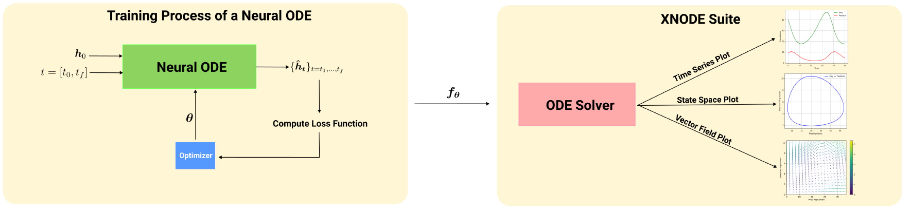
1. Introduction
- A numerical ODE solver that computes the approximate solution of (2).
- The neural network , which is evaluated at each time step within the solver.
2. Background on Systems of Differential Equations
Lyapunov Stability and Attractors, Repellers, and Saddle Points
- for all and all t,
- for all t,
- The total derivative satisfies
3. Explainability and Neural ODEs
3.1. The XNODE Suite
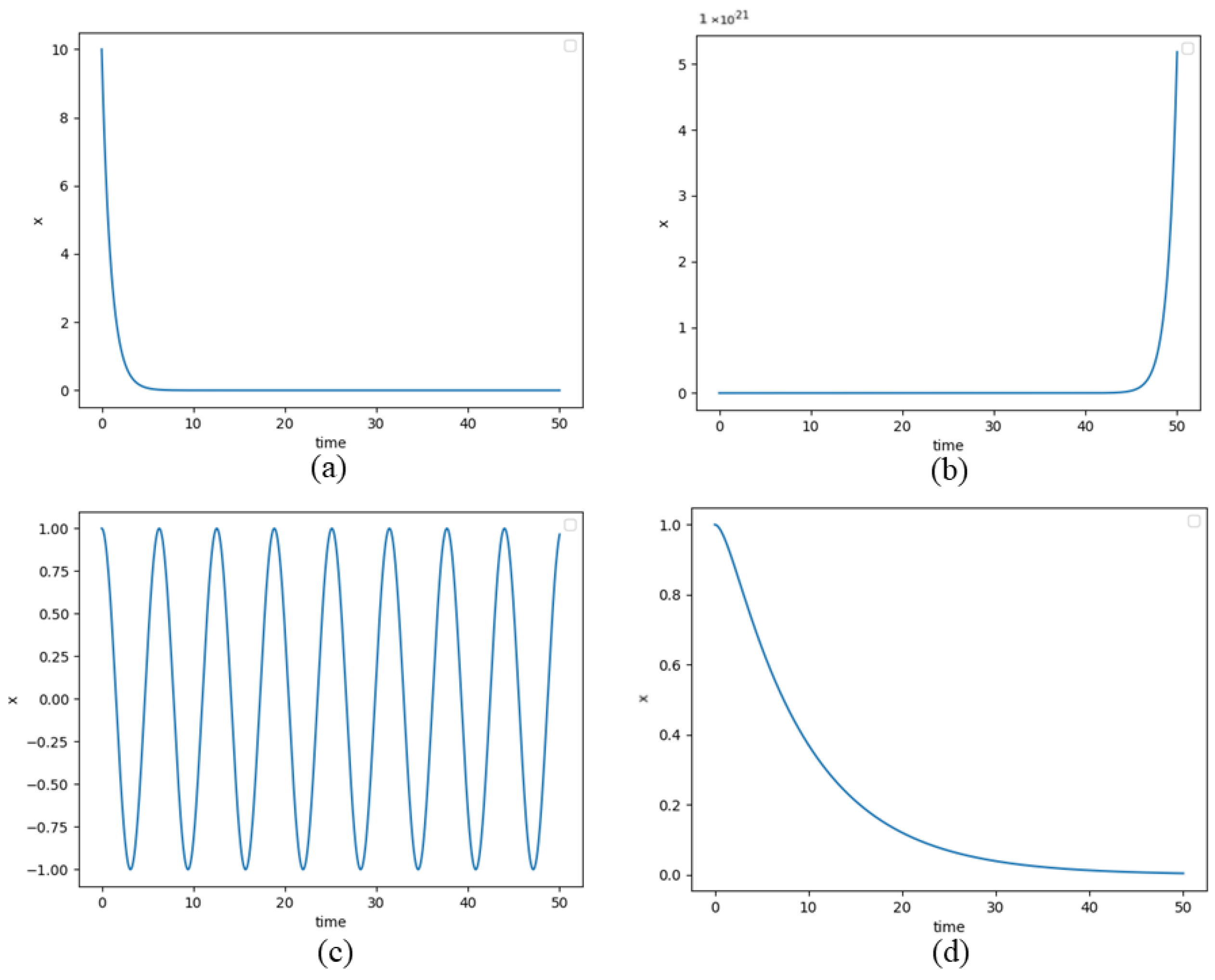
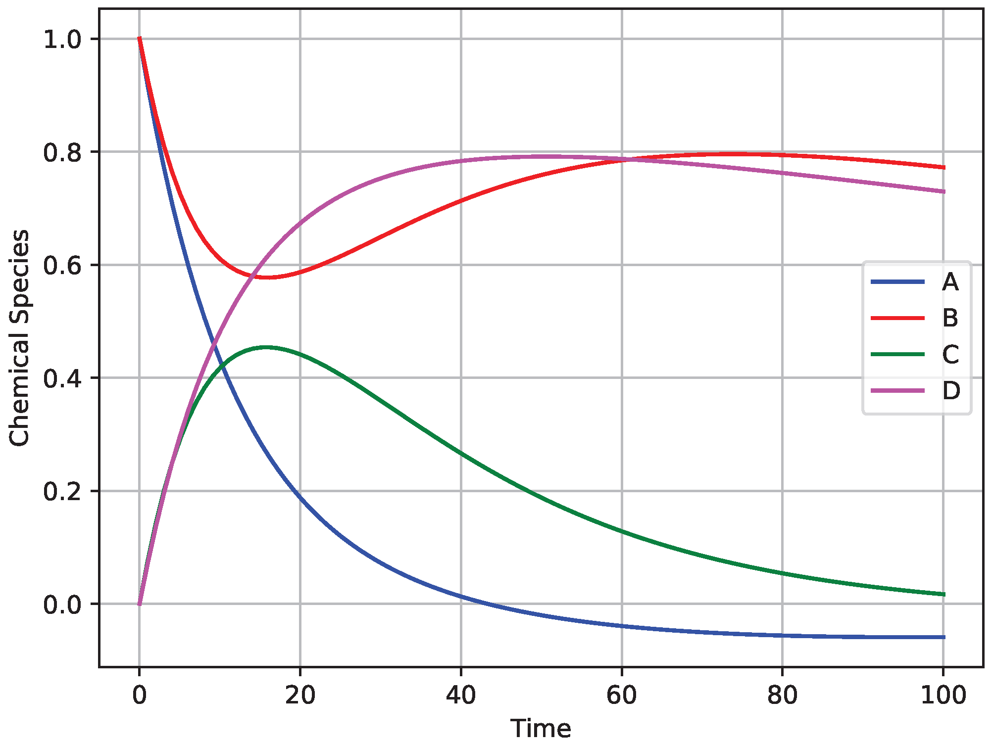
3.1.1. Time Series Plots
- Stability: This involves identifying stable and unstable regions within the solution space. Stable equilibria feature trajectories that converge towards fixed points, whereas unstable equilibria exhibit divergence. These plots help to detect critical points and bifurcations, making stability analysis more intuitive (Figure 2a,b).
- Periodicity: Repetitive patterns reveal the frequency, amplitude, and period of oscillations, aiding in the interpretation of rhythmic dynamics (Figure 2c).
- Transience: Transient behaviours capture a system’s evolution from the initial conditions to a steady state. These plots highlight relaxation to equilibrium and responses to perturbations, making transient phenomena more cleare (Figure 2d).
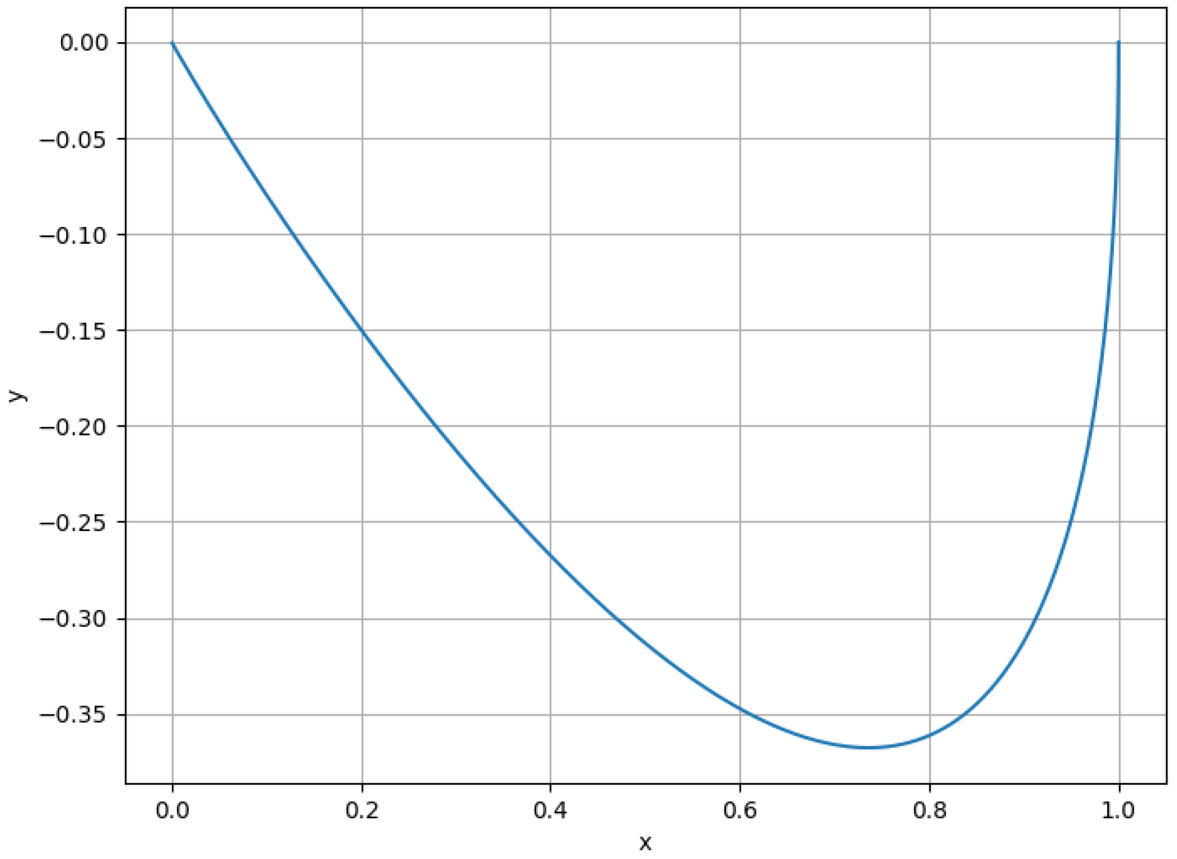
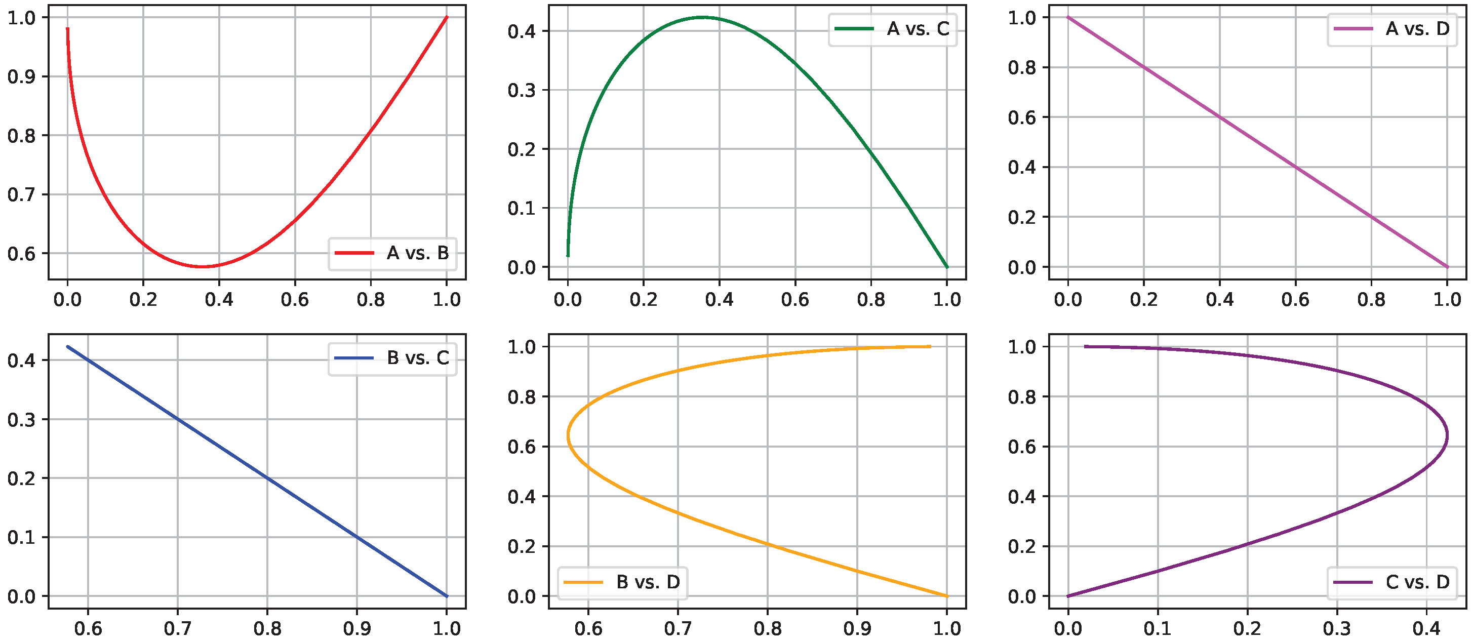
3.1.2. State Space Plots
- Variable Dynamics: This visualization helps to identify relationships and patterns, enhancing the explanation of the system’s behavior (Figure 3).
| Algorithm 1 Construction of state space plots. |
|
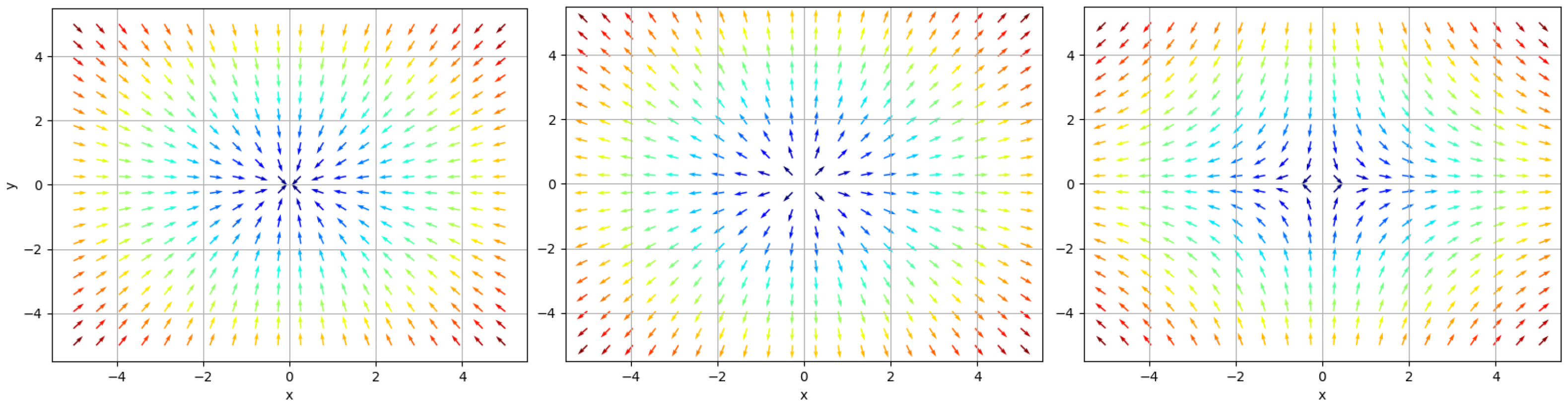
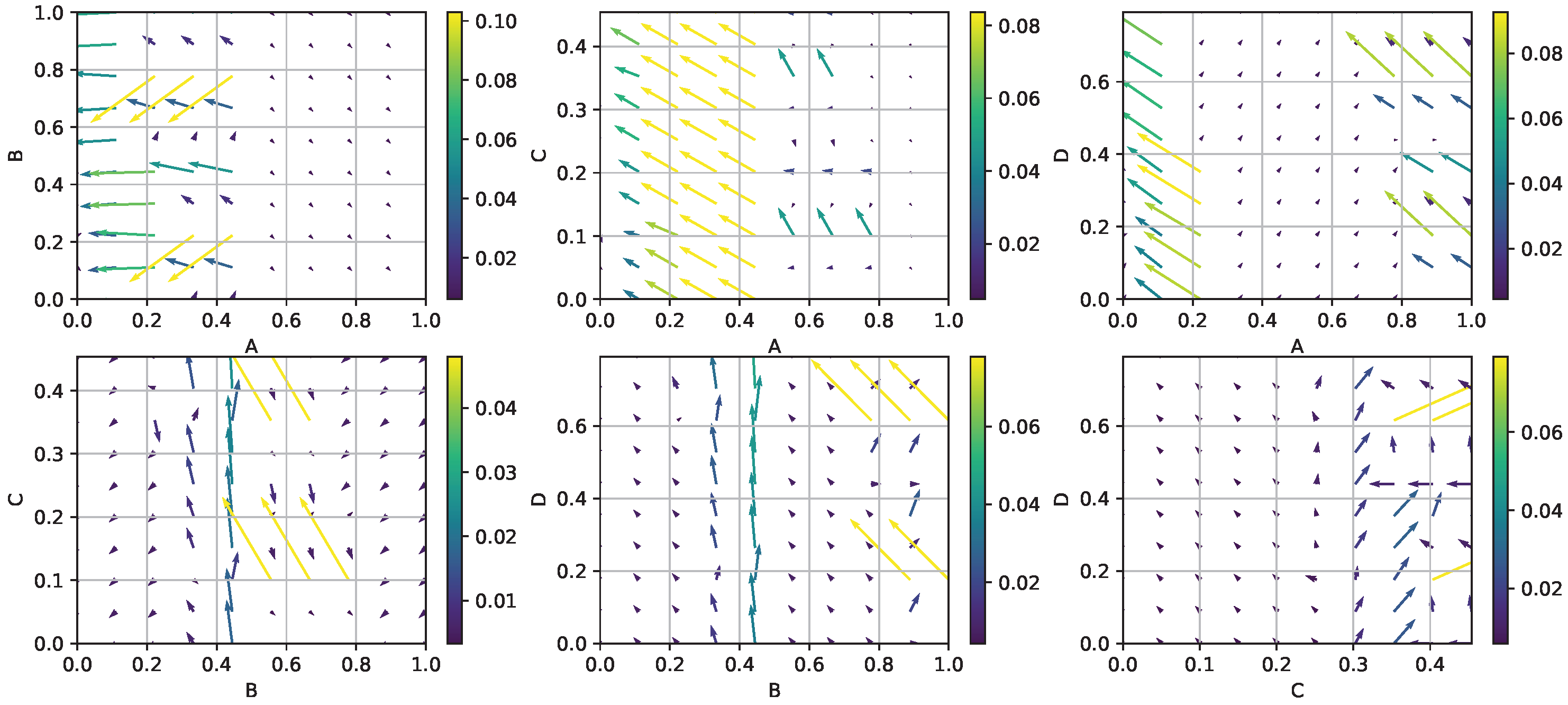
3.1.3. Vector Field Plots
| Algorithm 2 Construction of two-dimensional vector field plots. |
|
3.2. Beyond Improving Explainability
- Data Anomaly Detection. The XNODE suite techniques allow for the visualisation of the model dynamics through time, enabling detection of unusual or unexpected behaviours. Anomalies such as sudden deviations, irregular patterns, and unexpected behaviour when subjected to scrutiny by domain experts may serve as indicators warranting attention. Such occurrences may indicate possible poor data quality, which can emerge as anomalies, errors, or outliers. The identification of possible data anomalies is essential for ensuring the reliability of the resulting models.
- Debugging. In the process of modelling real-world systems based on data, large amounts of high-quality data are indispensable for Neural ODEs to effectively capture the intrinsic dynamics of a system and yield robust models. Unfortunately, the scarcity of such large amounts of high-quality data is a prevalent challenge that compromises the output quality of the generated models. In addition, the black-box nature of NNs makes the identification of such problems more difficult. This issue becomes particularly problematic when the systems under consideration are governed by well-defined physical principles that are known a priori; in such cases, the failure of NN models to successfully extract these governing rules from the available data results in non-meaningful predictions, causing field experts to distrust the use of NNs. The proposed XNODE suite techniques can mitigate this issue by providing field experts with insights into the level at which Neural ODE models satisfy physical constraints, i.e., their success (or lack thereof) in extracting the underlying rules from the data. These techniques assist in identifying potential problems by pointing out regions of instability or non-conformance to the expected dynamics. By offering a nuanced understanding of model performance, the XNODE suite can represent a valuable tool for mitigating the challenges posed by data scarcity and ensuring the reliability of the models in scenarios where adherence to known physical principles is crucial.
- Performance Optimisation. The visualisation of Neural ODE model dynamics is a valuable tool for enhancing model performance by providing insights into the optimisation of training hyperparameters. This visual examination enables field experts to determine necessary adjustments, especially concerning the choice of integration schemes employed within the Neural ODE solver. Through application of the XNODE suite techniques, field experts can systematically compare the dynamics produced by different integration schemes showing which scheme aligns more closely with the anticipated behaviour of the modelled systems.
4. Experiments
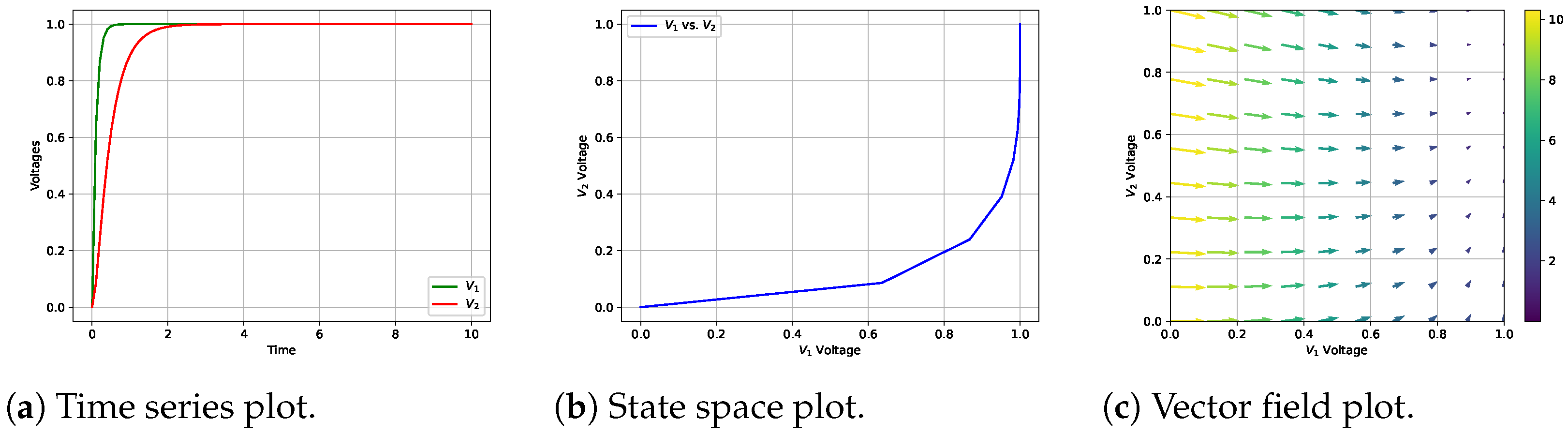
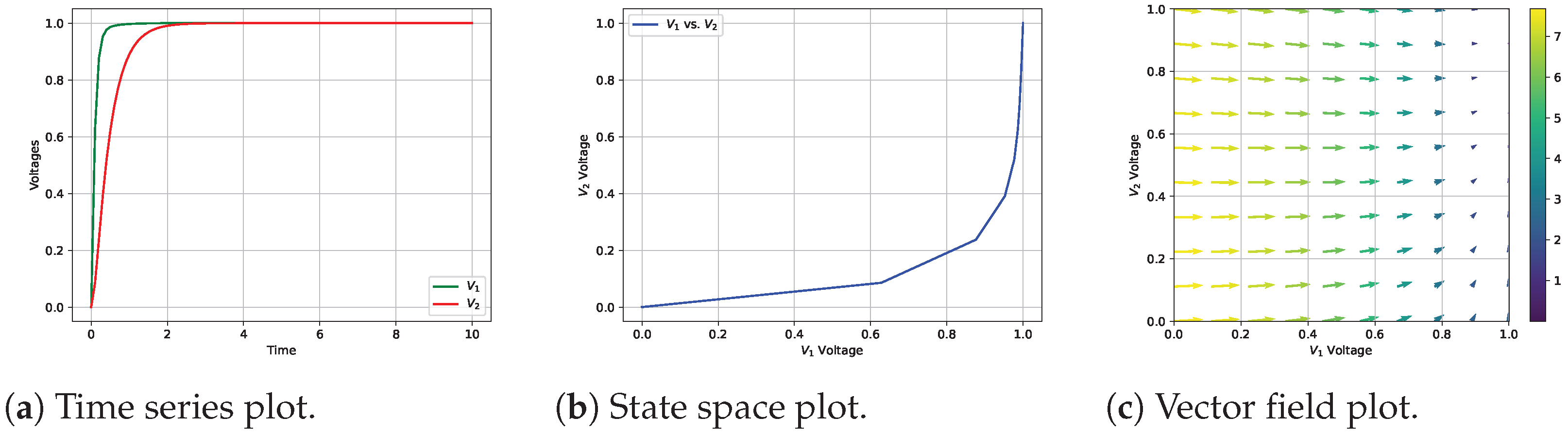
4.1. RC Circuit System
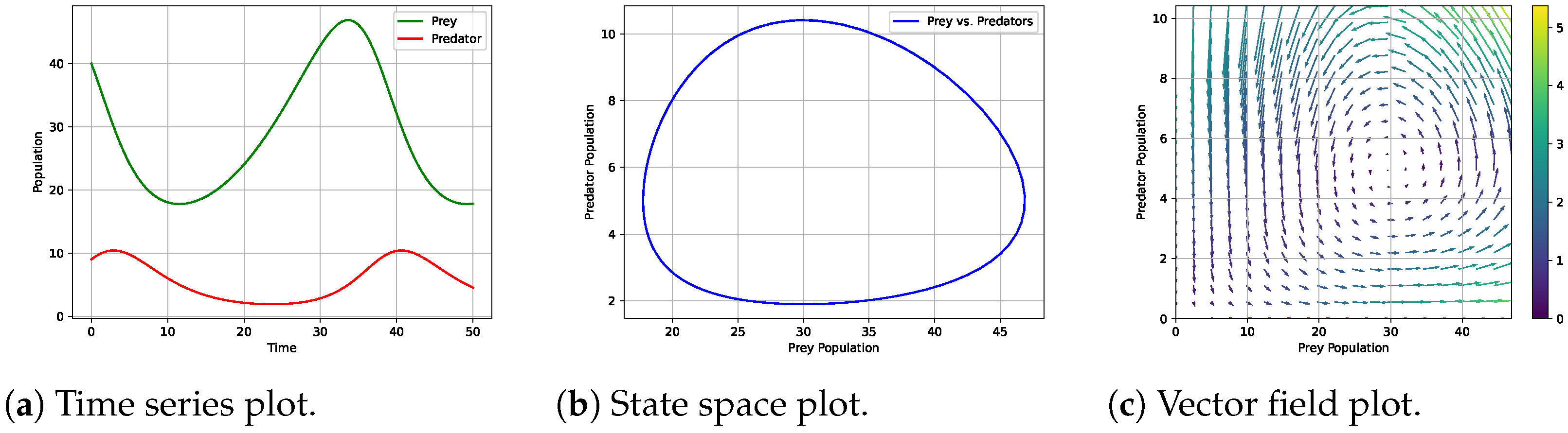
4.2. Lotka–Volterra Predator–Prey System
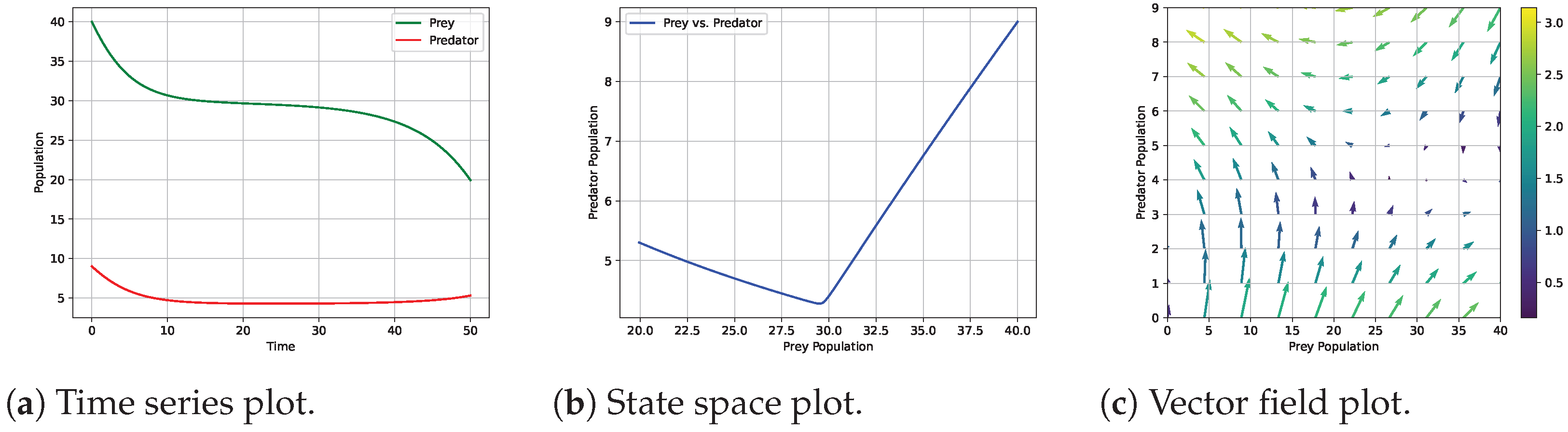
4.3. Chemical Reaction System
5. Conclusions
Author Contributions
Funding
Data Availability Statement
Conflicts of Interest
References
- Ibrahim, A.; Kashef, R.; Corrigan, L. Predicting Market Movement Direction for Bitcoin: A Comparison of Time Series Modeling Methods. Comput. Electr. Eng. 2021, 89, 106905. [Google Scholar] [CrossRef]
- Yemelyanov, V.; Chernyi, S.; Yemelyanova, N.; Varadarajan, V. Application of Neural Networks to Forecast Changes in the Technical Condition of Critical Production Facilities. Comput. Electr. Eng. 2021, 93, 107225. [Google Scholar] [CrossRef]
- Hornik, K.; Stinchcombe, M.; White, H. Multilayer Feedforward Networks Are Universal Approximators. Neural Netw. 1989, 2, 359–366. [Google Scholar] [CrossRef]
- Chen, R.T.; Rubanova, Y.; Bettencourt, J.; Duvenaud, D.K. Neural ordinary differential equations. In Proceedings of the 32nd International Conference on Neural Information Processing Systems, Montréal, QC, Canada, 3–8 December 2018; Volume 31. [Google Scholar]
- Xing, Y.; Ye, H.; Zhang, X.; Cao, W.; Zheng, S.; Bian, J.; Guo, Y. A Continuous Glucose Monitoring Measurements Forecasting Approach via Sporadic Blood Glucose Monitoring. In Proceedings of the 2022 IEEE International Conference on Bioinformatics and Biomedicine (BIBM), Las Vegas, NV, USA, 6–8 December 2022; pp. 860–863. [Google Scholar] [CrossRef]
- Su, X.; Ji, W.; An, J.; Ren, Z.; Deng, S.; Law, C.K. Kinetics Parameter Optimization via Neural Ordinary Differential Equations. arXiv 2022. [Google Scholar] [CrossRef]
- Laurie, M.; Lu, J. Explainable Deep Learning for Tumor Dynamic Modeling and Overall Survival Prediction Using Neural-ODE. arXiv 2023. [Google Scholar] [CrossRef] [PubMed]
- Dinh, P.; Jobson, D.; Sano, T.; Honda, H.; Nakamura, S. Understanding Neural ODE prediction decision using SHAP. In Proceedings of the 5th Northern Lights Deep Learning Conference (NLDL), Tromsø, Norway, 9–11 January 2024; Proceedings of Machine Learning Research. Lutchyn, T., Ramírez Rivera, A., Ricaud, B., Eds.; American Psychological Association: Washington, DC, USA, 2024; Volume 233, pp. 53–58. [Google Scholar]
- Gao, P.; Yang, X.; Zhang, R.; Huang, K.; Goulermas, J. Explainable Tensorized Neural Ordinary Differential Equations for Arbitrary-Step Time Series Prediction. IEEE Trans. Knowl. Data Eng. 2023, 35, 5837–5850. [Google Scholar] [CrossRef]
- Minh, D.; Wang, H.X.; Li, Y.F.; Nguyen, T.N. Explainable Artificial Intelligence: A Comprehensive Review. Artif. Intell. Rev. 2022, 55, 3503–3568. [Google Scholar] [CrossRef]
- Rajput, S.; Kapdi, R.; Raval, M.; Roy, M. Interpretable Machine Learning Model to Predict Survival Days of Malignant Brain Tumor Patients. Mach. Learn. Sci. Technol. 2023, 4, 025025. [Google Scholar] [CrossRef]
- Rojat, T.; Puget, R.; Filliat, D.; Del Ser, J.; Gelin, R.; Díaz-Rodríguez, N. Explainable Artificial Intelligence (XAI) on TimeSeries Data: A Survey. arXiv 2021. [Google Scholar] [CrossRef]
- Elsonbaty, A.; Elsadany, A.A. On Discrete Fractional-Order Lotka-Volterra Model Based on the Caputo Difference Discrete Operator. Math. Sci. 2023, 17, 67–79. [Google Scholar] [CrossRef]
- Coelho, C.; Costa, M.F.P.; Ferrás, L.L. Synthetic Chemical Reaction. 2023. Available online: https://www.kaggle.com/datasets/cici118/synthetic-chemical-reaction (accessed on 20 November 2023).
- Coelho, C.; Costa, M.F.P.; Ferrás, L.L. A Two-Stage Training Method for Modeling Constrained Systems With Neural Networks. J. Forecast. 2025. [Google Scholar] [CrossRef]


Disclaimer/Publisher’s Note: The statements, opinions and data contained in all publications are solely those of the individual author(s) and contributor(s) and not of MDPI and/or the editor(s). MDPI and/or the editor(s) disclaim responsibility for any injury to people or property resulting from any ideas, methods, instructions or products referred to in the content. |
© 2025 by the authors. Licensee MDPI, Basel, Switzerland. This article is an open access article distributed under the terms and conditions of the Creative Commons Attribution (CC BY) license (https://creativecommons.org/licenses/by/4.0/).
Share and Cite
Coelho, C.; da Costa, M.F.P.; Ferrás, L.L. XNODE: A XAI Suite to Understand Neural Ordinary Differential Equations. AI 2025, 6, 105. https://doi.org/10.3390/ai6050105
Coelho C, da Costa MFP, Ferrás LL. XNODE: A XAI Suite to Understand Neural Ordinary Differential Equations. AI. 2025; 6(5):105. https://doi.org/10.3390/ai6050105
Chicago/Turabian StyleCoelho, Cecília, Maria Fernanda Pires da Costa, and Luís L. Ferrás. 2025. "XNODE: A XAI Suite to Understand Neural Ordinary Differential Equations" AI 6, no. 5: 105. https://doi.org/10.3390/ai6050105
APA StyleCoelho, C., da Costa, M. F. P., & Ferrás, L. L. (2025). XNODE: A XAI Suite to Understand Neural Ordinary Differential Equations. AI, 6(5), 105. https://doi.org/10.3390/ai6050105