ARM-IRL: Adaptive Resilience Metric Quantification Using Inverse Reinforcement Learning

Abstract

Background/Objectives: The resilience of safety-critical systems is gaining importance due to the rise in cyber and physical threats, especially within critical infrastructure. Traditional static resilience metrics may not capture dynamic system states, leading to inaccurate assessments and ineffective responses to cyber threats. This work aims to develop a data-driven, adaptive method for resilience metric learning. Methods: We propose a data-driven approach using inverse reinforcement learning (IRL) to learn a single, adaptive resilience metric. The method infers a reward function from expert control actions. Unlike previous approaches using static weights or fuzzy logic, this work applies adversarial inverse reinforcement learning (AIRL), training a generator and discriminator in parallel to learn the reward structure and derive an optimal policy. Results: The proposed approach is evaluated on multiple scenarios: optimal communication network rerouting, power distribution network reconfiguration, and cyber–physical restoration of critical loads using the IEEE 123-bus system. Conclusions: The adaptive, learned resilience metric enables faster critical load restoration in comparison to conventional RL approaches.

1. Introduction

The threat of cyber attacks in the energy sector has been increasing worldwide during the last few decades. Though these events are probabilistically rare, they can cause significant impacts to the grid. To make the electric grid resilient to cyber threats, it is essential to identify appropriate resilience metrics. These metrics can be leveraged to develop response and recovery strategies that account for both the cyber and physical component of the grid. Resilience is defined as the ability of a system to withstand adverse events while maintaining the critical functionalities of the system [1]. Physical resilience metrics in the literature tend to be static, or evaluated post-event. The authors in [2] classify resilience metrics to be either attribute based, or performance based. Attribute based metrics are generally static in nature, as the electric grid components are not frequently changed. Performance-based metrics tend to be evaluated post-events or predicted based on historical performance. Both types of metrics are not sufficient to guide operators towards decisions that enable real-time resilience.

On the cyber side, the cyber resilience metric heavily depends on the intrusion stage in the cyber kill chain [3]. With the proliferation of security sensors for cyber intrusion detection, various kinds of resilience indices are formulated from system logs, control process data, and alerts from monitoring systems [4]. Cyber resilience metrics have been reported along physical, information, social, and cognitive verticals by the authors in [5]. While individual qualitative and quantitative measures suffice to understand system state in a localized manner, they rarely provide actionable information to ensure resilience at a global or system level.

In previous work, the authors [6,7] designed resilience metrics for transmission and distribution systems. These metrics are computed in real-time based on system properties and measurements using a multi-criteria decision-making approach. Methods such as the analytical hierarchical process, successive Pareto optimization, and Choquet Integral among others can be considered, but these methods become harder to scale as the objective space increases [8].

Designing an adaptive resilience metric can help in identifying optimal actions, in a multi-domain problem space such as cyber–physical systems, by maximizing a single objective function rather than a weighted sum of mixed objectives. This work proposes a novel approach to identifying a state- and time-dependent adaptive resilience metric. The motivation for the approach comes from the paper [9], which discusses the fourth stage of the cyber-resilient mechanism, the response mechanism, which creates a dynamic process involving information extraction, online decision making, and security reconfiguration. Reinforcement learning (RL) enables the development of response policies that adapt to the dynamic observations. Unlike the conventional classic control approaches, which involves modeling, design, testing, and execution, RL involves training, testing, and execution [9]. Hence, we approach the process of identifying an adaptive resilience metric using the RL framework not by learning optimal decisions but rather by learning the objective function.

The major contributions of this work include the following:

• Leveraging IRL for quantifying adaptive resilience metrics for optimal network routing, distribution feeder network reconfiguration, and a combined cyber–physical critical load restoration problem.
• Evaluating a heuristic approach for expert demonstrations that are required for imitation learning-based policy development such as IRL.
• Assessing the effectiveness of adversarial inverse reinforcement learning (AIRL) alongside imitation learning and other IRL variants across different problem scenarios and network sizes. Evaluation criteria include the episode lengths required for an agent to achieve its goal.
• Explaining the learned resilience function by visualizing them as a function of selected state and action pairs.

The rest of this paper is organized as follows: Section 2 provides a brief review of various cyber–physical resilience metrics along with the application of RL in network reconfiguration. Section 3 presents the formulation of three Markov Decision Process (MDP) problems and introduces the notion of adaptive resilience metric learning. Section 4 proposes the use of IRL to learn the adaptive resilience metric and then to further use it to learn the optimal policy. The system architecture for obtaining expert trajectories followed by the resilience metric to find the optimal policy are presented in Section 5. In Section 6, the imitation and IRL learning techniques are evaluated for finding the optimal policies for rerouting, network reconfiguration, and combined cyber–physical critical load restoration problems.

2. Background

Prior work on different resilience metrics considered in cyber–physical power systems is presented here. This section also briefly introduces how RL and specifically IRL can be considered for the adaptive learning of a unique resilience metric.

2.1. Cyber, Physical, and Cyber–Physical Resilience Metrics

There are different classes of cyber resilience metrics, such as topological, investments, and risks. The types of metrics crucial for responding to an event depend on the threat model, the physical domain that the cyber infrastructure supports, the scale of the system, and the stage of intrusion. Moreover, the evaluation of such metrics takes time and effort due to investment in specialized applications to gather data from different sensors, such as Security Information and Event Management, Intrusion Detection Systems, and system logs. To improve cyber resilience, Ref. [10] suggests microsegmentation with the goal of slowing down cyber intruders locally as they initiate their navigation into the system. There are numerous other cyber metrics, for instance, topological metrics that comprise path redundancy and node and edge betweenness centrality [7]. Rather than considering a variety of metrics, this study concentrates on acquiring a single adaptive metric that amalgamates various resilience metrics.

For operational and physical system resilience—specifically in power grids—a resilience trapezoid approach is used to evaluate system response to an event [11]. This approach is based on multiple metrics, such as how quickly and how significantly resilience drops, the extent of the post-event degraded state, and how promptly the network recovers to the pre-event resilient state. For the transmission network, the suggested scoring methods include the number of lines outages and restored per hour, the number of lines in service, etc. For a distribution grid, the priority varies because the network is radial, and prioritizing service to the critical loads far from the transmission grid substation is more essential. The authors of [12] propose the formation of a networked and dynamic microgrid to enhance resilience during major outages through proactive scheduling, feasible islanding, outage management, etc., depending on the event occurrence probability and clearance times. The authors of [13] propose an optimal resilient networked microgrid scheduling scheme using Bender’s decomposition and evaluating them based on varying topologies of microgrid interconnection. Resilience is system dependent, and needs to account for user preferences. Hence, authors have often used weights to quantify impact for different parameters and factors [14]. Our proposed approach also solves a similar problem of identifying a common metric but by learning a reward function in the Markov Decision Process (MDP) model, through IRL, which is discussed in detail in Section 4.

Researchers have also focused on inter-domain resilience metric computation. For instance, Ref. [15] proposes thermal power generator system resilience quantification with respect to water scarcity and extreme weather events. Similarly, Ref. [16] proposes a novel approach based on RL for optimal decision making using interdependence between different sectors, e.g., agriculture, energy and water systems. The authors of [17] propose a performance-based cyber-resilience metric quantification, through a Linear Quadriatic Regulator-based control technique, to balance the systematic impact. In the paper, one of the metrics, named the systematic impact metric, that computes the fraction of the network host that is not infected and the rate at which the scanning worm infects hosts are considered. For the total recovery effort, a fraction of sent packets is dropped and retransmitted, and the average round-trip times are considered. The metrics are evaluated by incorporating moving target defense against the reconnaissance attack. The authors of [1] propose a methodology to extract resilience indices from syslogs and process data from a real wastewater treatment plant while simulating diverse threats targeting critical feedback control loops in the plant. A Cyber–Physical Systems (CPS) resilience metric framework that evaluates resilience, dependent on performance indicators, and identifies the reason for good or bad resilience metric is presented in [18]. But all these works make use of static formulation for defining a resilience metric.

2.2. Adaptive Resilience Metric Learning Using RL

Recently, data-driven control methods, especially RL, have been applied to decision support and control in power system applications. These applications range from voltage control [19], frequency control, and energy management systems such as Optimal Power Flow (OPF) [20], to electric vehicle charging scheduling, battery management, and residential load control [21]. For OPF, the RL agent considers a fixed reward, such as the minimization of the total cost of operation. Similarly for a network router’s rerouting problem, the minimization of delay or reducing packet drop rates between the sender and receiver is given a higher reward. For resilience, a single cost function might not always capture the true preferences of the operator. This is because there could be other factors the operator cares about, such as grid reliability, cyber–physical security, or environmental concerns.

Resilience metrics that can be leveraged for response and recovery depend on multiple factors, such as cost, time, impact on systems, and redundant paths between transceivers or between the load and generators. Recently, an unsupervised artificial neural network variant, called a self-organizing map [22], was proposed for the resilience quantification and control of distribution systems under extreme events. Although our previous approach [7] considered both cyber and physical resilience metrics, it is not adaptive. The second approach [22] is adaptive, but it has only been evaluated on a non-cyber-enabled distribution feeder. In this work, we propose a novel approach, where IRL is used to learn the resilience metric while also learning the control policy in parallel. This is a first of a kind work that validates the efficacy of using IRL against the conventional RL approach for enhancing resilience in a cyber–physical environment. The next section introduces the problem formulation and the IRL approach in detail.

2.3. Imitation and Inverse Reinforcement Learning

In the area of cybersecurity, imitation learning and IRL are considered. For instance, Ref. [23] proposes the idea of using Generative Adversarial Imitation Learning (GAIL) for intelligent penetration testing, where they construct expert knowledge bases by collecting state–action pairs from successful exploitations of pretrained RL models. Similarly, Ref. [24] compare the model-free learning approaches with imitation learning for penetration testing and validate that injecting prior knowledge through expert demonstrations makes the training efficient. But there has been no prior research on leveraging IRL or imitation learning for incident response, which our current work is focusing on.

Similarly, in the area of power systems, there have been many use cases that leverage imitation learning and IRL. An imitation Q-learning-based energy management system is designed in this paper [25] to reduce battery degradation and improve energy efficiency for the electric vehicle. Similarly [26] leverages behavioral cloning and DAgger algorithms for optimal power dispatch, reducing transmission overloading and balancing power. Unlike these work, our work is focused on critical load restoration after there is a line outage contingency with and without cyber attacks, which is a challenging problem addressed by the previous researcher.

3. Problem Formulation

To effectively model optimization problem such as router rerouting in communication networks, distribution grid network reconfiguration and the combination of both controls in power systems, the Markov Decision Process (MDP) framework offers a powerful, unified approach. These three problems involve making a sequence of interdependent decisions—such as selecting alternate paths for data packets or switching network branches—to optimize performance metrics like latency, reliability, or power loss. By framing these as MDPs, the system state (e.g., current topology and voltage profile of the load) evolves based on the agent’s actions (e.g., reroute or reconfigure), and a reward function guides the agent toward desirable outcomes. Before delving into the MDP of the three problems, we introduce what is a MDP.

3.1. Markov Decision Process (MDP)

An MDP is a discrete-time probabilistic model that captures the interactions between an agent and its environment. The goal is to make optimal decisions—such as operating sectionalizing switches for load restoration or adjusting routing strategies to counter cyber threats. In this context, agents serve as decision-making units, while the environment represents the current condition of the cyber–physical system. An MDP is characterized by five elements: a set of states (S), a set of actions (A), a transition function $P\left(s_{t+1}\right|s_t,a_t)$ that models how actions affect future states, a reward function $R\left(s_{t+1}\right|s_t,a_t)$ that assigns feedback for actions taken, and a discount factor $\gamma$ that weighs future rewards.

3.1.1. MDP 1: Optimal Rerouting

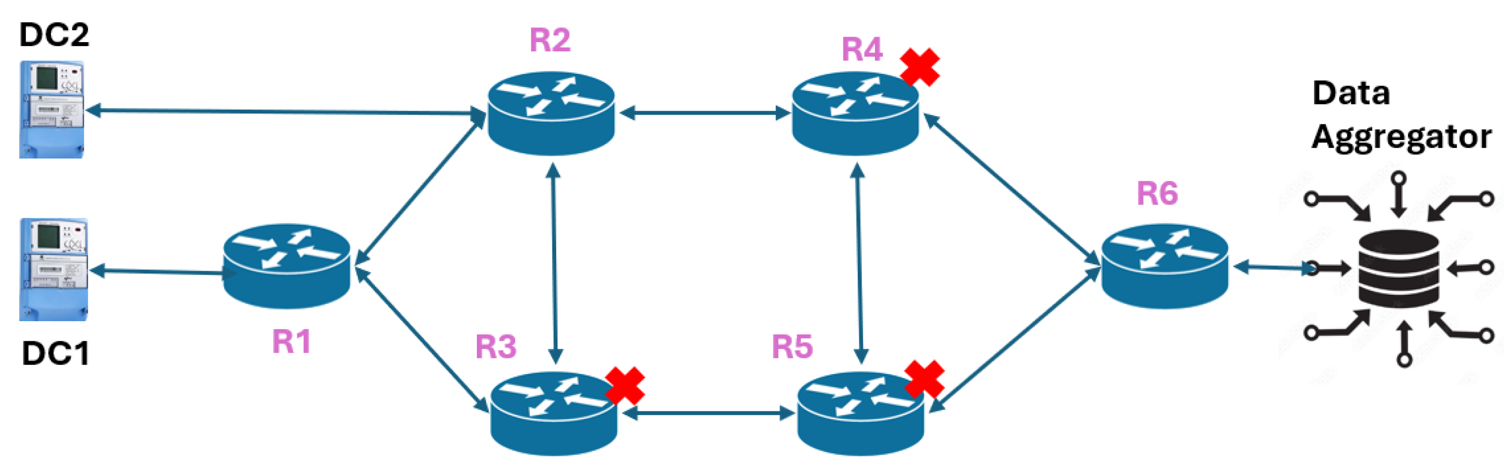
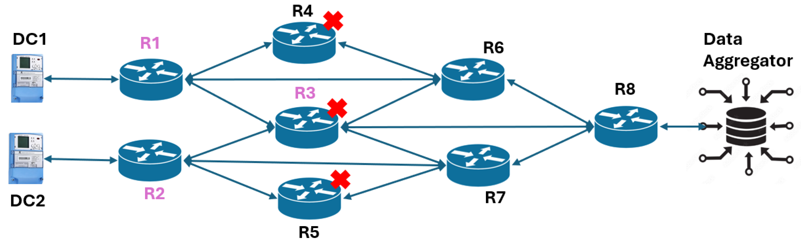
The goal of this experiment is to leverage the cyber resilience metric learning approach to re-route the traffic between the Data Concentrators (DCs) of the respective zones and the Data Aggregator (DA) within the least number of steps in an episode. The DC acts as a data collector and forwarder for all the smart meters in the zones. When a fault occurs in the distribution feeder, the relay captures it and forwards it to the DC. The DC within the zone forwards the state to the Distribution System Operator (DSO), which acts as the DA. Two different-sized cyber networks under study comprise six routers (Figure 1) and eight routers (Figure 2) respectively. The MDP model for the re-routing problem is given by the following:

• Observation Space: The system states are the packet drop rates at every router and the channel utilization rate $U_r$ at every channel.
• Action Space: The actions within the discrete action MDP depend on the action at every router to select the highest-priority nearest hop among all the neighbors. There are two $MultiDiscrete$ action models considered: (a) $MultiDiscrete$$\{N_r,N_{inf}\}$, and (b) $MultiDiscrete$${\left\{N_{inf}\right\}}^{\left\{N_r\right\}}$, where $N_r$ is the # of controllable routers and $N_{inf}$ is the # of interfaces of a router with other routers. In Figure 1 and  Figure 2, the routers with a lilac legend represent the controllable routers. In the first type of action space, for a given step, only one router is selected to change the route, while in the second type, all the controllable router’s routing path is altered. In the first network (Figure 1), for a given step in an RL episode, any one of routers $R1$ to $R6$ is selected to modify the static route. For the second network (Figure 2), all three controllable routers $R1$, $R2$, and $R3$ change the route in a given step. Hence, the action space for the first network is MultiDiscrete $\{6,3\}$, while for the second network it is MultiDiscrete $\left\{\right\{3\},\{3\},\{3\left\}\right\}$. In every episode, any one of the routers from $R_{comp}$ = $\{R3,R4,R5\}$ is compromised. The goal of the agent is to ensure secure packet transmission between the DCs and the DA.
• Reward Model: The reward is based on the number of packets successfully received at the destination, with additional consideration for average latency, which includes queuing and transmission delays influenced by channel bandwidth and router queue size, while assuming fixed propagation delay, based on our prior work [27].
• Termination Criteria: The episode in this MDP is terminated when at least $N_g$ packets are successfully received at the DA from the DC of the corresponding zones.
• Threat: A Denial of Service (DoS) attack is performed at a set of routers in the network as illustrated in Figure 1 and  Figure 2.

3.1.2. MDP 2: Distribution Feeder Network Reconfiguration

The goal of this experiment is to leverage the resilience metric learning approach to restore the critical loads such as hospital, fire station, etc., within the least number of transitions in an episode, to prevent major implications. To execute the contingencies and restore them using distribution feeder network reconfiguration with a sectionalizing switch, we use an automated switching device that is intended to isolate faults and restore loads. The optimal network reconfiguration is modeled as an MDP. Variability is introduced at the beginning of each episode through the random selection of different load profiles along with a contingency since the agent needs to learn to restore the system from any contingencies and loading factors. The detail MDP model with the observation, action, reward and terminating criteria is based off the network configuration modeled in our prior work [27].

3.1.3. MDP 3: Combined Cyber and Physical Restoration of Critical Load

The objective of the combined cyber–physical critical load restoration problem is to restore the critical loads in the distribution grid, and the $N_g$ packets from the DC are successfully received at the DA. The cyber–physical co-simulation uses shared Python queue objects across threads to synchronize events between the SimPy-based cyber and OpenDSS-based physical environments [27]. Control actions and cyber threats are exchanged via $Phy-Cyb-Queue$ and $Cyb-Phy-Queue$, enabling dynamic interactions such as command execution or failure due to cyberattacks. The observation and action spaces from the rerouting and network reconfiguration environments are concatenated, while the rewards from both environments are combined through addition. The goal is reached when both the cyber and physical goals are achieved. It is relatively harder to reach a combined goal since the dynamics of both cyber and physical domains are different except for the message passing using the queues. For improvement in performance, the reward model is modified as such:

$$R_{cp}=\left\{\begin{array}{cc}{R}_c+R_p\hfill & \mathrm{if}{G}_c\wedge G_p\hfill \\ R_p\hfill & \mathrm{if}{G}_c\wedge \overline{G_p}\hfill \\ R_c\hfill & \mathrm{if}\overline{G_c}\wedge G_p\hfill \end{array}\right.$$

(1)

where $G_c$ and $G_p$ are the Boolean representing the goal state reached status. The rationale behind such reward engineering is due to preventing a higher reward being given to the agent when it has reached only one goal.

The combined environment is further examined to test if it follows the Markov property. Suppose there are two Markov chains: $X_t$ for the MDP1 (cyber) and $Y_t$ for the MDP2 (physical). Each of them satisfies the Markov property individually:

$$\left\{\begin{array}{c}P\left(X_{t+1}\right|X_t,X_{t-1},\dots ,X_0)=P\left(X_{t+1}\right|X_t)\hfill \\ P\left(Y_{t+1}\right|Y_t,Y_{t-1},\dots ,Y_0)=P\left(Y_{t+1}\right|Y_t)\hfill \end{array}\right.$$

(2)

Defining the joint process $Z_t=(X_t,Y_t)$, we need to show that $P\left(Z_{t+1}\right|Z_t,Z_{t-1},\dots Z_0)=P\left(Z_{t+1}\right|Z_t)$. In this regard, we will monitor the transition probability:

$$P(X_{t+1},Y_{t+1}|X_t,Y_t,\dots ,X_0,Y_0)$$

(3)

If the transitions for X and Y depend only on their current state and optionally each other’s current state but not on the past states, then:

$$P(X_{t+1},Y_{t+1}|X_t,Y_t,\dots )=P(X_{t+1},Y_{t+1}|X_t,Y_t)$$

(4)

which satisfies the Markov property for the joint process $Z_t$. This property is proved empirically by following these three steps: (a) Run episodes from both the gym environments. (b) Track the joint states and transitions (Algorithm 1). (c) Finally, check the empirical probability distribution of the next state given: (1) only the current state, and (2) the full history. If the probabilities are approximately computed to be the same as the divergence, then it satisfies the Markov property, i.e., if the variable $avg\_diff$ in Algorithm 2 returns zero or a very low value. By collecting transition for 100 episodes for the MDP3 and running Algorithm 2, we obtain the $avg\_diff$ to be 0.00017.

3.2. Inverse Reinforcement Learning

Conventionally, it is easy to obtain an optimal sequence of actions in an MDP when the reward function is static, but it is difficult to design the reward function and its parameters when there are multiple resilience metrics to consider. Adaptively learning the important resilience metrics depends on operator inputs rather than purely relying on the data, such as bus voltages and phases.

Why use inverse reinforcement learning (IRL) for designing adaptive resilience metrics? The main idea in IRL is to learn the weights as a function of time t and system states s, while i indicates the type of metric, such as diversity, response time, response cost, and impact. If the model is known, then state s is a function of time. Both linear and neural network-based approaches of function approximations of the reward are formulated in the literature. Equation (5) is the linear variant of learning an adaptive resilience metric:

$$R_{adapt}(t,s)=\sum _i{w}_i(t,s)R_i(t,s)$$

(5)

Algorithm 1 Run combined environments and collect transitions

1: procedure run_combined_envs($cyb\_env$, $phy\_env$, $episodes$, $max\_steps$)  2:     $transitions\leftarrow \mathrm{defaultdict}\left(\mathrm{defaultdict}\right(int\left)\right)$  3:     $history\_transitions\leftarrow \mathrm{defaultdict}\left(\mathrm{defaultdict}\right(int\left)\right)$  4:     for $episode\leftarrow 1$ to $episodes$ do  5:         $X_t\leftarrow cyb\_env.reset\left(\right)$  6:         $Y_t\leftarrow phy\_env.reset\left(\right)$  7:         $Z_{t-1}\leftarrow None$  8:         for $step\leftarrow 1$ to $max\_steps$ do  9:            $action1\leftarrow \mathrm{sample}\mathrm{from}cyb\_env.action\_space$ 10:            $action2\leftarrow \mathrm{sample}\mathrm{from}phy\_env.action\_space$ 11:            $X_{t+1},\_,done1\leftarrow cyb\_env.step\left(action1\right)$ 12:            $Y_{t+1},\_,done2\leftarrow phy\_env.step\left(action2\right)$ 13:            $Z_t\leftarrow (X_t,Y_t)$ 14:            $Z_{t+1}\leftarrow (X_{t+1},Y\_t+1)$ 15:            $transitions\left[Z_t\right]\left[Z_{t+1}\right]+=1$ 16:            if $Z_{t-1}\ne None$ then 17:                $history\_state\leftarrow (Z_{t-1},Z_t)$ 18:                $history\_transitions[history\_state]\left[Z_{t+1}\right]+=1$ 19:            end if 20:            $Z_{t-1}\leftarrow Z_t$ 21:            $X_t\leftarrow X_{t+1}$ 22:            $Y_t\leftarrow Y_{t+1}$ 23:            if $done1$ or $done2$ then 24:                break 25:            end if 26:         end for 27:     end for 28:     $cyb\_env.close\left(\right)$ 29:     $phy\_env.close\left(\right)$ 30:     return $transitions,history\_transitions$ 31: end procedure

Algorithm 2 Check combined Markov property

1: Input: $transitions$, $history\_transitions$, $top\_k$  2: Output:  $avg\_diff$  3: $divergences$ = []  4: for $history\_state$ in $history\_transitions$ (up to top_k) do  5:     $history\_next\_probs$ = NormalizeCounts($history\_transitions$[$history\_state$])  6:     $curr\_next\_probs$ = NormalizeCounts($transitions[current\_state]$)  7:     $diff$ = $\sum |history\_next\_probs-curr\_next\_probs|$  8:     $divergences$.append($diff$)  9: end for 10: $avg\_diff$ = mean($divergences$) return $avg\_diff$

The notion of time is integrated based on the RL framework because it is a sequential decision-making framework, whereas resilience dependency on state can be incorporated using IRL. The IRL problem in a combined environment encounters multiple objectives, where the notion of aggregation helps in merging these multiple objectives into a single scalar reward that can be used for policy optimization. Aggregating multiple reward functions allow for more general models that are adaptable to different scenarios that are tweaked through the weights. Unlike the linear variant of aggregation in Equation (5), this work has focused on leveraging the neural network variant, where the weights are learned.

In IRL, the agents infer the reward functions from expert demonstrations. Expert demonstration refers to the process of using the behavior of an expert agent (or demonstrator) to infer the reward function that the expert is assumed to be optimizing. The challenges in using IRL are (a) an under-defined problem (where problem formulation makes it hard to formulate a single optimal policy and reward function), (b) difficulty in interpreting and implementing a metric learned through IRL, and (c) the fact that expert demonstrations which drive IRL might not be always optimal. Usually, this area is adopted when an agent has an extremely rough estimate of the reward function/performance metric. IRL has also been proven to be less affected by the dynamics of the underlying MDP (when the reward is simple or the dynamics change, IRL outperforms apprenticeship learning). Before discussing various approaches of IRL, first, we define the MDP for the three problems that will be solved.

4. Proposed Solutions and Their Variants

An ideal IRL goal is to learn rewards that are invariant to changing dynamics. Similarly, our goal is to learn a single adaptive resilience metric that is invariant to types of threats and contingencies. Few prior works have leveraged IRL in the area of security, such as learning attacker behavior using IRL [28]. Though IRL methods are difficult to apply to large-scale, high-dimensional problems with unknown dynamics, they still hold promise for automatic reward acquisition; hence, this work focuses on leveraging various methods of IRL and imitation learning techniques. In addition to learning an adaptive metric, this work also evaluates the performance of the learned policy based on the number of steps an agent takes to reach the goal state.

4.1. Inverse Reinforcement Learning (IRL)

IRL is a variant of imitation learning, which is preferred when learning the reward functions from demonstrations is statistically more efficient than directly learning the policy. Imitation learning is useful when it is easier for a demonstrator to show the desired behavior rather than to specify a reward model that would generate the same behavior. It is also useful when directly learning the policy, as in forward RL, is more challenging. The other imitation learning techniques considered in this work include behavioral cloning, interactive direct policy learning, Data Aggregator (DAgger), and Generative Adversarial Imitation Learning (GAIL). A generic approach in defining an IRL problem and solving it, is illustrated here:

• Consider an MDP without the reward $(S,A,\gamma ,P)$.
• Given the demonstration from an expert, e.g., the trajectories generated according to expert policy $D=(s_0^i,a_0^i,s_1^i,a_1^i,\dots ,s_t^i,a_t^i,\dots ),i=1,\dots ,n,a_t^i\sim {\pi }_e\left(s_t^i\right)$
• The assumption is that the expert is using the optimal policy with respect to a reward function, e.g., R, which is unknown to us:

  $${\pi }_e={\pi }^{\ast }=\underset{\pi }{arg\; max}E[\sum _{t=0}^{\infty }{\gamma }^{t}R(s_t,\pi \left(s_t\right))]$$

  (6)
• The IRL objective is then to infer R and use that to recover the expert policy.
• First, it is assumed that the true reward function is in the form of $R\left(s\right)={\left(w^{\ast }\right)}^T\varphi \left(s\right)$, where $\varphi$ is a feature considered in the state space, and goal is to find $w^{\ast }$.
• States in the MDP can be represented as features. Define the feature expectation $\mu$ as, for a given feature, $\varphi$, the ${\mu }_{\pi }^{\varphi }\left(s\right)=E_{\pi }\left[{\sum }_{t=0}^{\infty }{\gamma }^t\varphi \left(s_t\right)|s_0=s\right]$.
• Given the policy $\pi$, the value function $V_{\pi }\left(s\right)=E_{\pi }\left[{\sum }_{t=0}^{\infty }{\gamma }^t{w}^T\varphi \left(s_t\right)|s_0=s\right]=w^T{\mu }_{\pi }^{\varphi }\left(s\right)$.
• Optimal policy, ${\pi }^{\ast }$, requires $V_{{\pi }^{\ast }}\ge V_{\pi },\forall \pi$.
• Hence, one can find the optimal $w^{\ast }$ that satisfies ${\left(w^{\ast }\right)}^T({\mu }_{\pi }^{{\varphi }^{\ast }}\left(s\right)-{\mu }_{\pi }^{\varphi }\left(s\right)),\forall \pi$, which can have infinite solutions; thus, how do we obtain a unique optimal solution? That gives rise to different IRL techniques in that literature that we will discuss further.

The IRL algorithms are broadly categorized into three types, per the review paper [29]: 1. Max-Margin Method: The max-margin method is the first class of the IRL method, where the reward is considered to be the linear combination of features and attempts to estimate the weights associated with the features. It estimate the rewards that maximize the margin between the optimal policy or value function and all other policies or value functions. 2. Bayesian IRL: The Bayesian IRL [30] targets a learning function that maximizes the posterior distribution of the reward. The advantage of the Bayesian method is the ability to convey the prior information about the reward through a prior distribution. Another advantage of using the Bayesian IRL is the ability to account for complex behavior by modeling the reward probabilistically as a mixture of multiple resilient functions. 3. Maximum Entropy: This variant will be discussed in detail as an extension to imitation learning. Interested readers who would like a deeper understanding of the algorithms are referred to the next subsection.

4.2. Imitation Learning

Before discussing the proposed IRL technique, we present a few imitation learning techniques that have been precursors to the development of AIRL. A typical approach to imitation learning is to train a classifier or regressor to predict an expert’s behavior given the training data of the encountered observations (input) and actions (output) performed by the expert. Some imitation learning techniques that are considered for evaluation in this work are as follows:

4.2.1. Behavioral Cloning

In behavioral cloning (BC), an agent receives as training data both the encountered states and actions of the expert and then uses a regressor to replicate the expert’s policy. The steps involved in BC include the following: (a) Collect demonstrations from expert. (b) Assuming that the expert trajectories are independent and identically distributed (i.i.d.) state–action pairs, learn a policy ${\pi }_{\theta }$ using supervised learning by minimizing the loss function $L(a^{\ast },{\pi }_{\theta }\left(s\right))$, where $a^{\ast }$ is the expert’s action.

4.2.2. DAgger

Due to the i.i.d. assumption in the behavior cloning, if a classifier makes a mistake, e.g., with probability, $ϵ$, under the distribution of states faced by the demonstrator, then it can also make as many as $T^2ϵ$ mistakes, averaged over T steps under the distribution of states the classifier enforces, resulting in compounded errors [31]. A few prior approaches addressed the issue in reducing the error to $Tϵ$ but still resulted in a non-stationary policy. DAgger starts by extracting a data set at each iteration under the current policy and trains the next policy under the aggregate of all the collected data sets. The intuition behind this algorithm is that over the iterations, it is building up the set of inputs that the learned policy is likely to encounter during its execution based on previous experience (training iterations). This algorithm can be interpreted as a follow-the-leader algorithm, in that at iteration n, one picks the best policy ${\widehat{\pi }}_{n+1}$ in hindsight, i.e., under all trajectories seen so far over the iterations. The pseudo code for the DAgger algorithm is presented in Algorithm 3.

Algorithm 3 DAgger pseudo code [31]

1: Initialize the trajectory accumulator D. 2: Initialize the first estimate of a policy, $\widehat{{\pi }_1}$. 3: for i = 1 to N do 4:     Update ${\pi }_i={\beta }_i{\pi }^{\ast }+(1-{\beta }_i)\widehat{{\pi }_1}$. 5:     Sample trajectories using ${\pi }_i$. 6:     Get the data set, $D_i=(s,{\pi }^{\ast }\left(s\right))$, of visited states by ${\pi }_i$ and actions from the expert. 7:     Aggregate data set $D=D\bigcup D_i$. 8:     Train classifier $\widehat{{\pi }_{i+1}}$ on D. 9: end for

4.2.3. Maximum Causal Entropy (MCE)

Due to uncertainties in cyber events, there is a need for addressing uncertainty in imitation learning. Hence, this approach adopts the principle of maximum entropy. Here, the reward is learned based on feature expectation matching. The reward model considered is the linear combination of the feature expectation with the optimal weights obtained, e.g., $\widehat{\theta }$. But numerous choices of $\widehat{\theta }$ can generate policy $\pi$ with the same expected feature counts as the expert, resulting in addressing the new challenge of breaking ties between same rewards. Hence, an extension of maximal entropy, Maximum Causal Entropy (MCE) is considered. Based on MCE, two major directions using a generative adversarial network (GAN) frameworks are developed: GAIL [32] and AIRL [33].

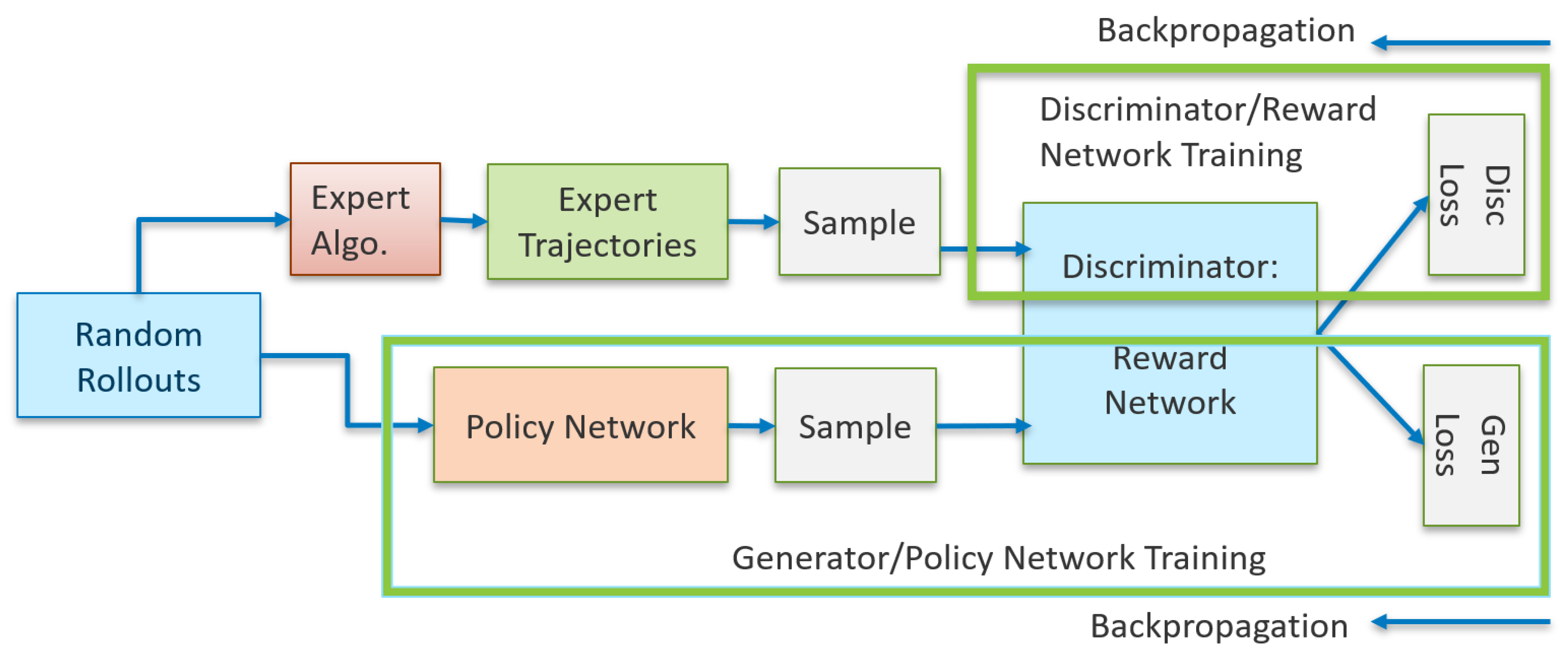
4.2.4. Generative Adversarial Imitation Learning (GAIL)

Before introducing the notion of the GAN framework within the IRL space, we present brief fundamentals on GANs. GANs are neural networks that learn to generate realistic samples of data on which they are trained. They are a generative model consisting of two networks: (a) generator and (b) discriminator, where the generator tries to fool the discriminator by generating fake, real-looking images (images are mentioned here because GANs were first applied in this domain). The discriminator tries to distinguish between real and fake images, while the generator’s objective is to increase the discriminator’s error rate. The GAN framework in the imitation learning harnesses the generative adversarial training to fit the states and actions distributions from the expert demonstrations [32]. To further clarify, the generator network produces actions trying to mimic the behavior of the expert demonstrator. Hence, the generator is the agent’s policy network, learning to take actions that will make its behavior as close as possible to the expert’s behavior, while the discriminator’s role is to distinguish between the behavior of the generator (the agent) and the expert. Hence, essentially in GAIL, the discriminator learns a reward function that reflects how “good” the agent’s actions are compared to the expert’s actions. The discriminator’s output is interpreted as a reward signal for the agent, guiding the policy to improve.

Like the feature expectation matching problem introduced in MCE, here, we discuss the expert’s state action occupancy measure matching problem [32]. Here, the IRL is formulated as the dual of the occupancy measure matching problem, where the induced optimal policy is obtained after running the forward RL. This process is exactly the act of recovering the primal optimum from the dual optimum, i.e., optimizing the Lagrangian with the dual variables fixed at the dual optimum values. The strong duality indicates that the induced optimal policy is the primal optimum and hence matches the occupancy measures with the expert. In this view, the IRL can be considered a method that aims to induce a policy that matches the expert’s occupancy measure.

The optimal policy $\pi$ is obtained by solving the following optimization problem by treating the causal entropy H as the policy regularizer:

$$mi{n}_{\pi }{\psi }_{GA}^{\ast }({\rho }_{\pi }-{\rho }_{{\pi }_E})-\lambda H\left(\pi \right)=D_{JS}({\rho }_{\pi },{\rho }_{{\pi }_E})-\lambda H\left(\pi \right)$$

(7)

where $D_{JS}$ is the Jensen–Shannon divergence. Equation (7) forms the connection between imitation learning and GANs, which trains a generative model G with an objective to confuse a discriminative classifier D. The objective of D is to separate the distribution of data generated by the generator G and the true data distribution. The point where the discriminator D cannot distinguish synthetic data generated by G from true data, G has successfully matched the true data or the expert’s occupancy measure ${\rho }_{{\pi }_E}$. If we look at the problem from a two-player game theoretic approach, the objective is to find a saddle point $(\pi ,D)$ for the following expression, also known as the discriminator loss:

$$E_{\pi }\left[log\left(D(s,a)\right)\right]+E_{{\pi }_E}\left[log(1-D(s,a))\right]-\lambda H\left(\pi \right)$$

(8)

Two function approximators or neural networks are defined for $\pi$ and D, parameterized with $\theta$ and w, respectively. Then, the gradient step on both network parameters is performed, where w tries to decrease the loss with respect to D, while the policy or generator network’s parameter $\theta$ tries to increase the loss with respect to $\pi$. Figure 3 shows the GAN architecture where both the reward and policy network are trained. The GAN training proceeds in alternating steps, where first the discriminator trains for one or more epochs, followed by generator training, where the back-propagation starts from the output and flows back through the discriminator and generator.

4.2.5. Adversarial Inverse Reinforcement Learning (AIRL)

The goal of GAIL is primarily to recover the expert’s policy. Unlike AIRL [33], it cannot effectively recover the reward functions. The authors of AIRL claim that the critic or the discriminator D is unsuitable as a reward because at optimality, it outputs only 0.5 uniformly across all states and actions; hence, AIRL as a GAN variant of IRL is proposed. Because this AIRL method is also based on the MCE, the goal of the forward RL in this framework is to find an optimal policy ${\pi }^{\ast }$ that maximizes the expected entropy-regularized discounted reward:

$${\pi }^{\ast }=argma{x}_{\pi }{E}_{\tau \sim \pi }[\sum _{t=0}^T{\gamma }^t(r(s_t,a_t)+H\left(\pi (.|s_t)\right))]$$

(9)

where $\tau =(s_0,a_0,\dots s_T,a_T)$ denotes a sequence of states and actions induced by the policy and the system dynamics.

Although the IRL seeks to infer the reward function $r(s,a)$ given a set of demonstrations with the assumptions that all the demonstrations are drawn from an optimal policy ${\pi }^{\ast }\left(a\right|s)$, the IRL can be interpreted as solving the maximum likelihood problem:

$$ma{x}_{\theta }{E}_{\tau \sim D}\left[log{p}_{\theta }\left(\tau \right)\right]$$

(10)

where $p_{\theta }\left(\tau \right)\propto p\left(s_0\right){\prod }_{t=0}^{T}p\left(s_{t+1}\right|s_t,a_t)e^{{\gamma }^t{r}_{\theta }(s_t,a_t)}$

This optimization problem is cast as a GAN, where the discriminator takes the form of $D_{\theta }\left(\tau \right)={\displaystyle \frac{exp\left(f_{\theta }\left(\tau \right)\right)}{exp\left(f_{\theta }\left(\tau \right)\right)+\pi \left(\tau \right)}}$, and the policy $\pi$ is trained to maximize the discriminator loss $R\left(\tau \right)=log(1-D(\tau \left)\right)-log\left(D\right(\tau \left)\right)$. In the GAN framework, updating the discriminator is updating the reward function, whereas updating the policy is considered improving the sampling distribution used to estimate the partition function. Based on the training of the optimal discriminator, the optimal reward function can be obtained as $f^{\ast }\left(\tau \right)=R^{\ast }\left(\tau \right)+const$.

The authors in AIRL suggest that the AIRL can outperform GAIL when it consists of disentangled rewards, i.e., because AIRL can parameterize the reward as a function of only the state, allowing the agent to extract the rewards that are disentangled from the dynamics of the environment in which they are trained. The disentangled reward is the reward function $r^{\prime }(s,a,s^{\prime })$ with respect to a ground truth reward $r(s,a,s^{\prime })$, defined in a forward RL and a set of dynamics $\tau$ such that under all dynamics, $T\in \tau$, the optimal policy remains unaffected, i.e., ${\pi }_{r^{\prime },T}^{\ast }\left(a\right|s)={\pi }_{r,T}^{\ast }\left(a\right|s)$. It is a type of reward function that decomposes the overall reward signal into separate components that correspond to different aspects of the behavior, making it more scenario agnostic. Moreover, such rewards improve the interpretability and transferability of the learned policy. In the results section, we discuss how removing the action as an input from the discriminator network within GAIL degrades the performance. The pseudo code for the training of the GAIL and AIRL agent is given by Algorithm 4. The $BCEWithlogits$ refers to the binary cross-entropy with logits of pytorch (https://pytorch.org/docs/stable/generated/torch.nn.BCEWithLogitsLoss.html (accessed on 02 May 2025)). Section 6.2.5 presents the impact of entropy regularization considered in Line 15 of Algorithm 4.

In the next section, we present the overall system architecture considered for the experimentation of the MDP problems using these algorithms with the goal of improving reward learning and obtaining an improved policy.

Algorithm 4 Training AIRL or GAIL agent

1: Input: Expert demonstrations ${\mathcal{D}}_E$, environment $\mathcal{E}$, total iterations N, policy steps T, entropy coefficient $\lambda$  2: Initialize environment $\mathcal{E}$ and vectorized training environments  3: Load expert trajectories ${\mathcal{D}}_E$  4: Initialize TensorBoard SummaryWriter  5: Initialize policy ${\pi }_{\theta }$ (e.g., PPO)  6: Initialize discriminator $D_{\varphi }$ (RewardNet or AIRL RewardNet)  7: for $i=1$ to N do  8:     Sample trajectories ${\tau }_{\mathrm{gen}}$ from ${\pi }_{\theta }$ in $\mathcal{E}$  9:     Sample expert trajectories ${\tau }_{\exp }\sim {\mathcal{D}}_E$ 10:     Construct training batch $(s,a,s^{\prime })$ from both ${\tau }_{\mathrm{gen}}$ and ${\tau }_{\exp }$ 11:     Train Discriminator: 12:     Compute logits $l=D_{\varphi }(s,a,s^{\prime })$ 13:     Compute labels $y=[1\mathrm{for}\mathrm{expert},0\mathrm{for}\mathrm{generated}]$ 14:     Compute entropy regularization term $\mathcal{H}=-llogl$ 15:     Compute discriminator loss: $${\mathcal{L}}_D=\mathrm{BCEWithLogits}(l,y)+\lambda ·\mathcal{H},referEquation\left(7\right)$$ 16:     Update discriminator parameters $\varphi \leftarrow \varphi -\eta {\nabla }_{\varphi }{\mathcal{L}}_D$ 17:     Log ${\mathcal{L}}_D$, accuracy, entropy to TensorBoard 18:     Train Policy: 19:     Use reward function $r(s,a)=log(1-D_{\varphi }(s,a))-log\left(D_{\varphi }(s,a)\right)$ 20:     Optimize ${\pi }_{\theta }$ using PPO on reward $r(s,a)$ 21:     Log policy loss, entropy to TensorBoard 22:     if evaluation interval reached then 23:         Evaluate ${\pi }_{\theta }$ and log returns to TensorBoard 24:     end if 25: end for 26: Output: Trained policy ${\pi }_{\theta }$, reward model $D_{\varphi }$

5. System Architecture

Considering that the AIRL method is a data-driven framework, the effectiveness of the method depends on repeated experimentation for learning the resilience metric and policy. Our prior work [27] presents the design and implementation of a generic interface between OpenAI Gym, OpenDSS, and Simpy that allows for seamless integration of the RL environments. The architecture of the SimPy, OpenDSS-based, Open-AI Gym-based RL environment is shown in Figure 4. These components are explained in the subsection below.

5.1. System Architecture

The different components of the architecture are as follows:

• Environment Model: The MDP model for the network reconfiguration using OpenDSS and the router rerouting within the SimPy-based simulator [27] is defined here.
• RL Environment Engine: This is the interface for interacting with the OpenDSS and SimPy simulator for creating the MDP model.
• Static Resilience Metric: As the MDP model generates episodes (an execution of the MDP for a particular policy) and steps within the episodes, topological resilience metrics from the literature (such as the betweenness centrality) are computed and fed as the prior reward model into the learning adaptive/reward function block.
• Optimization Solver/Outing: This component uses the states from components 1 and 2 and solves the optimization-based approach to compute the expert action. The expert trajectories generated from these algorithms are reconfiguration actions for the current system state.
• IRL: This module takes as input the MDP model without reward R, the expert trajectories ${\tau }_E$, and the static resilience metric, and all the proposed solutions presented in the previous section are implemented to derive the adaptive reward function $R_{adapt}$.
• Forward RL: Finally, based on the complete MDP model, with the aggregation of the environment model, without R and the learned $R_{adapt}$ model, a policy is learned.

The code repository for the IRL agents is available in Code Ocean [34].

5.2. Expert Demonstration

Expert demonstrations are critical for creating an adaptive resilience metric, as they incorporate the system-specific knowledge from system operators. Without having a real operators’ input, the RL environment currently uses heuristic algorithms in both the cyber and physical environment to generate the expert trajectories needed in the imitation learning and IRL methods. For the purpose of network re-routing, a heuristic approach presented in our prior work is considered. Algorithm 1 of the paper [27], presents the algorithm for selecting the optimal actions for the rerouting communication under threat scenarios. In this MDP framework, an action involves choosing a specific router to modify its routing path and designating a neighboring router as the next hop for data forwarding. The system operates such that Data Aggregators (DAs) collect information transmitted from the Data Concentrators (DCs) located in each zone or region of the distribution network being analyzed.

For the expert demonstration in the optimal network reconfiguration, the spanning tree-based approach [35] is adopted. Due to the radial structure of a distribution network, it is represented as a spanning tree. The switching operations are based on adding an edge to the spanning tree to create a cycle and deleting another edge within this cycle for a transition to a new spanning tree. The optimal final topology along with the sequential order of switching is provided by the proposed method [35]. 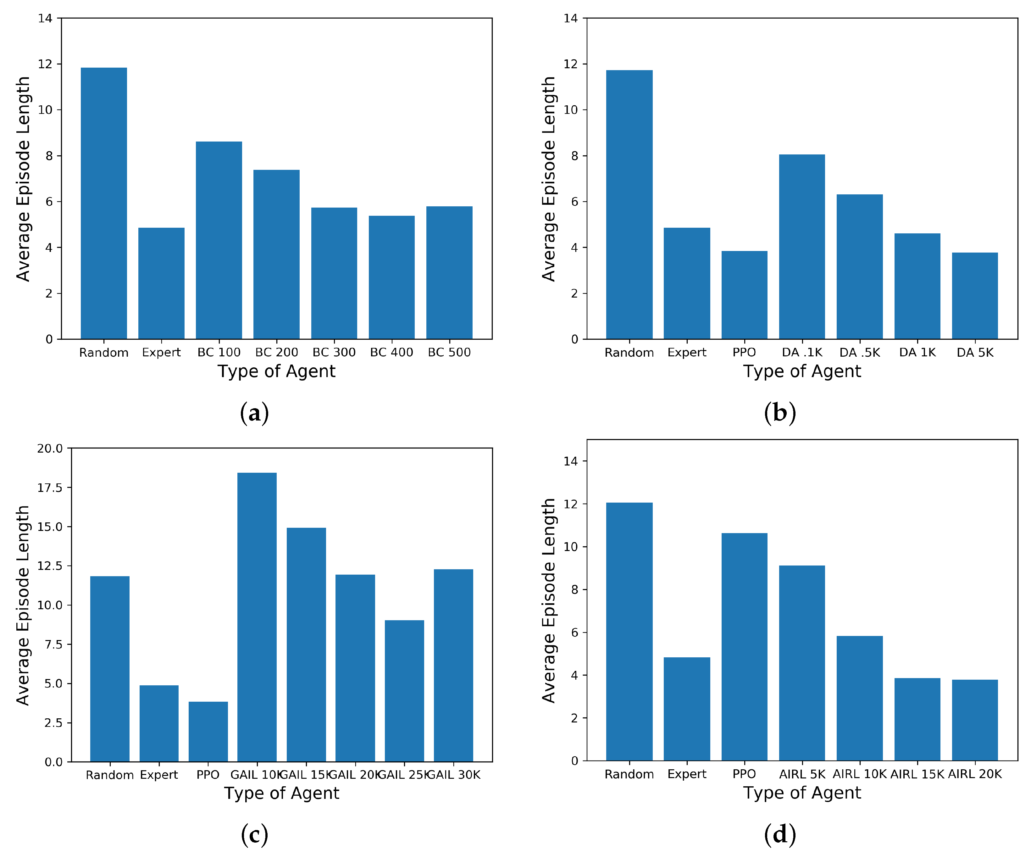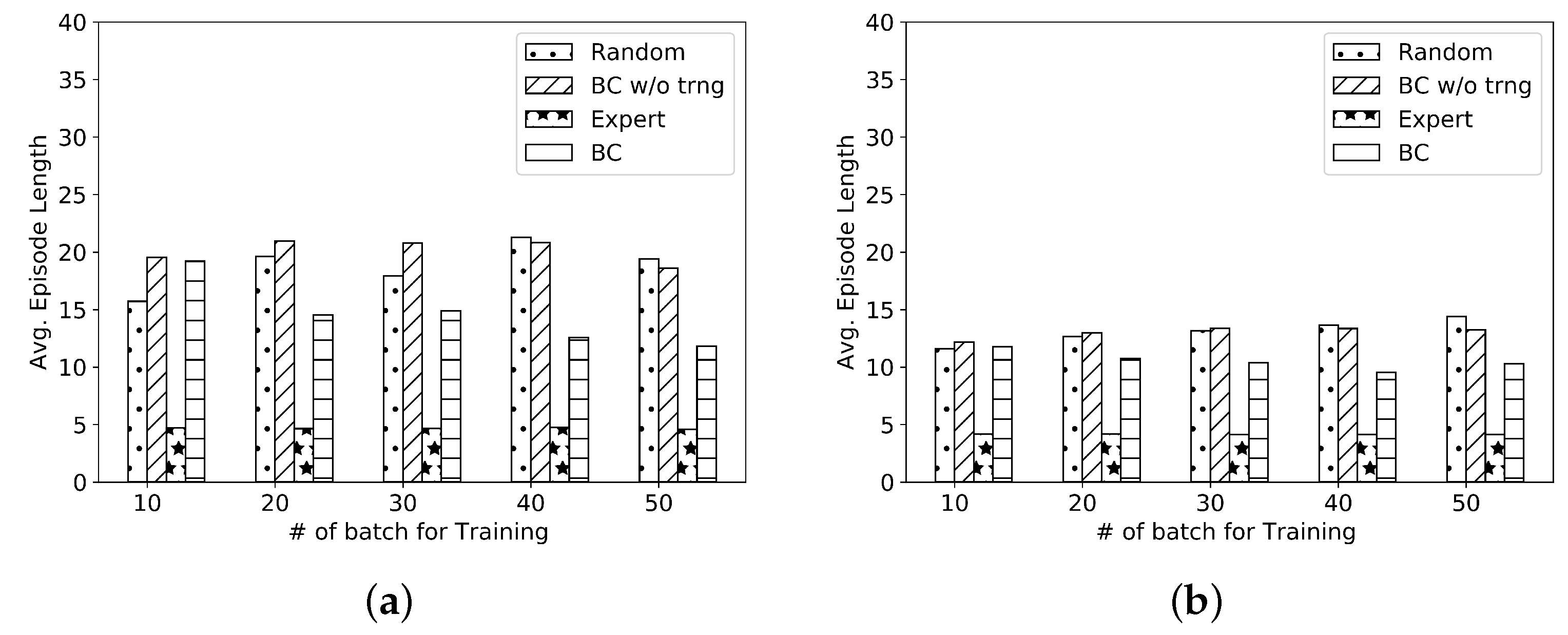Based on the different line outages considered in this work, the sequence of switching is obtained, and it can be observed from Figure 5a that the expert’s episode length is almost one-third of the random agent.

6. Results and Analysis

This study considers a IEEE 123-bus system with eight sectionalizing switches used for network reconfiguration to restore critical loads after line-outages. The IEEE 123-bus test system is a widely used benchmark in power systems research. It represents a realistic medium-voltage distribution network with 123 buses (nodes) and includes a mix of load, generation, and distribution lines. This provides a detailed but manageable network size for testing RL algorithms, which often require simulations of large-scale systems. While the IEEE 123-bus system is not as large as some real-world distribution grids, it is large enough to capture the complexity and diversity seen in power system such as load variations, distributed generation sources, and different operating conditions and contingencies.

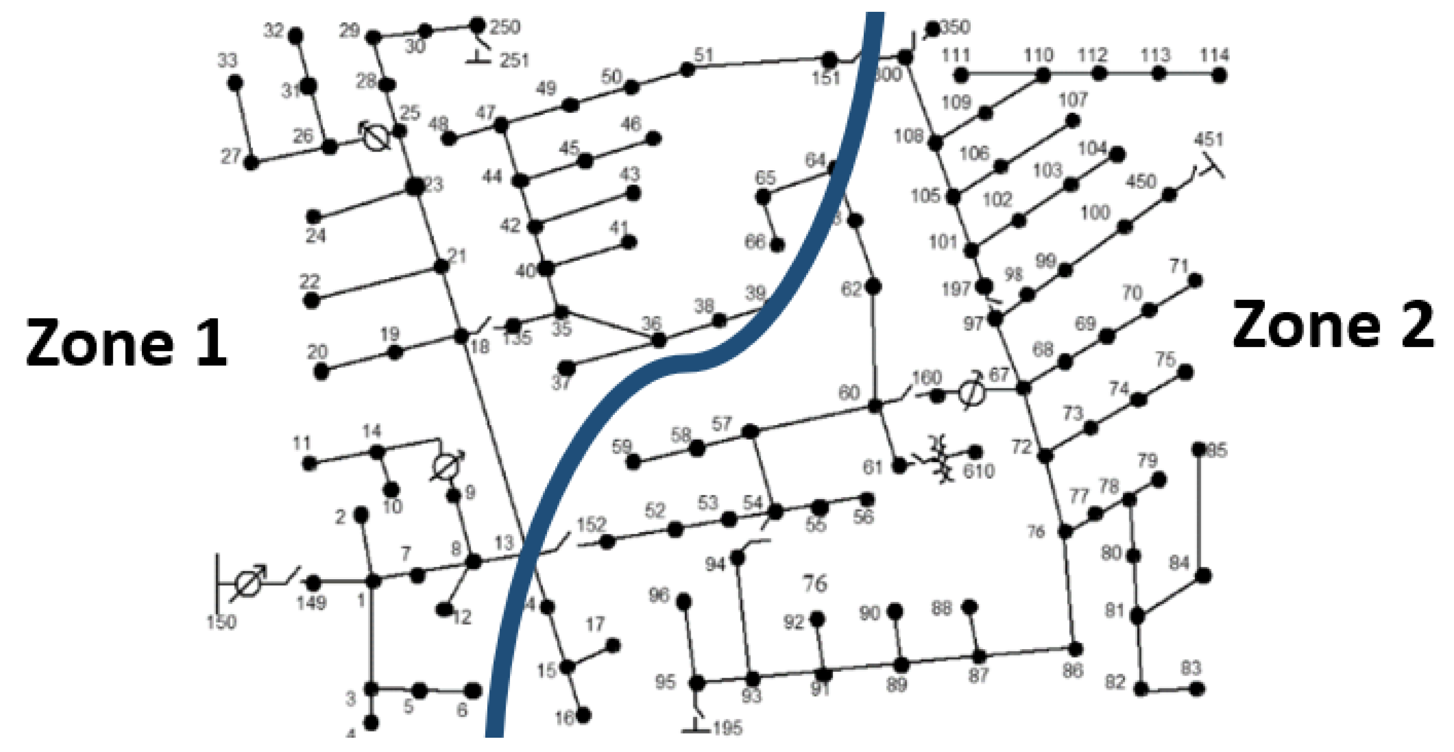
The communication network of this feeder system is developed based on segregation of the distribution feeder network into two zones (Figure 6), with each zone consisting of a DC, which forwards the collected real-time data from the smart meters and field devices from the respective zones to the DA. In a typical small- to medium-sized neighborhood, a distribution feeder could have anywhere from 50 to 100 nodes. Given 123 nodes in the IEEE 123-bus system, two zones representing two Neighborhood Area Network (NANs) are considered. The experiments in this work focus on learning resilience metrics in three MDP problems: (a) rerouting for the successful transmission of packets, (b) network reconfiguration for critical load restoration, and (c) a cyber–physical scenario for critical load restoration through both rerouting and network reconfiguration. We aim to answer these two questions:

• Can we reduce the episode lengths for variable-length MDPs by training a policy using expert demonstrations compared to forward RL techniques?
• Is the approach of imitation learning through an adaptive resilience metrics learning better compared to other forward RL techniques?

The hyper-parameters considered for the four approaches: (a) behavioral cloning, (b) DAgger, (c) GAIL and (d) AIRL are presented in

Table 1. Hyperparameters considered for training using behavioral cloning.

MDP Model	Hyperparameters
	Batch Size	# of Batches	Expert Rollouts
MDP 1	32	[10, 20, 30, 40, 50]	600
MDP 2	32	[100, 200, 300, 400, 500]	500
MDP 3	32	[10, 20, 30, 40, 50]	600

,

Table 2. Hyperparameters considered for training using DAgger.

MDP Model	Hyperparameters
	Initial Policy  $\mathit{\pi }$, Train Steps	Train Steps	Expert Rollouts
MDP 1	20,000	[1K, 2K, 3K, 4K, 5K]	2500
MDP 2	2000	[5K, 10K, 15K, 20K, 25K]	1000
MDP 3	20,000	[100, …, 1000]	2500

,

Table 3. Hyperparameters considered for training using GAIL.

MDP Model	Hyperparameters
	Initial Policy  $\mathit{\pi }$, Train Steps	Train Steps	Expert Rollouts
MDP 1	20,000	[30K, 75K, 150K, 300K]	500
MDP 2	2000	[10K, 15K, 20K, 25K, 30K]	2000
MDP 3	20,000	[30K, 75K, 150K, 300K]	500

and

Table 4. Hyperparameters considered for training using AIRL.

MDP Model	Hyperparameters
	Initial Policy  $\mathit{\pi }$, Train Steps	Train Steps	Expert Rollouts
MDP 1	20,000	[30K, 75K, 150K, 300K]	500
MDP 2	20,000	[5K, 10K, 15K, 20K]	1000
MDP 3	20,000	[30K, 75K, 150K, 300K]	500

, respectively. Additionally, the impact of the entropy regularizer on the training of the AIRL agent is also considered in Section 6.2.5.

6.1. Cyber-Side Resilience Metric Learning

Various imitation learning techniques are considered for evaluation: behavioral cloning, DAgger, GAIL, and AIRL. Techniques such as DAgger interact with the environment during training, whereas GAIL explores randomly to determine which action brings a policy occupancy measure as close to the expert’s policy ${\rho }_E$. These techniques’ performance will be evaluated for solving the re-routing problem on the basis of average number of episodes to reach the targeted goal, i.e., depending on the fixed number of packets successfully received at the destination node while there are cyber attacks on the routers.

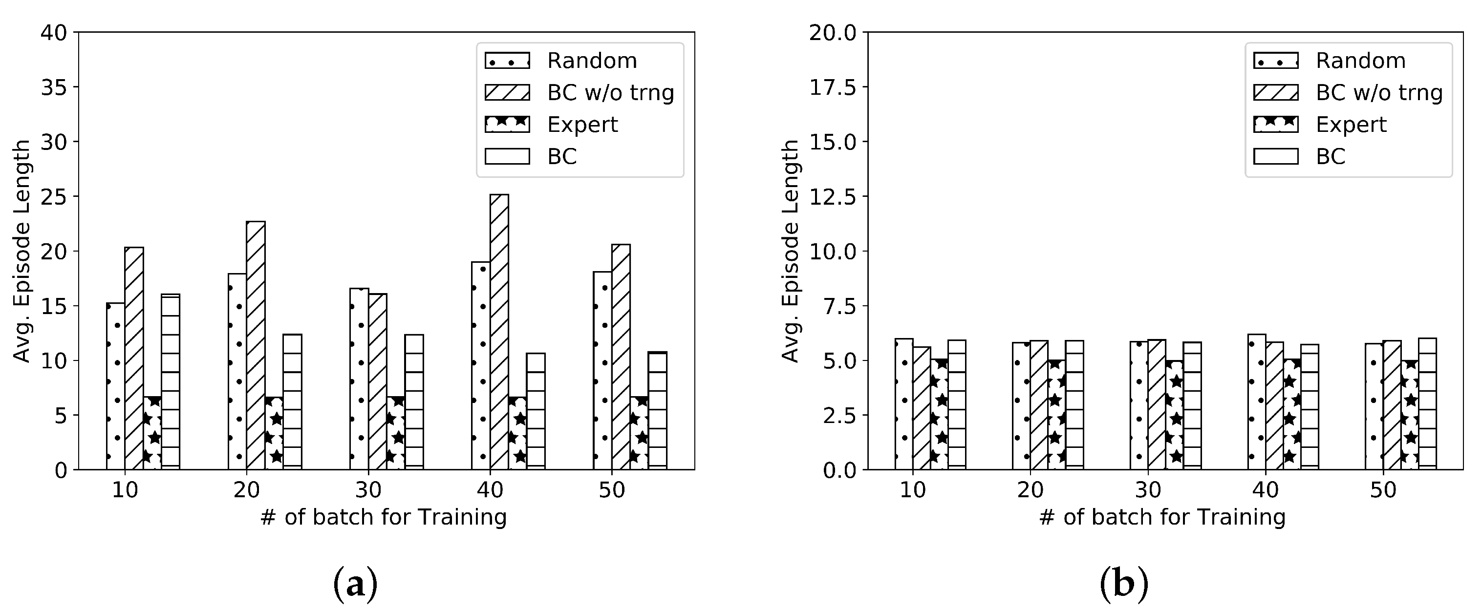
6.1.1. Evaluation of Behavioral Cloning

For both the networks, $N_g$ packets are set to five for both the DCs. Figure 7a,b present the results of the average episode length obtained using behavioral cloning-based imitation learning for the two networks under study. The average episode length with the trained $BC$ model is decreased more than 40% compared to the random or an untrained BC model $BCw/otrng$ for the $N_6$ network. Lower average episode length for the $N_8$ network represents that it is easier to train compared to the $N_6$ network.

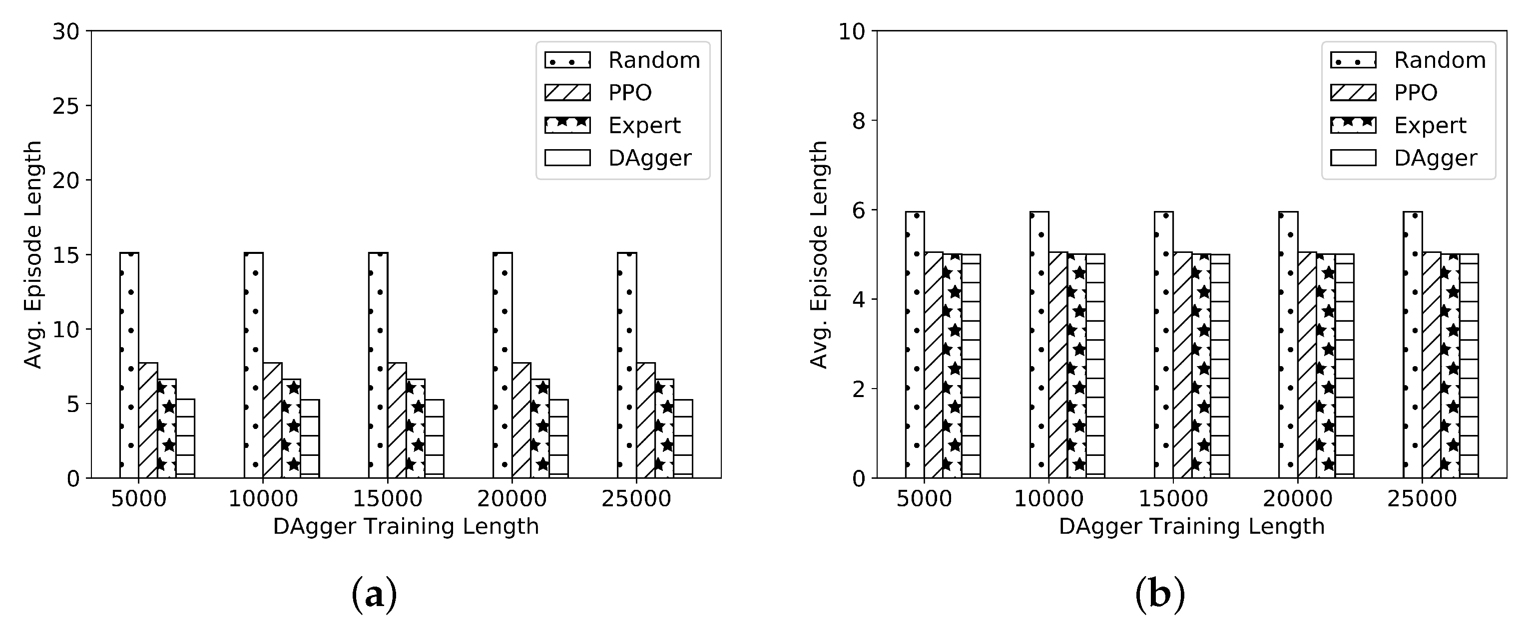
6.1.2. Evaluation of the DAgger Approach

Unlike behavioral cloning, which relies solely on the expert’s demonstrations for training, DAgger incorporates a feedback loop for learning. The agent actively participates in data collection by executing its policy and receiving corrective feedback from an expert or a more accurate policy. In our case, a PPO trained policy is considered for the corrective feedback steps. Figure 8a,b present the results for DAgger-based imitation learning for the two networks. The average episode length using DAgger is reduced compared to the PPO-based technique as well as the $BC$ technique. Though in this work, multi-modal expert demonstration is not considered, DAgger can handle multi-modal expert demonstrations more effectively than behavioral cloning.

6.1.3. Evaluation of GAIL

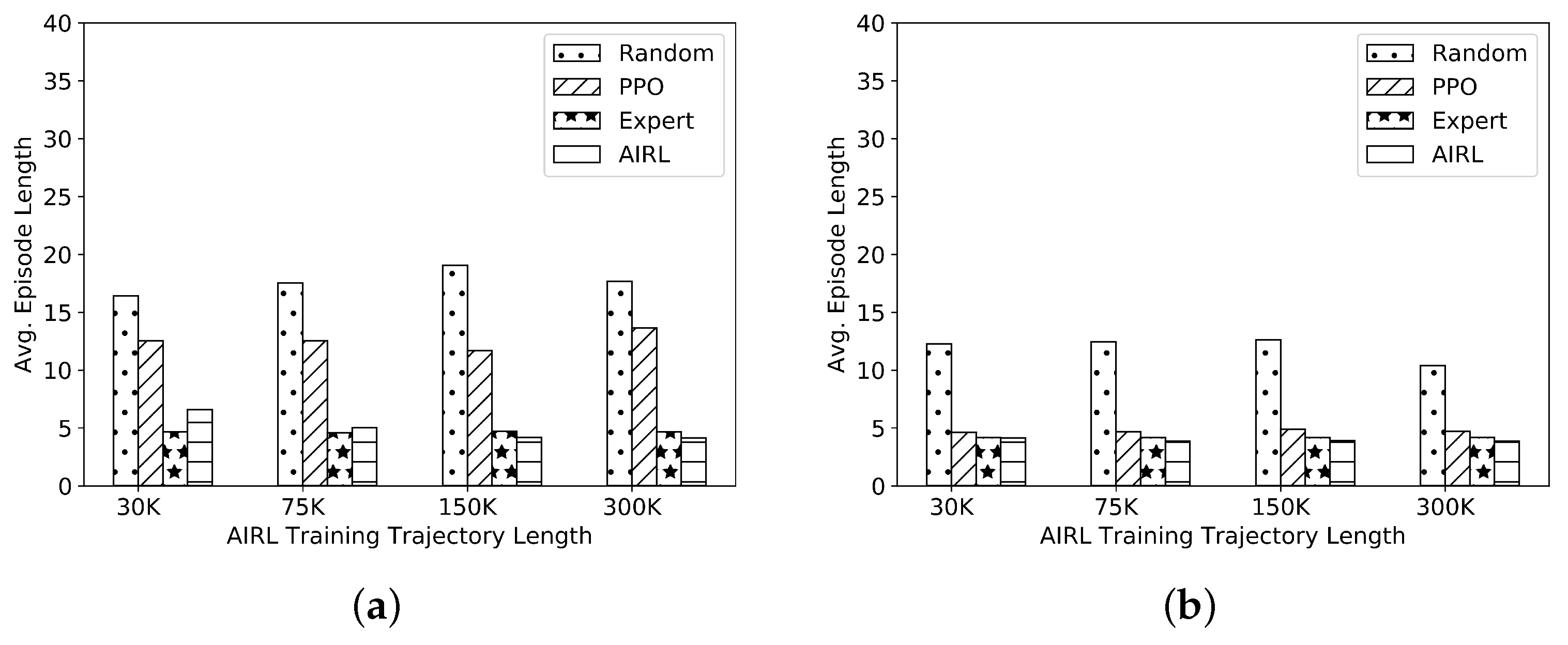
Figure 9a,b present the results using GAIL for the two communication networks of the distribution feeders. Compared to the DAgger and behavioral cloning technique, the GAIL method performance is improved. But to obtain improved performance, the GAIL trainer utilizes 300K time steps. For the $N_8$ network, it needs at least 150K transition samples to train an accurate agent.

6.1.4. Evaluation of the AIRL Method

AIRL can guide the agent’s exploration more efficiently towards behaviors that align with the expert’s demonstrations. In contrast, the policy learning process of GAIL can be more sample intensive since it relies solely on the discriminator’s feedback without direct guidance from a learned reward function. Figure 10a,b present the results of the average episode length obtained using AIRL for the two communication networks under study. A PPO generator network is considered for the GANs. The reward or the discriminator network consists of two hidden layers of 32 neurons each, and the input layer dimension depends on the observation and action space. Results from Figure 10b show that with the use of AIRL, the best performance is obtained with 30K transition trajectories for training as compared to GAIL in Figure 9b, which needs almost 300K samples. Hence, the performance of AIRL is better than GAIL in terms of both accuracy and sample efficiency.

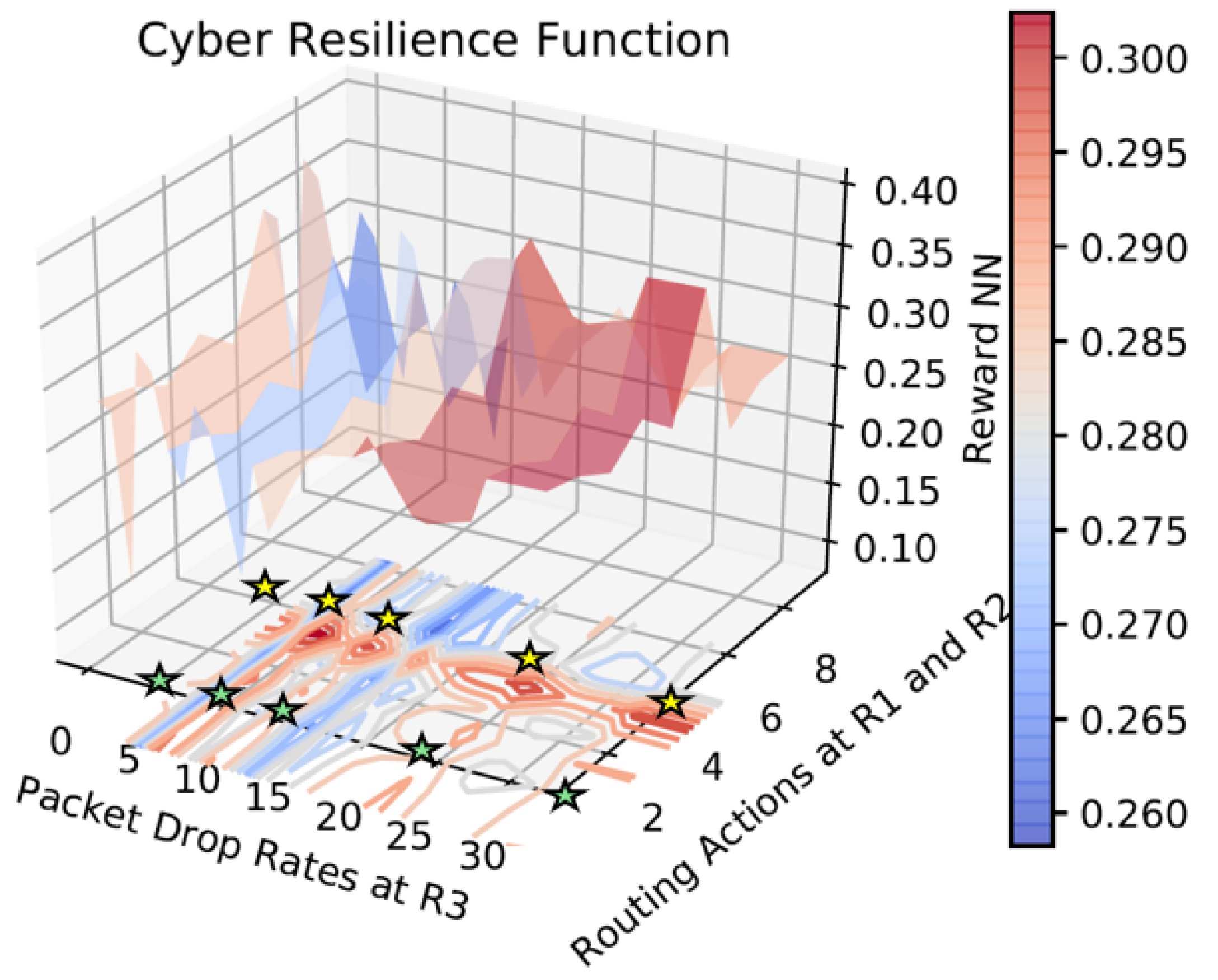
Figure 11 shows the resilience metric, i.e., the reward function learned as the function of the state and action, where the state is of the router $R_3$ and its packet drop rate, and the action is the routing options for router $R_1$ and $R_2$ encoded as per

Table 5. Encoded action for rerouting.

${\mathit{R}}_1$, ${\mathit{R}}_2$	Encoded Action	Description
0, 0	0	$R_1\to R_4$, $R_2\to R_3$
1, 0	1	$R_1\to R_6$, $R_2\to R_3$
2, 0	2	$R_1\to R_3$, $R_2\to R_3$
0, 1	3	$R_1\to R_4$, $R_2\to R_7$
1, 1	4	$R_1\to R_6$, $R_2\to R_7$
2, 1	5	$R_1\to R_3$, $R_2\to R_7$
0, 2	6	$R_1\to R_4$, $R_2\to R_5$
1, 2	7	$R_1\to R_6$, $R_2\to R_5$
2, 2	8	$R_1\to R_3$, $R_2\to R_5$

. For the $N_8$ network (Figure 2), $R_1$ and $R_2$ have three interfaces each, making a total of nine possible actions. Routing action zero represents $R_1$ selecting its first interface $R_4$, and $R_2$ selecting its first interface $R_3$. From the learned function, it can be observed that as the packet drop rate at $R_3$ increases, and the encoded action is preferably more than four, making $R_2$ select either $R_7$ or $R_5$. Since the visualization of the reward function with all the observation and action space is harder in three dimensions, only one observation and two actions are visualized in Figure 11. Moreover, the action space in this problem is multi-discrete, and it is not possible to obtain a monotonically increasing or decreasing reward function. Hence, the obtained reward function is a non-convex function. In order to obtain a smooth convex reward function, one needs to train neural networks that learn a convex function using procedures prescribed in the literature [36] and also make alteration in the environment, which is not possible for the rerouting problem since the notion of interfaces in the router cannot be made continuous.

6.2. Physical-Side Resilience Metric Learning

For the power system resilience metric learning, we consider the variable-length episode-based network reconfiguration problem.

6.2.1. Evaluation of the Behavioral Cloning Approach

Figure 5a shows the comparison of training the behavior cloning-based agent by varying the number of batches loaded from the data set before ending the training. It can be observed that the average episode length decreases with an increase in the number of batches, but it never stabilizes, and it is relatively higher than the expert.

6.2.2. Evaluation of the DAgger Method

Figure 5b shows the comparison of training the DAgger-based agent by varying the training samples, i.e., total number of time steps. It can be observed that the average episode length decreases with increases in the data samples. For 5000 data samples, the average episode length is less than the expert. Though this assists in improving the performance compared to behavior cloning, this method is computationally expensive because the training is sequentially performed in a loop (refer to Algorithm 3).

6.2.3. Evaluation of the GAIL Method

Figure 5c shows the comparison of training the GAIL-based agent by varying the training samples, i.e., total number of time steps. With more training samples, the episode length to reach the goal reduces, but the performance is not better than the PPO method.

6.2.4. Evaluation of the AIRL Method

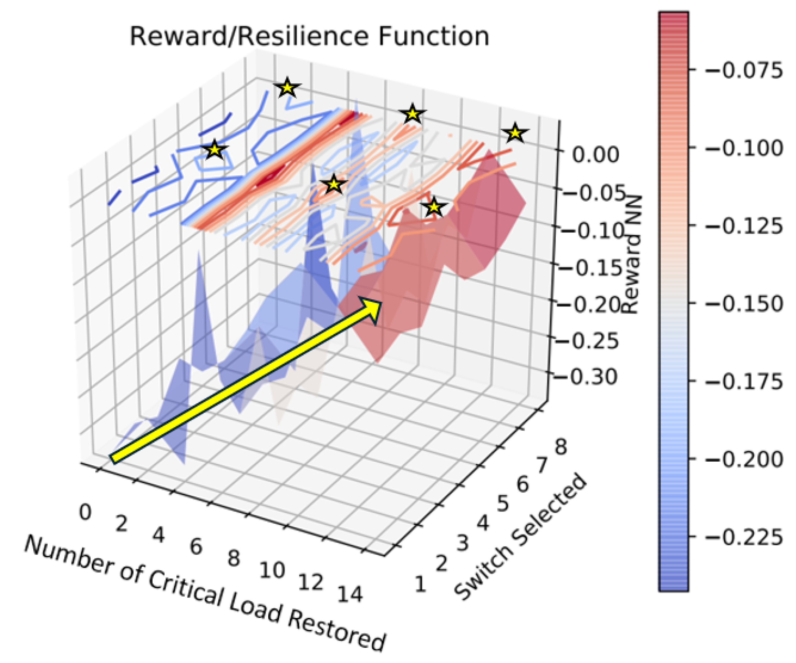
Figure 5d shows the comparison of training the AIRL-based agent by varying the training samples, i.e., total number of time steps. Figure 12 shows the resilience metric, or the reward function learned as the function of the state and action, where the state is indicated through the number of critical loads restored, and the action is indicated through the sectionalizing switch selected in the IEEE 123-bus case. (There are nine switches in the model, of which the main switch connected to the substation transformer is not selected for the control action; hence, the Switch Selected axis is visible until eight.) From the learned function, it can be observed that the reward function is increased with the number of critical loads restored. Though there is a monotonic rise in the reward with reference to the observation space, i.e., number of critical load restored, but we cannot obtain a continuous function with reference to the action i.e., Switch Selected axis. Each of the switches has a different impact on the voltage of the critical load depending on its location on the feeder model, and hence we cannot assume that switches numbered N restore the voltage better than the switches numbered $\ge N$ to observe a monotonic drop in reward, or Switch N restores the voltage better than Switch $\le N$ to observe a monotonic rise in reward.

6.2.5. Impact of Entropy Regularization Coefficient on Training

This section discusses the impact of entropy regularization on the training of the discriminator. The discriminator can easily overfit to distinguish expert vs. generated samples, especially when the policy is weak early on. Since there is subtraction of the entropy term, a low-entropy term will prevent the discriminator from becoming overconfident. Hence, if there are limited expert data, the discriminator might memorize the expert samples; hence, a lower-entropy regularization coefficient is better. We will take a scenario with 500 and 2000 expert trajectories and evaluate what is an ideal entropy coefficient. It can be observed from the accuracy plot of the discriminator training that the scenario where the agent is trained with 500 expert trajectories, an entropy coefficient $\lambda$ (refer to line 15 of Algorithm 4) of 0.01 is preferred (Figure 13a), while for the case where the agent is trained with 2000 expert trajectories, a $\lambda$ of 0.1 is preferred (Figure 13b). But in all the scenarios where the entropy coefficient is too high, it will have slower convergence on the policy, and hence it is better to schedule the entropy coefficient in the training process by starting with a higher value and gradually reducing it.

6.3. Cyber–Physical Resilience Metric Learning

6.3.1. Evaluation of Behavioral Cloning

For both the networks, $N_g$ packets are set to five for both the DCs. Figure 14a,b present the results of the average episode length obtained using behavioral cloning-based imitation learning for the two networks under study.

6.3.2. Evaluation of the DAgger Approach

Figure 15a,b present the results for DAgger-based imitation learning for the two networks. The average episode length using DAgger is reduced compared to the PPO-based technique as well as the $BC$ technique.

6.3.3. Evaluation of GAIL

Figure 16a,b present the results using GAIL for the two respective communication networks of the distribution feeders. The GAIL performance deteriorated drastically in the cyber–physical problem compared to the individual problems, hence proving its ineffectiveness against a complex task. Moreover, GAIL would face scalability issue since the training is sample inefficient.

6.3.4. Evaluation of the AIRL Method

Figure 17a,b present the results of the average episode length obtained using AIRL for the two different networks under study. The same generator and discriminator models were considered as used for the cyber-only rerouting problem. For the cyber–physical control problem, the performance of AIRL is much better than GAIL in terms of the average episode length to restore all critical loads through switching and rerouting. Training AIRL with 150K transition samples, the performance is better than the expert. AIRL exhibits greater robustness to changes in the environment or the usage of multiple diverse environment compared to GAIL. By directly learning the reward function, the agent’s behavior is guided by the underlying intent of the expert demonstrations, which leads to more consistent performance across different environments. Figure 18 shows the cyber–physical resilience metric, i.e., the reward function learned as the function of the cyber and physical action, where the physical action is one of the sectionalizing switch in the IEEE 123 bus selected, and the cyber action is the routing option for router $R_1$ and $R_2$ encoded as per Table 5.

7. Challenges of Proposed Approach

Given that the resilience of a system is scenario- and time dependent, it is crucial to incorporate an adaptive reward model instead of a fixed reward for the MDPs. Hence, in this work, instead of leveraging forward RL for training agents on a complete MDP, IRL is proposed for learning the reward model for an incomplete MDP with the reward function undefined. The challenges in this approach are two-fold: (a) obtaining expert demonstrations, and (b) fidelity to computation trade-offs. To obtain expert demonstrations, we currently implemented heuristic and established optimization methods. In a utility, the expert demonstrations can be incorporated by obtaining historical control/measurements, or directly from operators.

The fidelity of the experiments depends on the modeling accuracy of the SimPy-based cyber environment. There are challenges associated with learning cyber–physical combined reward functions because of two reasons: (a) It requires the generation of enough high-fidelity expert demonstrations. In these experiments, heuristic and spanning tree-based approaches are considered for generating the expert trajectories, which might not be optimal while considering the combined cyber–physical environment. (b) The SimPy-based cyber environment considered is not as high fidelity in the sense of the packet drop rate and delay calculation compared to its counterparts, such as Mininet, CORE, or NS-3 emulators. Because the RL agents are data hungry to generate optimal policies, the lightweight environment is used in this case. Unlike the predefined resilience metric, the visualization of the reward neural network as a function of high-dimensional action and state pairs is one of the major challenges which can be tackled in future works, but currently the impact of each state and action variable in the reward/ resilience metric can be evaluated as shown in Figure 11, Figure 12 and Figure 18. In the future, this approach will be tested for a bigger utility-based feeder, and the computational cost associated with learning the metric will be evaluated.

8. Conclusions

This paper demonstrated a novel approach for adaptively learning the resilience metric and learning policy using imitation learning techniques for a combined power distribution system and its associated communication network for network restoration, optimal rerouting, and cyber–physical critical load restoration. For all these control problems, the $AIRL$ technique provided improved performance by reducing the average number of steps to reach the goal states, and it allowed us to train the reward neural network. This method can be incorporated into other cyber–physical control problems, such as volt-var control, automatic generation control, and automatic voltage regulation. Moreover, $AIRL$ is sample efficient in comparison to other approaches, making it effective for larger cyber–physical systems. In future work, we will be (a) evaluating multi-agent variant of AIRL for the cyber–physical RL problem; (b) scaling up to train for larger feeder cases, and extending to transmission system networks, and (c) exploring approaches to convexify and generate unique reward functions.

References

- Murino, G.; Armando, A.; Tacchella, A. Resilience of Cyber-Physical Systems: An Experimental Appraisal of Quantitative Measures. In Proceedings of the 2019 11th International Conference on Cyber Conflict, Tallinn, Estonia, 28 May–31 May 2019; Volume 900, pp. 1–19. [Google Scholar] [CrossRef]
- Bhusal, N.; Abdelmalak, M.; Kamruzzaman, M.; Benidris, M. Power System Resilience: Current Practices, Challenges, and Future Directions. IEEE Access 2020, 8, 18064–18086. [Google Scholar] [CrossRef]
- Bordeau, J.D.; Graubart, R.D.; McQuaid, R.M.; Woodill, J. Enabling Systems Engineers and Program Managers to Select the Most Useful Assessment Methods; The MITRE Corporation: McLean, VA, USA, 2018. [Google Scholar]
- Bordeau, D.J.; Graubart, R.D.; McQuaid, R.M.; Woodill, J. Cyber Resiliency Metrics and Scoring in Practice; The MITRE Corporation: McLean, VA, USA, 2018. [Google Scholar]
- Linkov, I.; Eisenberg, D.A.; Plourde, K.; Seager, T.P.; Allen, J.; Kott, A. Resilience metrics for cyber systems. Environ. Syst. Decis. 2013, 33, 471–476. [Google Scholar] [CrossRef]
- Tushar; Venkataramanan, V.; Srivastava, A.; Hahn, A. CP-TRAM: Cyber-Physical Transmission Resiliency Assessment Metric. IEEE Trans. Smart Grid 2020, 11, 5114–5123. [Google Scholar] [CrossRef]
- Venkataramanan, V.; Hahn, A.; Srivastava, A. CP-SAM: Cyber-Physical Security Assessment Metric for Monitoring Microgrid Resiliency. IEEE Trans. Smart Grid 2020, 11, 1055–1065. [Google Scholar] [CrossRef]
- Fonseca, C.M.; Klamroth, K.; Rudolph, G.; Wiecek, M.M. Scalability in Multiobjective Optimization (Dagstuhl Seminar 20031). Dagstuhl Rep. 2020, 10, 52–129. [Google Scholar] [CrossRef]
- Huang, Y.; Huang, L.; Zhu, Q. Reinforcement Learning for Feedback-Enabled Cyber Resilience. Annu. Rev. Control 2022, 53, 273–295. [Google Scholar] [CrossRef]
- Kott, A.; Linkov, I. To Improve Cyber Resilience, Measure It. Computer 2021, 54, 80–85. [Google Scholar] [CrossRef]
- Panteli, M.; Mancarella, P.; Trakas, D.N.; Kyriakides, E.; Hatziargyriou, N.D. Metrics and Quantification of Operational and Infrastructure Resilience in Power Systems. IEEE Trans. Power Syst. 2017, 32, 4732–4742. [Google Scholar] [CrossRef]
- Hussain, A.; Bui, V.H.; Kim, H.M. Microgrids as a resilience resource and strategies used by microgrids for enhancing resilience. Appl. Energy 2019, 240, 56–72. [Google Scholar] [CrossRef]
- Fesagandis, H.S.; Jalali, M.; Zare, K.; Abapour, M.; Karimipour, H. Resilient Scheduling of Networked Microgrids Against Real-Time Failures. IEEE Access 2021, 9, 21443–21456. [Google Scholar] [CrossRef]
- Umunnakwe, A.; Huang, H.; Oikonomou, K.; Davis, K. Quantitative analysis of power systems resilience: Standardization, categorizations, and challenges. Renew. Sustain. Energy Rev. 2021, 149, 111252. [Google Scholar] [CrossRef]
- Zhou, Y.; Panteli, M.; Wang, B.; Mancarella, P. Quantifying the System-Level Resilience of Thermal Power Generation to Extreme Temperatures and Water Scarcity. IEEE Syst. J. 2020, 14, 749–759. [Google Scholar] [CrossRef]
- Memarzadeh, M.; Moura, S.; Horvath, A. Optimizing dynamics of integrated food–energy–water systems under the risk of climate change. Environ. Res. Lett. 2019, 14, 074010. [Google Scholar] [CrossRef]
- Hossain-McKenzie, S.; Lai, C.; Chavez, A.; Vugrin, E. Performance-Based Cyber Resilience Metrics: An Applied Demonstration Toward Moving Target Defense. In Proceedings of the IECON 2018—44th Annual Conference of the IEEE Industrial Electronics Society, Washington, DC, USA, 21–23 October 2018; pp. 766–773. [Google Scholar] [CrossRef]
- Friedberg, I.; McLaughlin, K.; Smith, P.; Wurzenberger, M. Towards a Resilience Metric Framework for Cyber-Physical Systems. In Proceedings of the 4th International Symposium for ICS & SCADA Cyber Security Research 2016, Swindon, UK, 23–25 August 2016; ICS-CSR’16. pp. 1–4. [Google Scholar] [CrossRef]
- Yin, L.; Zhang, C.; Wang, Y.; Gao, F.; Yu, J.; Cheng, L. Emotional Deep Learning Programming Controller for Automatic Voltage Control of Power Systems. IEEE Access 2021, 9, 31880–31891. [Google Scholar] [CrossRef]
- Zhou, Y.; Zhang, B.; Xu, C.; Lan, T.; Diao, R.; Shi, D.; Wang, Z.; Lee, W.J. A Data-driven Method for Fast AC Optimal Power Flow Solutions via Deep Reinforcement Learning. J. Mod. Power Syst. Clean Energy 2020, 8, 1128–1139. [Google Scholar] [CrossRef]
- Chen, X.; Li, Y.; Shimada, J.; Li, N. Online Learning and Distributed Control for Residential Demand Response. IEEE Trans. Smart Grid 2021, 12, 4843–4853. [Google Scholar] [CrossRef]
- Utkarsh, K.; Ding, F. Self-Organizing Map-Based Resilience Quantification and Resilient Control of Distribution Systems Under Extreme Events. IEEE Trans. Smart Grid 2022, 13, 1923–1937. [Google Scholar] [CrossRef]
- Chen, J.; Hu, S.; Zheng, H.; Xing, C.; Zhang, G. GAIL-PT: An intelligent penetration testing framework with generative adversarial imitation learning. Comput. Secur. 2023, 126, 103055. [Google Scholar] [CrossRef]
- Zennaro, F.M.; Erdődi, L. Modelling penetration testing with reinforcement learning using capture-the-flag challenges: Trade-offs between model-free learning and a priori knowledge. IET Inf. Secur. 2023, 17, 441–457. [Google Scholar] [CrossRef]
- Ye, Y.; Wang, H.; Xu, B.; Zhang, J. An imitation learning-based energy management strategy for electric vehicles considering battery aging. Energy 2023, 283, 128537. [Google Scholar] [CrossRef]
- Xu, S.; Zhu, J.; Li, B.; Yu, L.; Zhu, X.; Jia, H.; Chung, C.Y.; Booth, C.D.; Terzija, V. Real-time power system dispatch scheme using grid expert strategy-based imitation learning. Int. J. Electr. Power Energy Syst. 2024, 161, 110148. [Google Scholar] [CrossRef]
- Sahu, A.; Venkataramanan, V.; Macwan, R. Reinforcement Learning Environment for Cyber-Resilient Power Distribution System. IEEE Access 2023, 11, 127216–127228. [Google Scholar] [CrossRef]
- Elnaggar, M.; Bezzo, N. An IRL Approach for Cyber-Physical Attack Intention Prediction and Recovery. In Proceedings of the 2018 Annual American Control Conference (ACC), Milwaukee, WI, USA, 27–29 June 2018; pp. 222–227. [Google Scholar] [CrossRef]
- Adams, S.; Cody, T.; Beling, P. A survey of inverse reinforcement learning. Artif. Intell. Rev. 2022, 55, 4307–4346. [Google Scholar] [CrossRef]
- Ramachandran, D.; Amir, E. Bayesian Inverse Reinforcement Learning. In Proceedings of the 20th International Joint Conference on Artificial Intelligence, San Francisco, CA, USA, 25–27 January 2007; IJCAI’07. pp. 2586–2591. [Google Scholar]
- Ross, S.; Gordon, G.J.; Bagnell, J.A. A Reduction of Imitation Learning and Structured Prediction to No-Regret Online Learning. arXiv 2010. [Google Scholar] [CrossRef]
- Ho, J.; Ermon, S. Generative Adversarial Imitation Learning. arXiv 2016. [Google Scholar] [CrossRef]
- Fu, J.; Luo, K.; Levine, S. Learning Robust Rewards with Adversarial Inverse Reinforcement Learning. arXiv 2017. [Google Scholar] [CrossRef]
- Sahu, A. ARM-IRL: Adaptive Resilience Metric Quantification Using Inverse Reinforcement Learning. arXiv 2024, arXiv:2501.12362. [Google Scholar] [CrossRef]
- Li, J.; Ma, X.Y.; Liu, C.C.; Schneider, K.P. Distribution System Restoration with Microgrids Using Spanning Tree Search. IEEE Trans. Power Syst. 2014, 29, 3021–3029. [Google Scholar] [CrossRef]
- Bengio, Y.; Roux, N.; Vincent, P.; Delalleau, O.; Marcotte, P. Convex Neural Networks. In Advances in Neural Information Processing Systems; Weiss, Y., Schölkopf, B., Platt, J., Eds.; MIT Press: Cambridge, MA, USA, 2005. [Google Scholar]
Figure 1.
Communication network, , where all the six routers are controllable and the DoS attack is performed at any of the routers = .
Figure 2.
Communication network, , where three out of eight routers are controllable.
Figure 3.
GAN architecture for policy and reward learning.
Figure 4.
Overall architecture of ARM-IRL.
Figure 5.
Comparison of (a) the behavior cloning technique with random and other behavioral cloning agents with training under different batch sizes used for training, (b) DAgger technique with random PPO agents with training under different transition samples, (c) GAIL, and (d) AIRL technique with random PPO agents with training under different transition samples.
Figure 6.
IEEE 123 test system segregated to two zones.
Figure 7.
Evaluation of the behavioral cloning for cyber network of (a) and (b) with two unique action spaces.
Figure 8.
Evaluation of the DAgger algorithm for the cyber network of (a) and (b) with two unique action spaces.
Figure 9.
Evaluation of the GAIL method for the cyber network of (a) and (b) with two unique action spaces.
Figure 10.
Evaluation of the AIRL method for the cyber network of (a) and (b) with two unique action spaces.
Figure 11.
Reward as a function of the packet drop rate at the router R3 and the action taken at router R1 and R2. The highest peaks in the reward, highlighted in yellow, are when the encoded action 6 (R1 select its interface to R4, R2 select its interface to R5) is selected from