Classification of Exoplanetary Light Curves Using Artificial Intelligence

Abstract

In this article, we propose a robust star classification methodology leveraging light curves collected from 15 datasets within the Kepler field in the visible optical spectrum. By employing a Bagging neural network ensemble approach, specifically an Bagging-Performance Approach Neural Network (BAPANN), which integrates three supervised neural network architectures, we successfully classified 760 samples of curves which represent 9 type of stars. Our method demonstrated a high classification accuracy of up to 97% using light curve datasets containing 13, 20, 50, 150, and 450 points per star. The BAPANN achieved a minimum error rate of 0.1559 and exhibited efficient learning, requiring an average of 29 epochs. Additionally, nine types of stellar variability were classified through 45 conducted tests, taking into account error margins of 0, 5, and 10 for the light curve samples. These results highlight the BAPANN model’s robustness against uncertainty and ability to converge quickly in terms of iterations needed for learning, training, and validation.

1. Introduction

The classification of the elements of the universe is crucial for creating accurate physical models for astrophysicists. However, the enormous amount of data observations carried out worldwide becomes overwhelming and intractable, necessitating the automation of data analysis through powerful and fast methods, such as artificial intelligence algorithms. Fortunately, artificial intelligence offers methods and approaches that can be effectively utilized to support this heavy task. Specifically, applications to identify or classify light curves based on their stellar variability in astrophysics have shown promising results. Some studies have achieved accuracy percentages close to 90% using light curves with about 2000 points, employing Fourier transform techniques, and, in some cases, using up to 7000 parametric statistics as input for the identification of stellar variability. These works, detailed in

Table 1. In the 1st and 2nd columns, the references and titles of the works are displayed. The 3rd column presents the number of characteristics each work utilizes, including the type of data (whether a light curve or statistical data), the number of points on the curve, and the number of classes the respective authors consider. The 4th column specifies the method used for either characterization or classification. The 5th column lists the accuracy percentage obtained by the authors and the number of stars included in their respective observation collections.

Reference	Title	Features	AI Method	Stars Number or %’s
Debosscher et al., (2007) [1]	Automated supervised classification of variable stars	28 statistics, of the TFD of the light curve, 35 categories and 14 categories	MGaussianM Mehalanobis BNC, ANNC SVM	60,000 stars BNC: 66% RNPB: 70% MSV: 50% MMG: 92%
Olmedo et al., (2015) [2]	Deep GALEX UV survey of the, Kepler Field	28 attributes	NUV	596,556 stars
Bass & Borne (2016) [3]	Supervised ensemble classification of Kepler variable stars	165 attributes of the light curve. 14 y 8 categories,	TFD-SAX SMOTE BN RFGC	150,000 stars BN: 64%
Olmedo et al., (2017) [4]	Ultraviolet variable sources in the Kepler field	10 attributes	NUV	6,818,181 stars
Audenaert et al., (2021) [5]	TESS Data for Asteroseismology (TDA) Stellar Variability Classification Pipeline: Setup and Application to the Kepler Q9 Data	26 statistics, 30 pointsof the light curve, 289 points of the TFD	SHORTING HAT GBGC Metodos no Supervised Meta assembly	167,243 stars Meta: 94.9%
Barbara et al., (2022) [6]	Light curves Classification for Kepler stars A and F by automatic learning based on features	7000 statistics, 2000 points of the light curve of the TFD, 7 groups	Library hctsa de Matlab	from 80.8–90% 1319 stars
Our work	Variability studies UV of stars with planets in the Kepler field by artificial intelligence codes	17 statistics, 50 points of the light curve 9 groups	BAPANN	760 stars 97.8%

, highlight the classification contributions achieved by various authors.

Multi-wavelength observations are essential to understanding the nature and evolution of astrophysical objects and phenomena. This emphasizes the importance of automatic classification through artificial intelligence and the need to catalog all stellar objects. Of particular relevance is that, for stars, observations in the ultraviolet range complement optical, infrared, and X-ray data, among others. The UV band explicitly allows the determination of atmospheric properties in solar-type stars, which impacts the conditions under which life can exist on exoplanets. In this work, we study the light curves in the visible spectrum from the Kepler mission data using artificial intelligence methods leading to variability detection. We consider nine classes of variability, including Eclipse, Constant, Aperiodic, Contact/Rotational type stars; Delta Scuti/Beta Cepheids; Flare, Gamma Doradus/SPB; RRLyrae/Cepheidas (noting that Beta Cepheids and Cepheids are distinctly different categories), and Solarlike stars. Our research is based on the collection of stars provided by Audenaert [5], excluding the Instrument class and including an additional class of Flare-type stars. As described below, we analyze 15 datasets with varying light curve points in the optical domain, aiming to further classify datasets in the ultraviolet domain. This work has the potential to be applied to other regions of the sky that lack optical light curves, such as the Kepler field, requiring reclassification of light curves in the NUV. This research aims to establish a standard that can be applied to other regions of the GALEX (Galaxy Evolution Explorer) sky, as referenced in the works of Miles [7], Olmedo [2], and Olmedo [4].

The paper is organized as follows: Section 1 provides the background information. Section 2 introduces the methodology for classifying Kepler light curves using artificial intelligence. Section 3 discusses the experiments conducted, followed by Section 4, which presents the results obtained. Finally, we conclude the paper with our final remarks in Section 5.

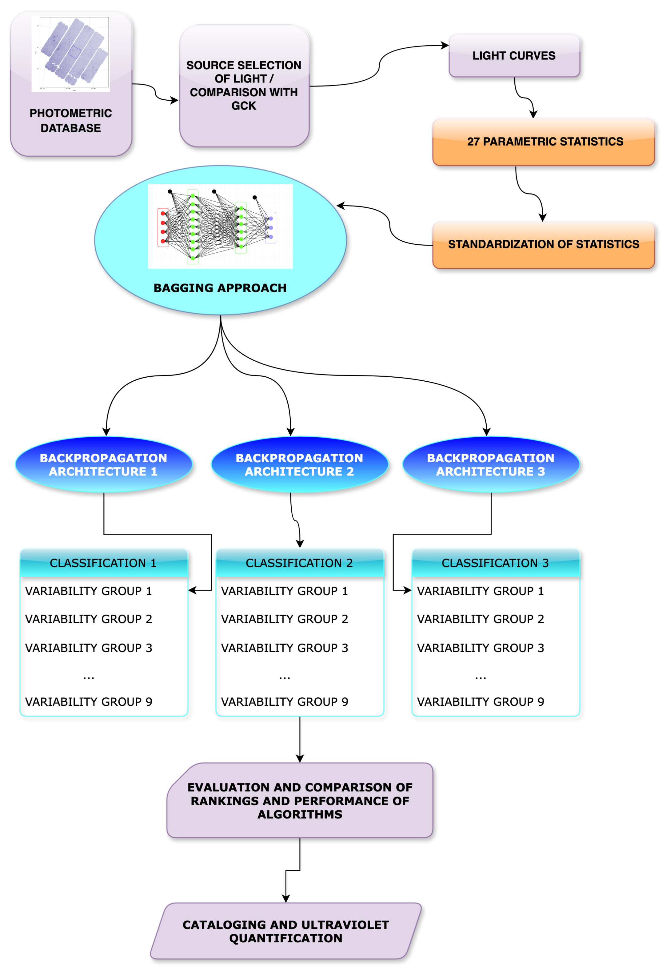
2. Methodology for Classifying Kepler Light Curves Using Artificial Intelligence

This research begins by familiarizing itself with the photometric database. The dataset comprises approximately 400,000 photometric data points of star sources obtained from the Galaxy Evolution Explorer (GALEX) space telescope [2,4]. In the near-ultraviolet spectrum (NUV; 2000–2800 Å), these light curves are derived from point sources observed by the Kepler telescope. Starting with the GALEX collection, the existence of each light source in the Kepler Input Catalog (KIC) is verified. If matches are found, the light curves that have undergone multiple observations are selected to form the input dataset, simulating the NUV sources while confirming their presence in the KIC. Our methodology uses the data to train the learning algorithms. Light curves of the selected light sources are generated, taking into account attributes such as exposure time and NUV flux. Samples are obtained with 400, 200, 100, 50, and 20 points of the light curve for each source from the GALEX collection. This stage aims to highlight the characteristics in the light curve points, providing a unique profile for each type of light curve to be classified. Twenty-seven parametric statistics are then calculated as a function of the NUV flux (simulated from the optical flux) based on the works of [5,7,8,9]. The neural network architectures used in this research require normalized data between 0 and 1 in real values for the input of the data sets. Therefore, the photometric data is normalized for each vector in the GALEX collection, as required by any neural network algorithm [10]. Each of the previously mentioned statistics is normalized to fit within the range of 0 to 1, ensuring compatibility with the neural network models. The backpropagation algorithm operates with real values and performs more effectively when the input data is normalized within this range. The project aims to classify the types of ultraviolet variability observed in stars or planetary systems into the following categories:

• Group 1 ECLIPSE: Eclipsing Binaries and Transit Events.
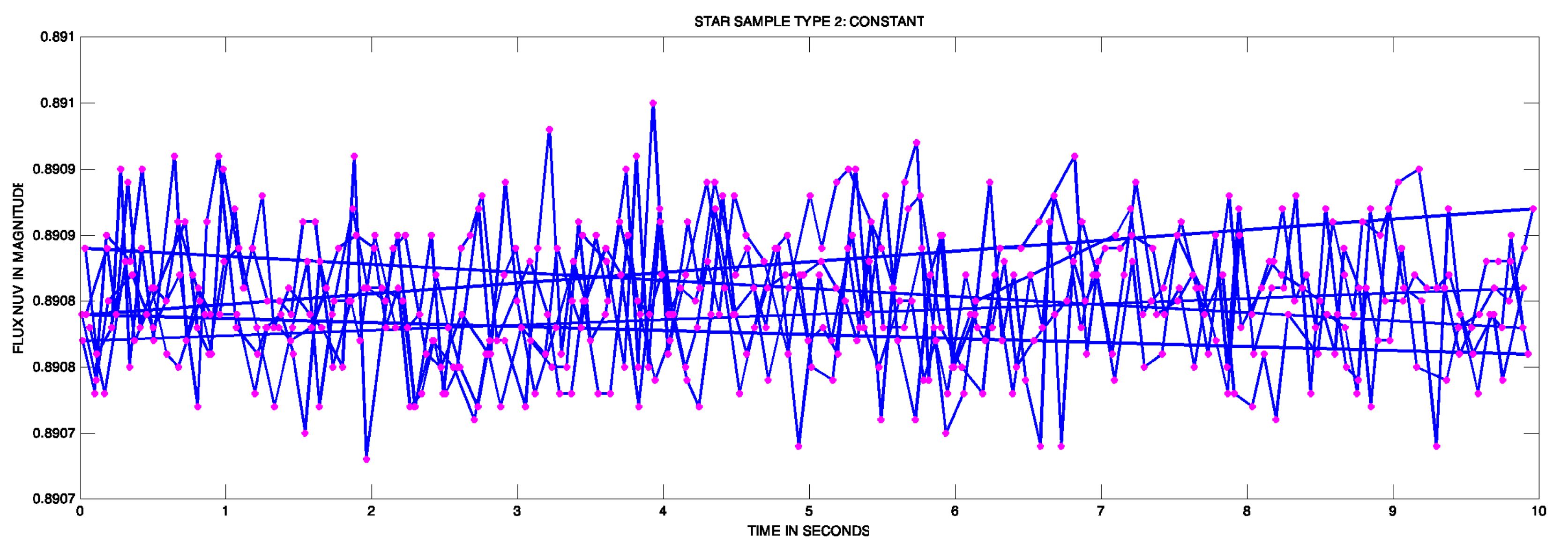
• Group 2 CONSTANT: Constant.
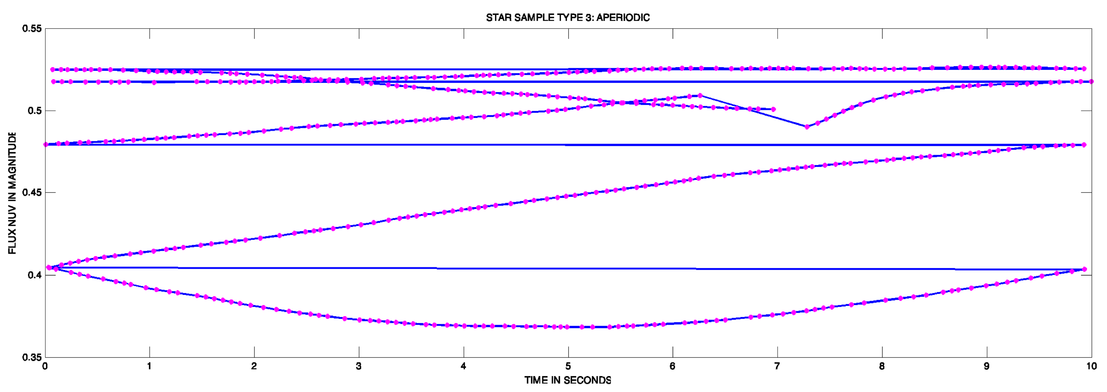
• Group 3 APERIODIC: Aperiodic and Long Period.
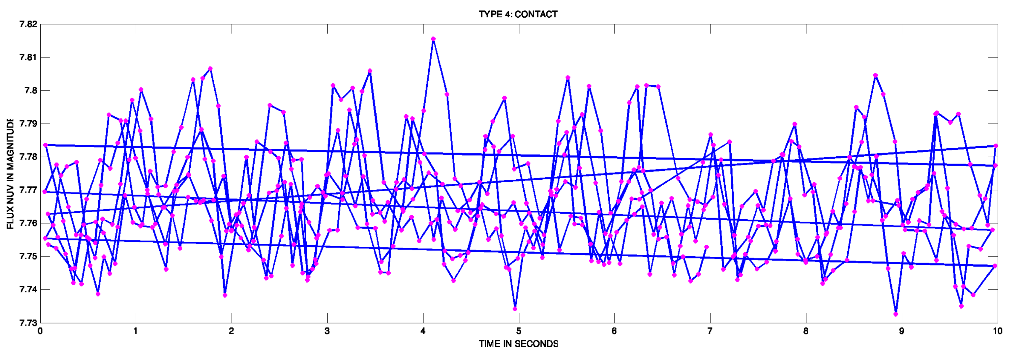
• Group 4 CONTACT-ROT (Rotational): Rotational and Binary Contact, including Chemically Peculiar.
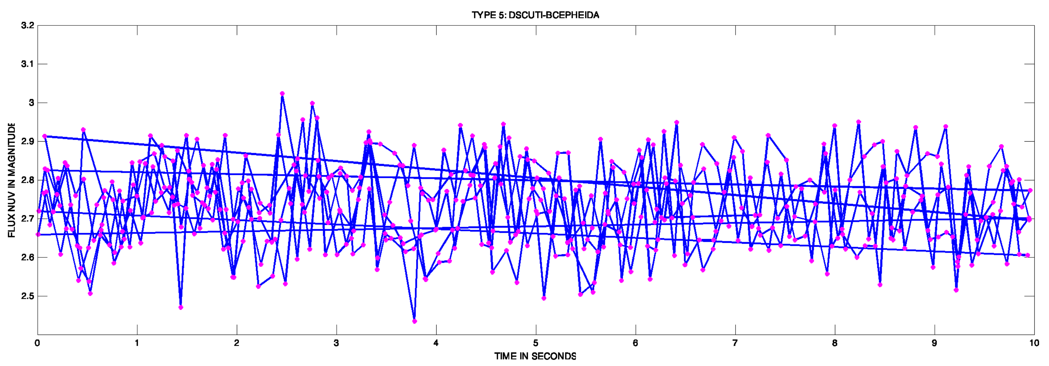
• Group 5 DSCT-BCEP: Delta Scuti (DSCT) and $\beta$ Cepheids (BCEP).
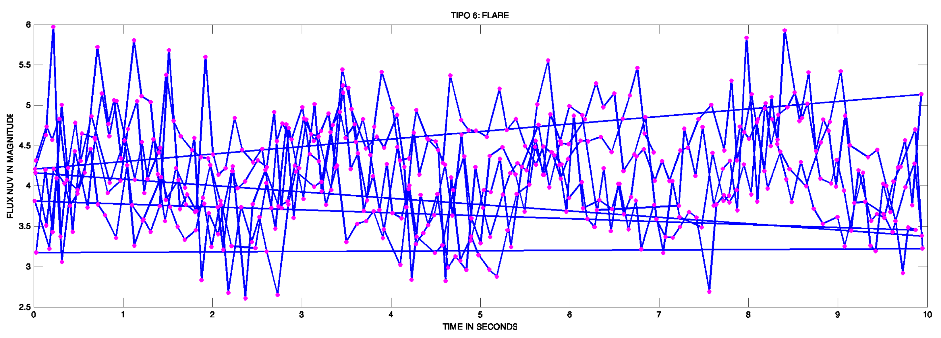
• Group 6 FLARE: Stars with Transient Outbursts or Flares.
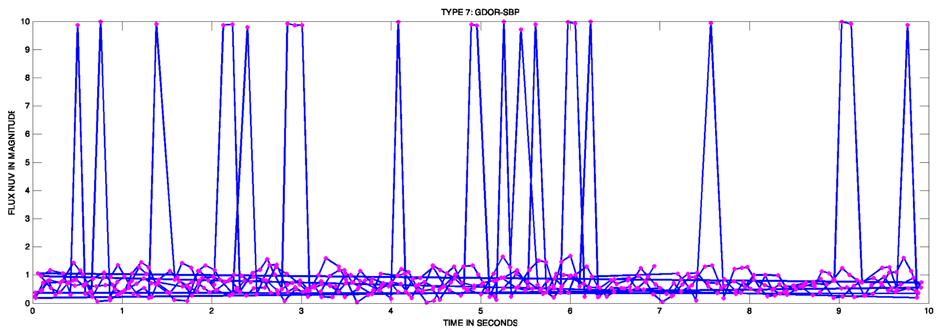
• Group 7 GDOR-SPB: Gamma Doradus (GDOR) and Slowly Pulsating B-type (SPB) stars.
• Group 8 RRLYR-CEPHEID: RRLyrae (RRLYR) stars and Cepheid Variables (CEPHEID).
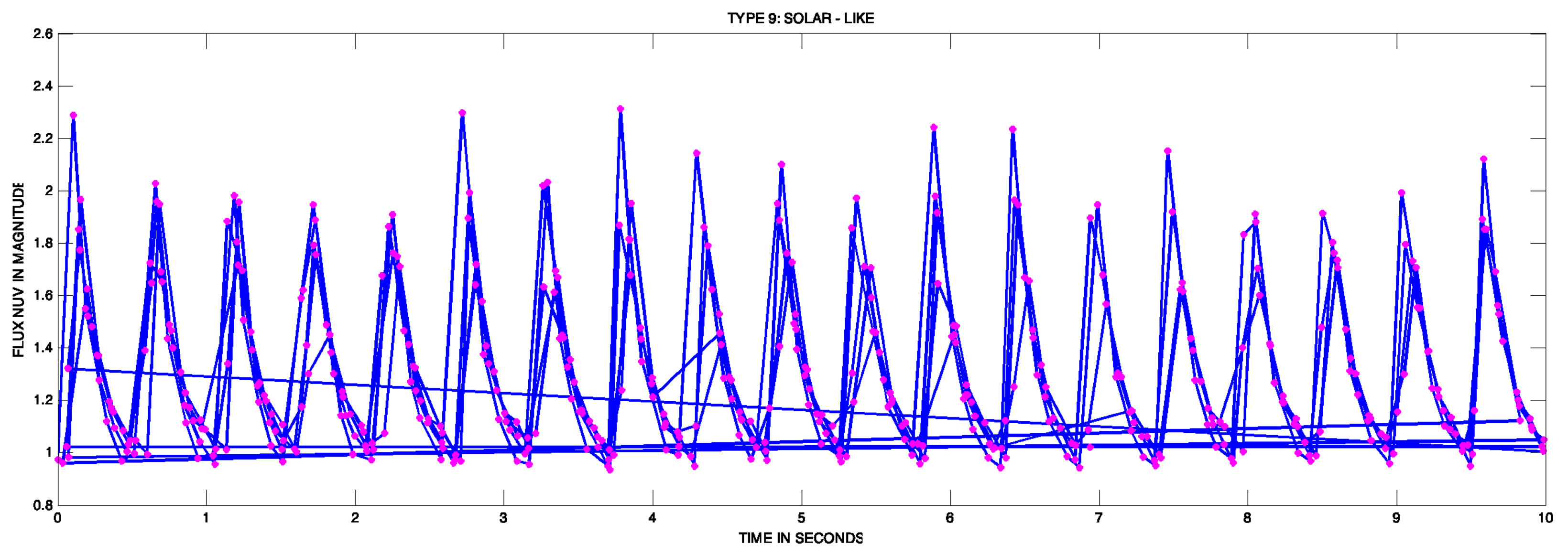
• Group 9 SOLAR-LIKE: Solar-like stars.

This classification is performed using three distinct neural network architectures:

1.

Applying a backpropagation neural network algorithm with pre-labeled samples under a multilayer perceptron architecture with supervised learning, consisting of 17 input nodes, five hidden nodes, and nine output nodes [10].

2.

Applying a backpropagation neural network algorithm with pre-labeled samples under a multilayer perceptron architecture with supervised learning, consisting of 17 input nodes, 10 hidden nodes, and nine output nodes [10].

3.

Applying a backpropagation neural network algorithm with pre-labeled samples under a multilayer perceptron architecture with supervised learning, consisting of 17 input nodes, 15 hidden nodes, and nine output nodes [10,11,12].

The final result will be a catalog of new datasets labeled with their respective categories and quantification data with a certainty percentage above 30%. The Figure 1 shows the Methodology for Classifying Kepler Light Curves Using Artificial Intelligence.

3. Experiments

We will initiate our process with the collection of Kepler data and the classification of stellar variability categories. Following that, we will outline the experimental setup.

3.1. Kepler Data Collection

The collection contains 760 samples of stars that covers 9 types of stars, this collection includes observation time, the NUV flux, and the error (signal to noise error) of the flux. The categories considered in 15 data sets defined as follows in

Table 2. Star data sets show different errors and resolutions.

Data Set	No. Data	No. Points	Error Value	File Name
1	9880	13	00	mgck_ab_n013_e00.xlsx
2	9880	13	05	mgck_ab_n013_e05.xlsx
3	9880	13	10	mgck_ab_n013_e00.xlsx
4	15,200	20	00	mgck_ab_n020_e00.xlsx
5	15,200	20	05	mgck_ab_n020_e05.xlsx
6	15,200	20	10	mgck_ab_n020_e10.xlsx
7	38,000	50	00	mgck_ab_n050_e00.xlsx
8	38,000	50	05	mgck_ab_n050_e05.xlsx
9	38,000	50	10	mgck_ab_n050_e10.xlsx
10	114,000	150	00	mgck_ab_n150_e00.xlsx
11	114,000	150	05	mgck_ab_n150_e05.xlsx
12	114,000	150	10	mgck_ab_n150_e10.xlsx
13	342,000	450	00	mgck_ab_n450_e00.xlsx
14	342,000	450	05	mgck_ab_n450_e05.xlsx
15	342,000	450	10	mgck_ab_n450_e10.xlsx

.

Each type of variability is trained with 100 examples, except the APERIODIC class, which includes only 28 examples, and the RRLYR—CEPHEID class, which has 32 training examples. The table Table 2 provides detailed information on this topic.

As illustrated in Table 2, the data is divided into 15 sets, each containing multiple data points and a corresponding error value.

The classification approach employs an ensemble method that runs multiple algorithms independently to enhance classification accuracy. Specifically, we use the Bagging-Performance Approach Neural Network (BAPANN), a modified bagging technique. This method executes three neural network algorithms independently, each with a different number of hidden nodes (5, 10, and 15). The neural network with the highest classification percentage and a performance value closest to zero is selected as the best performer. This performance is demonstrated when the histogram in Figure 2 calculates errors as the difference between targets and outputs based on the learning achieved as the number of training samples increases (which are shown in blue).

The Bagging-Performance Approach Neural Network (BAPANN) is illustrated in Figure 2.

The core of BAPANN uses a Multilayer Perceptron architecture with backpropagation learning, a well-established model known for its high classification performance. This model often achieves accuracies above 80%, ensuring that our classifications are optimized for performance and accuracy.

3.2. Stellar Variability Categories

Each type of stellar variability is defined and must be recognized for the artificial intelligence code. This research aims to classify nine groups of stellar variability using optical flows that simulate ultraviolet photometry. A sample of each of the nine variables to be recognized is graphed from Figure 3, Figure 4, Figure 5, Figure 6, Figure 7, Figure 8, Figure 9, Figure 10 and Figure 11. It is essential to highlight that the dataset was carefully selected. However, some crossover can be seen in the data due to instrument noise and interruptions in readings between points during the sampling process. Nonetheless, it is confirmed that the neural network models are robust to disturbances, uncertainty, and noise within the dataset. Their performance is not adversely affected during the training or learning stages.

The definitions for these groups are provided below:

• Group 1 ECLIPSE—Binary Eclipsants and Transit Events: Eclipsing/transiting (transit/eclipse) systems are a class of objects that exhibit extrinsic variability in the form of periodic changes in transits/eclipses [5]. An example of the light curve is illustrated in Figure 3.
• Group 2 CONSTANT—Constant: Constant stars (constant) are a class of objects that do not show any statistically significant variability on the timescale of 27.5 days [5]. An example of the light curve can be seen in the Figure 4.
• Group 3 APERIODIC—Aperiodic and Long Period: aperiodic variable stars refer to stars that do not exhibit any regular or repeating pattern in their brightness changes over time as Mira and Semiregular (Concepts according to the American Association of Variable Star Observers (AAVSO) An example of the light curve can be seen in the Figure 5.
• Group 4 CONTACT-ROT—Rotational and Binary Contact: Another geometric variability is caused by the star’s rotation. Rotating or rotational variables are stars that dim by a few percent as they rotate due to starspots [13] where 450 dots in 10 months were taked, and the value in flux of near ultraviolet band is meassured in axes x and y respectively.

On the other hand, Chemically Peculiar stars have a period of variability equal to the star’s rotation period. Chemically peculiar (CP) stars are a class of stars with distinctly unusual abundances of metals, at least in their surface layers, according to the research projects outlined in the first search result [13], a sample of this light curve is illustrated in Figure 6.

• Group 5 DSCT-BCEP—Delta ($\delta$) Scuti and ($\beta$) Cepheids: The stars $\beta$ Cepheids (Delta $\left(\delta \right)$ Scuti/$\left(\beta \right)$ Cepheids) are two pulsating variables in modes of radial and non-radial pressure of low order and gravity that are excited mainly through the mechanism that acts in the zone of partial ionization of helium (Delta $\left(\delta \right)$ Scuti stars) and the iron group. Beta $\left(\beta \right)$ Cep stars have masses between 8 and 25 Me, and their pulsation periods range from 2 to 8 h. The less massive Delta $\left(\delta \right)$ Sct stars cover the 1.5 to 2.5 Me mass range and have periods of about 15 min to about 8 h. Therefore, there is a significant overlap between the two in terms of pulsation periods [5]. A sample of this type of star, in its curve light, is the Figure 7.
• Group 6 FLARE—Transient or Flare Stars: The flares are believed to occur due to a magnetic reconnection event that creates a beam of charged particles that impacts the stellar photosphere, generating rapid heating and emission at almost all wavelengths. Although the initial heating produces a very hot gas, the flare is more pronounced in short wavelengths: ultraviolet and X-rays [14]. One sample of how looks a curve light of this type is Figure 8.
• Group 7 GDOR-SPB—Gamma ($\gamma$) Doradus and Slow Pulse: Gamma Doradus stars are a type of variable star that exhibits variations in luminosity due to non-radial pulsations in their surface layers [15]. An example of the curve light is shown in Figure 9.
• Group 8 RRLYR-CEPHEID—RRLyras and Cepheid Stars: Classical pulsators (class RRLyr—Ceph) are low to intermediate mass evolved stars whose intrinsic pulsation variability is driven by the opacity mechanism acting in the zone partial ionization of helium [5]. An example of the light curve can be observed in Figure 10.
• Group 9 SOLAR LIKE—Solar Like Stars: Solar-like pulsators (solar class) are intrinsically variable stars showing oscillations driven by turbulent convective motions near their surfaces. Any star with an outer convective zone is expected to show such stochastically excited oscillations [5]. An example of a light curve can be observed in Figure 11.

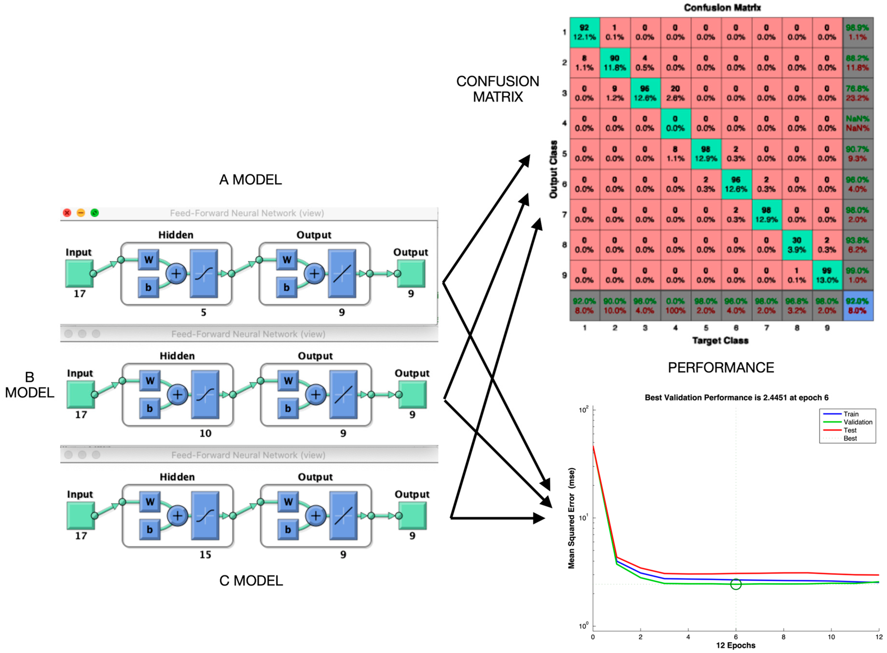
4. Results

The BAgging-Performance Approach Neural Network (BAPANN) training process involves an initial training session to test the classification level that BAPANN can achieve. It was initially tested with 760 stars, each with 13, 20, 50, 150, and 450 light points to be classified. Light points with 00, 05, and 10 errors were considered.

The set initially comprised 27 statistics. However, some statistics hindered the training of the BPANN. After a study of discriminant and non-discriminant features, the input was reduced to 17 parametric statistics.

The selection of the number of nodes is based on a recommendation used by [10], where it is suggested that the number of hidden nodes should be around 50% of the number of input nodes. For our case, 17 input nodes imply approximately 8.5 hidden nodes, rounded to 10. Therefore, we tested this recommendation (10 hidden nodes) and varied it with an upper bound of 15 and a lower bound of 5 hidden nodes. Its variability was chosen to prevent overtraining and ensure stable learning even if some architectures fail to learn the data examples correctly. Our methodology trained three architectures for 46 training tests:

(a)

BAPANN configuration 1: Containing 17 input nodes, five hidden nodes, and nine output nodes (17-5-9 configuration).

(b)

BAPANN configuration 2: Containing 17 input nodes, 10 hidden nodes, and nine output nodes (17-10-9 configuration).

(c)

BAPANN configuration 3: Containing 17 input nodes, 15 hidden nodes, and nine output nodes (17-15-9 configuration).

The results were obtained through an initial setup to select discriminant features, followed by a second configuration in Parametric Statistics, a Test of the Training Process, and an Analysis of Confusion Matrices.

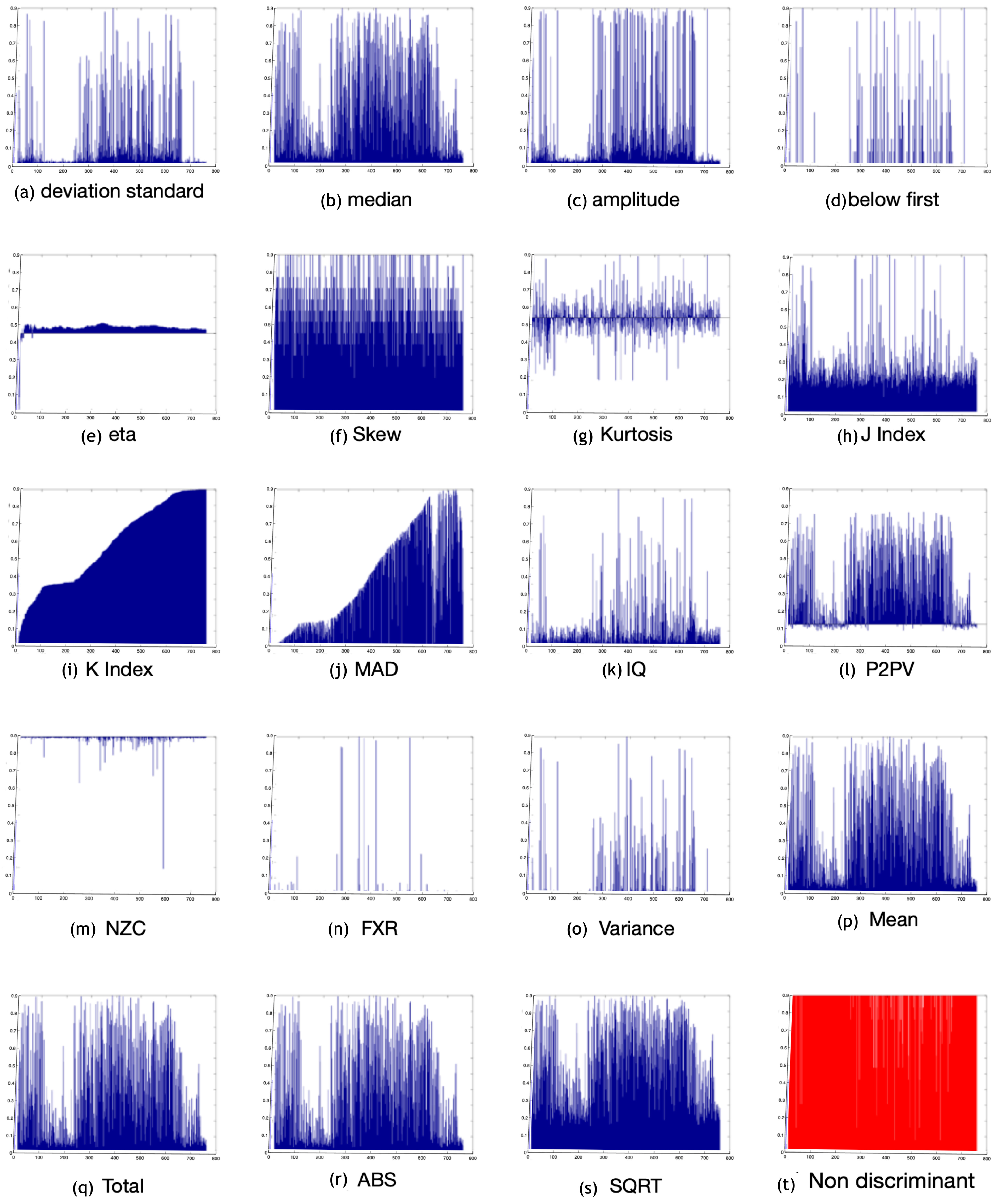
4.1. Initial Setup to Choose Discriminant Features

The advantage of the BAPANN approach is that features can be corrected by carefully analyzing the 27 statistics and separating discriminant from non-discriminant ones. An analysis was conducted, and each statistic was graphed to visually identify those relevant to learning and eliminate those that hinder it. Non-discriminant statistics are those that appear red in Figure 12, and this is because no variations are observed in their graphs, that is, their feature vector is completely continuous and unchanged.

The non-discriminant ($\mathcal{ND}$) statistics were identified and removed, which do not contribute to the neural network’s classification process. This left 17 discriminant ($\mathcal{D}$) statistics that influence the classification process.

$$\begin{array}{c}\hfill \left(\mathcal{ND}\right)=\{\mathcal{BYF},\mathcal{SSD},\mathcal{MXS},\mathcal{MDS},\mathcal{ASLP},\mathcal{CON},\mathcal{ROMS},\mathcal{PPV},\mathcal{S}\}\end{array}$$

(1)

where $\left(\mathcal{ND}\right)$ means non-discriminant features, such as $\mathcal{BYF}$ (beyond the first), $\mathcal{SSD}$ (Sum of Square Standard Deviation), $\mathcal{MXS}$ (Max Slope), $\mathcal{MDS}$ (Median Slope), $\mathcal{ASLP}$ (Absolute Slope), $\mathcal{CON}$ (Consecutive points), $\mathcal{ROMS}$ (absolute of the total of the flux and the product of the inverse of the number of points in the observation), $\mathcal{PPV}$ (ratio of differences and sum between maximum and minimum of flux and errors), and $\mathcal{S}$ (Sign).

$$\begin{array}{c}\hfill \left(\mathcal{D}\right)=\{\sigma ,\tilde{x},\omega ,\mathcal{BLF},\eta ,\mathrm{Kurtosis},\mathcal{JINDX},\mathcal{KINDX},\\ \hfill \mathcal{MAD},\mathcal{IQ},\mathcal{NZC},\mathcal{FXR},{\sigma }^2,\mathcal{AVG},\mathcal{TOT},\mathcal{ABS},\mathcal{SQRT}\}\end{array}$$

(2)

where $\left(\mathcal{D}\right)$ means discriminant features, such as $\sigma$ (standard deviation), $\tilde{x}$ (median flux), $\omega$ (amplitude), $\mathcal{BLF}$ (below the first), $\eta$ (third power of the difference between two successive flux values), Kurtosis (rth moment about the mean), $\mathcal{JINDX}$ (J index), $\mathcal{KINDX}$ (K index), $\mathcal{MAD}$ (median of the differences between the flux and the median of the flux), $\mathcal{IQ}$ (interquartile range), $\mathcal{NZC}$ (non-zero crossing), $\mathcal{FXR}$ (flux ratio), $\mathcal{AVG}$ (average), $\mathcal{TOT}$ (total flux), $\mathcal{ABS}$ (absolute), and $\mathcal{SQRT}$ (square root).

An example of the discriminant statistics $\left(\mathcal{D}\right)$ selected, along with an example of non-discriminant statistics, can be seen in Figure 12.

4.2. Second Configuration in Parametric Statistics

Once it was established which statistics were effective for classification, the type of architecture for more robust training was determined. Seventeen statistics were identified as adequate for training, leading to the three BAPANN architectures detailed above.

Some training sessions revealed that the $\mathcal{PPV}$ characteristic yielded values too small to be considered relevant for learning when the data sets contained 50, 150, or 450 light points per star curve. In such cases, $\mathcal{AVG}$, $\mathcal{TOT}$, and $\mathcal{ABS}$ were eliminated from the input training set, leaving only 17 statistics for tests 20 and 21, achieving the highest classification accuracy of 97.8% for nine stellar variability types for 760 stars (see

Table 3. Star datasets are provided at different error levels and resolutions for training purposes.

Group No.	Variability Type	No. Samples
1	ECLIPSE	100
2	CONSTANT	100
3	APERIODIC	28
4	CONTACT	100
5	DSCT-BCEP	100
6	FLARE	100
7	GDOR-SPB	100
8	RRLYR-CEPHEID	32
9	SOLAR-LIKE	100
	TOTAL	760

).

4.3. Test of Training Process

The training was performed for each data set with the 3 BAPANN architectures detailed above. Each test displayed the following elements: 1. The trained architecture: BAPANN Architecture 1, 2, or 3, 17 input nodes, nine output nodes, and varying hidden nodes. 2. The number of epochs required for each architecture to learn the data set. 3. The classification percentage obtained for each case. 4. The performance of the neural network.

Forty-five detailed tests are described in

Table 4. Correct classification by class and by instances of the five matrices chosen as those that yielded a classification percentage near 99%. (* In this test, only 17 statistics were required, for which (1) Average, (2) Total, and (3) Absolute are removed for the input data). Where dots indicate the resolution of the light curve.

Run	Epochs	Dots and SNR	Hidden Nodes	Percentage
6	18	13$\times {10}^{-5}$	15	92.0%
12	45	20$\times {10}^{-0}$	15	96.6%
20	68	50$\times {10}^{-0}$	10	97.8% *
32	34	150$\times {10}^{-5}$	10	95.1%
45	70	450$\times {10}^{-10}$	15	98.9%

. Additionally, the update operations of the hidden nodes are shown in expression (3):

$$z_{iactiv}={\displaystyle \frac{1}{1+exp(-z_i)}}$$

(3)

where $z_{iactiv}$ means the output of hidden nodes activation function, $z_i$ means the output of hidden node $z_i$.

4.4. Analysis of Confusion Matrices

The confusion matrices provide insights into the percentage of correct or incorrect classifications, false positives, and false negatives and help identify complex categories for the model to classify. This information may indicate the need to reconsider some categories or reinforce the model architecture. Five examples of confusion matrices, yielding percentages of 92.6%, 96.8%, 97.8%, 96.1%, and 97.4% for the 9 cases of stellar variability, are shown in Figure 13 and Figure 14a.

In particular, it is observed that the class that obtains a percentage of 0% classification is GROUP 3 APERIODIC stars, as is shown in some of the confusion matrix in Figure 14a.

Below is Table 4 with the best percentages selected for different cases, and where DOTS means the number of points that describe the light curve, and this is a function of that data set and its corresponding error where the best percentage was achieved among the 15 light curve data sets handled. This is due to the error of the instrument providing the data based on noise or static of the signal or telescope. Although this does not affect the operation of the classifier through the assembly of neural networks, it does affect their aesthetics visually in the graphs. However, this does not prevent effective classification. It is demonstrated that despite these details in the light curve samples, the ensemble omitted or suppressed the uncertainty, ambiguity, or noise in the data due to static or instrument measurements. The effect is not of significant importance in the classification process performed by the neural networks.

5. Conclusions

It is essential to mention that for datasets with fewer points on the light curve, the classification percentage decreases more significantly than in cases where the number of points on the light curve is more significant. Another determining factor is the noise error in the signal accompanying each dataset. This indicates that the smaller the dataset and the greater the noise, the more complex the classification. Another observation regarding classification indicates that having more nodes in the hidden layer can improve learning, which also leads to an improvement in the classification percentage. On the other hand, input feature selection must be carefully selected to visually distinguish discriminatory ones, which helps improve learning or even accelerate it and avoid overtraining. The architectures with higher percentages have 10 to 15 nodes in the hidden layer, while the architecture with five nodes does not achieve the highest percentages. Our findings suggest that achieving percentages of up to 91% with only 13 light curve points demonstrates that the BAPANN model, in architectures 2 and 3 (with 10 and 15 hidden nodes, respectively), are reliable models for categorizing stellar variability using only 17 features for the input layer (parametric statistics). It has been observed that with 50 light curve points, it is sufficient to classify eight types of stellar variability, which surpasses all the reviewed state-of-the-art. A maximum correct classification rate of 98.9% is achieved, and in the best case, 97.8%. Both values are above the state-of-the-art maximum of 94.9%. The most effective architecture in our BAPANN ensemble is a Multilayer Perceptron architecture trained with a backpropagation algorithm with 10 hidden nodes. This is improved even with just 17 carefully selected statistics, where achieving percentages above 90% is possible.

References

1. Debosscher, J.; Sarro, L.M.; Aerts, C.; Cuypers, J.; Vandenbussche, B.; Garrido, R.; Solano, E. Automated supervised classification of variable stars-I. methodology. Astron. Astrophys. 2007, 475, 1159–1183. [Google Scholar] [CrossRef]
2. Olmedo, M.; Lloyd, J.; Mamajek, E.E.; Chávez, M.; Bertone, E.; Martin, D.C.; Neill, J.D. Deep GALEX UV Survey of the Kepler Field. I. Point Source Catalog. Astrophys. J. 2015, 813, 100. [Google Scholar] [CrossRef]
3. Bass, G.; Borne, K. Supervised ensemble classification of Kepler variable stars. Mon. Not. R. Astron. Soc. 2016, 459, 3721–3737. [Google Scholar] [CrossRef]
4. Olmedo Aguilar, N.D. Fuentes Variables Ultravioleta en el campo de Kepler. PhD Thesis, INAOE, San Andrés Cholula, Mexico, 2017. [Google Scholar]
5. Audenaert, J.; Kuszlewicz, J.S.; Handberg, R.; Tkachenko, A.; Armstrong, D.J.; Hon, M.; Kgoadi, R.; Lund, M.N.; Bell, K.J.; Bugnet, L.; et al. TESS data for asteroseismology (T’DA) stellar variability classification pipeline: Setup and application to the Kepler Q9 data. Astron. J. 2021, 162, 209. [Google Scholar] [CrossRef]
6. Barbara, N.H.; Bedding, T.R.; Fulcher, B.D.; Murphy, S.J.; Reeth, T.V. Classifying Kepler light curves for 12,000 A and F stars using supervised feature-based machine learning. Mon. Not. R. Astron. Soc. 2022, 514, 2793–2804. [Google Scholar] [CrossRef]
7. Miles, B.E.; Shkolnik, E.L. HAZMAT. II. Ultraviolet variability of low-mass stars in the GALEX Archive. Astron. J. 2017, 154, 67. [Google Scholar] [CrossRef]
8. Kim, S.T.; Cai, W.; Jin, F.F.; Yu, J.Y. ENSO stability in coupled climate models and its association with mean state. Clim. Dyn. 2014, 42, 3313–3321. [Google Scholar] [CrossRef]
9. Wittenmyer, R.A.; Butler, R.P.; Tinney, C.G.; Horner, J.; Carter, B.D.; Wright, D.J.; Jones, H.R.; Bailey, J.; O’Toole, S.J. The Anglo-Australian planet search XXIV: The frequency of Jupiter analogs. Astrophys. J. 2016, 819, 28. [Google Scholar] [CrossRef]
10. Fausett, L.V. Fundamentals of Neural Networks: Architectures, Algorithms, and Applications; Prentice-Hall: Hoboken, NJ, USA, 1994. [Google Scholar]
11. Rokach, L. Pattern classification using ensemble methods. Ser. Mach. Percept. Artif. Intell. 2010, 75, 225. [Google Scholar]
12. Sewell, M. Ensemble learning. Res Note 2008, 11, 1–34. [Google Scholar]
13. Preston, G.W. The chemically peculiar stars of the upper main sequence. Annu. Rev. Astron. Astrophys. 1974, 12, 257–277. [Google Scholar] [CrossRef]
14. Segura, A.; Walkowicz, L.M.; Meadows, V.; Kasting, J.; Hawley, S. The effect of a strong stellar flare on the atmospheric chemistry of an Earth-like planet orbiting an M dwarf. Astrobiology 2010, 10, 751–771. [Google Scholar] [CrossRef] [PubMed]
15. Antoci, V.; Cunha, M.S.; Bowman, D.M.; Murphy, S.J.; Kurtz, D.W.; Bedding, T.R.; Borre, C.C.; Christophe, S.; Daszyńska-Daszkiewicz, J.; Fox-Machado, L. The first view of δ Scuti and γ Doradus stars with the TESS mission. Mon. Not. R. Astron. Soc. 2019, 490, 4040–4059. [Google Scholar] [CrossRef]
Figure 1. Methodology for Classifying Kepler Light Curves Using Artificial Intelligence.
Ai 06 00102 g001
Figure 2. The Bagging-Performance Approach Neural Network (BAPANN) is an ensemble system built from three neural networks configured with different numbers of hidden nodes. The optimal architecture is determined by evaluating each network’s confusion matrices and performance metrics based on the training set.
Ai 06 00102 g002
Figure 3. The light curve of a Group 1 star, specifically an eclipse event, consists of 450 data points collected over 27.5 days. The flux value is measured in terms of the ultraviolet light magnitude, which is represented on the y-axis. The x-axis denotes the exposure time in seconds.
Ai 06 00102 g003
Figure 4. The light curve of a Group 2 star, which exhibits a constant flux, consists of 450 data points collected over 27.5 days. The flux value is measured in terms of the ultraviolet light magnitude, represented on the y-axis, while the x-axis indicates the exposure time in seconds.
Ai 06 00102 g004
Figure 5. The light curve of a Group 3 star, characterized by aperiodic behavior, consists of 450 data points collected over 27.5 days. The flux value is measured in terms of the ultraviolet light magnitude, represented on the y-axis, while the x-axis denotes the exposure time in seconds.
Ai 06 00102 g005
Figure 6. The light curve of a Group 4 star, specifically exhibiting Contacto-Rot behavior, consists of 450 data points collected over 27.5 days. The flux value is measured in terms of the ultraviolet light magnitude, represented on the y-axis, while the x-axis indicates the exposure time in seconds.
Ai 06 00102 g006
Figure 7. The light curve of a Group 5 star, exhibiting Dsct-BCepheid characteristics, consists of 450 data points collected over 27.5 days. The flux value is measured in terms of the ultraviolet light magnitude, represented on the y-axis, while the x-axis indicates the exposure time in seconds.
Ai 06 00102 g007
Figure 8. The light curve of a Group 6 star, identified as a Flare star, comprises 450 data points collected over 27.5 days. The flux value, measured in ultraviolet light magnitude, is represented on the y-axis, while the x-axis indicates the exposure time in seconds.
Ai 06 00102 g008
Figure 9. The light curve of a Group 7 star, classified as Gdor-SPB, consists of 450 data points collected over 27.5 days. The flux value, measured in terms of ultraviolet light magnitude, is represented on the y-axis, while the x-axis signifies the exposure time in seconds.
Ai 06 00102 g009
Figure 10. The light curve of a Group 8 star, identified as RRLyrae-Cepheid, comprises 450 data points collected over 27.5 days. The flux value, measured in ultraviolet light magnitude, is represented on the y-axis, while the x-axis indicates the exposure time in seconds.
Ai 06 00102 g010
Figure 11. The light curve of a Group 9 star, classified as Solar-like, consists of 450 data points collected over 27.5 days. The flux value, measured in terms of ultraviolet light magnitude, is represented on the y-axis, while the x-axis indicates the exposure time in seconds.
Ai 06 00102 g011
Figure 12. Discriminant statistics and an example of non-discriminant statistics. The blue graphs shows skews (are discriminants), but red graphs shows filled axes (not discriminants). The x axes represents the 760 star samples. The y axes represents the value of the statistic mentioned between 0 and 1 real valued. A discriminant statistic displays variations in its graph (blue), whereas a non-discriminant statistic shows a continuous graph (red).
Ai 06 00102 g012
Figure 13. 4 Confusion matrix (CM) of percentages of 92.0 %, 96.6 % 97.8 % and 95.1% recognized instances.
Ai 06 00102 g013
Figure 14. (a) Confusion matrix resulting from test 9 with 98.9% (blue square) recognized instances. (b) Convergence of learning performance reached epoch 17 with a value of 0.62753. (c) Example of a histogram of learning errors in 20 test containers, achieving a minimum error of 0.2167, which reflects that the difference between the labels and what the model learns is very close to 0. (d) Stellar variability classification of 760 stars, represented in 3 dimensions, with x = mean ( x ˜ ), y = amplitude (w) and z = stellar variability class.
Ai 06 00102 g014