The Artificial Intelligence Quotient (AIQ): Measuring Machine Intelligence Based on Multi-Domain Complexity and Similarity

Abstract

The development of AI systems and benchmarks has been rapidly increasing, yet there has been a disproportionately small amount of examination into the domains used to evaluate these systems. Most benchmarks introduce bias by focusing on a particular type of domain or combine different domains without consideration of their relative complexity or similarity. We propose the Artificial Intelligence Quotient (AIQ) framework as a means for measuring the similarity and complexity of domains in order to remove these biases and assess the scope of intelligent capabilities evaluated by a benchmark composed of multiple domains. These measures are evaluated with several intuitive experiments using simple domains with known complexities and similarities. We construct test suites using the AIQ framework and evaluate them using known AI systems to validate that AIQ-based benchmarks capture an agent’s intelligence.

1. Introduction

Deciding whether an AI system is intelligent has been a challenge since the creation of computing machines. The initial standard method for determining intelligence, the Turing Test [1], has fallen out of favor due to the rapid development of AI systems and the test’s subjectivity. With so many robust systems currently in use today, researchers need a more objective method for determining the intelligence and performance of an AI system. Several recent benchmarks have emerged, motivated by the need to evaluate and compare Large Language Models (LLMs). However, they are specialized to the question-answering paradigm, and little analysis has been done on the similarity and relative difficulty of the individual tests in the benchmarks. There is not yet a standard framework or testing system that has been widely adopted by researchers in the field to quantify a system’s intelligence.

While the progress of AI systems and their capabilities has rapidly increased, these systems often specialize on a single task and are often not generalizable. This lack of generalizability can be so severe that even a small shift in a domain can cause significant performance decreases. This issue is commonly referred to as “brittleness”. One explanation for this behavior is the lack of adaptation capabilities in AI systems. This is the result of making a closed world assumption [2]. One example of this behavior can be observed in the Dota playing AI system “OpenAI Five” [3]. While OpenAI Five achieved superhuman performance when played in a rigid environment, it was unable to adapt to subtle changes in gameplay when exposed to the community. This resulted in very simple exploits to defeat the system to which human players can easily adapt. Brittleness is not limited to reinforcement learning systems but is also found in classification-based AI systems [4]. Brittleness is especially important in safety critical systems where environmental shifts can cause potentially fatal results [5].

We propose a framework for measuring intelligence that can be used to increase our understanding of AI systems and create more generalizable benchmarks. This is achieved with two domain measures, dissimilarity and complexity. When these measures are combined, we can create an objective space of domains within which to define intelligence. We can then evaluate a given AI system’s ability in this space and generate its Artificial Intelligence Quotient (AIQ). The AIQ provides a more granular understanding of how an AI system is performing and a better measurement of the AI system’s generalizability.

These domain measurements allow for the creation of an intelligence space. Once a test is located in the space, its performance metric is used to scale that position. This scaling represents the agent’s capacitance, or its ability to achieve a specific understanding of the domain. An agent that achieves a higher understanding of the domain will be given a higher AIQ score than one that achieves a lower understanding. Agent capacitance also scales with domain complexity. An agent that achieves a comparable understanding of a more complex domain will be given a higher AIQ score than an agent on a less complex domain.

While our aim in this paper is to introduce the AIQ framework rather than a full-scale benchmark, we note that applying AIQ to modern multimodal and large-scale tasks remains future work. We focus here on simpler domains with well-understood structure to clearly illustrate the behavior of the dissimilarity, complexity, and intelligence measures. Extending AIQ to richer environments and high-capacity AI systems is a natural next step and will further test the framework’s scalability and generality.

1.1. Existing Benchmarks

Several AI benchmarks already exist that focus on natural language processing, adaptation, and multiple domains. Natural Language Processing (NLP) benchmarks aim to test an agent’s ability to process and comprehend natural languages. A popular example is the General Language Understanding Evaluation (GLUE) benchmark [6]. GLUE is a collection of a diverse set of already existing language tasks. The objective of the benchmark is to test an agent’s capabilities while multi-tasking on many differing language style tasks. Other benchmarks have been constructed following GLUE such as SuperGLUE [7], AdvGLUE [8], and BREAK [9].

Another type of benchmark utilizes domains that present a known environment and introduce a modification to the environment to examine the agent’s adaptive capabilities. One example is Science Birds [10], based on the popular video game Angry Birds. Science Birds introduces several novel domain shifts that change the domain slightly to introduce a new mechanic or concept into the game. A number of newly created domains exist with a similar concept to evaluate agents in open-world environments, such as Polycraft [11], Monopoly [12], NovGrid [13], and CartPole3D [14].

A second type of evolving domain introduces novel domain shifts, but each shift is relevant to the next, e.g., introducing intermediate goals that need to be achieved before the end goal can be reached. One example is the Obstacle Tower domain [15]. The agent must learn in depth planning to solve the base domain and use adaptation to explore how novel introduced objects affect the environment. Other examples of such domains include Urban Combat Testbed [16] and Procgen [17]. These single and multiple shift domains are useful for determining adaptation capabilities in AI systems, but they still lack the ability to evaluate cross-domain generalization.

Multi-domain benchmarks could be utilized to evaluate cross-domain generalization. Some of these benchmarks include GLUE [6], SuperGLUE [7], GVGAI [18], and ALE [19]. One concern with these benchmarks is that they lack diversity by using only one type of problem, such as a focus on video game playing. This lack of diversity makes it more challenging to effectively evaluate AI systems with greater generalizability. Second, these benchmarks do not support the notion of test weighting and often just evenly or subjectively weight the domains. This can lead to systemic targeting of key tests for a greater score rather than rewarding an AI system that can handle diverse tests. The lack of diversity and ability to effectively weight domains are key issues we address in the AIQ framework by measuring the diversity and complexity of tests within the benchmark.

Several recent benchmarks have emerged, motivated by the need to evaluate and compare Large Language Models (LLMs). BIG-bench [20] and HELM [21] consist of large numbers of diverse tasks presented in a question-response paradigm ranging from simple knowledge retrieval to complex reasoning. AGIEval [22] includes a large breadth of human-centric IQ tests (e.g., SAT, GRE, …) to determine how AI systems compare to each other and to humans. Their results show that average human performance over many differing tests tends to be higher than the performance of AI systems, with the exception of math and SAT tests. Top human performance is still higher than any of the evaluated AI systems. This is one example of how a broad set of tests can be utilized to achieve a granular view on what aspects certain systems perform well on. These benchmarks are specialized to the question-answering paradigm and combine results using a simple average over task performance. They provide little analysis on the similarity and relative difficulty of the individual tasks.

Another recent benchmark is the Abstraction and Reasoning Corpus (ARC) [23]. ARC is similarly structured to Raven’s Progressive Matrices, a well-established intelligence test [24]. Each task in the domain consists of example images with a prior image and after image, where the after image is generated via some function. The goal of the task is to determine the transition function and apply it to the test images. The transition function ranges in complexity to allow both simple and complex policy systems to be evaluated. However, integrating existing tests can be difficult in terms of translating them into functions over images. While the ARC benchmark is promising for evaluating both humans and AI systems, it does not offer a measurement of generalization between tasks, i.e., their relative difficulty and uniqueness. ARC also does not provide a method to determine the extent of intelligent behavior evaluated by the benchmark. ARC is still useful for measuring intelligence as the benchmark is expansive both in terms of the complexity and the diversity of tasks.

Some valid criticisms of benchmarks have recently arisen [25], including that the domains are arbitrarily selected, limited in scope, and are not evaluating what is being claimed. Which has led to the current state of AI development where researchers often focus on achieving state-of-the-art performance and do not attempt to make generalizable systems.

1.2. Existing Frameworks

An intelligence measure should utilize a wide breadth of domains that vary in both type and difficulty. One solution would be to use every feasible test to measure the performance of the AI system. An implementation of this approach was constructed by Hernandez-Orallo and Dowe [26] using a finite set of environments, with appropriate characteristics, to create an intelligence measure. Carefully constructed toy domains were used in the evaluation process. While this methodology provides guidance on how to construct a measure from the theory, it relies on specifically created domains. A more effective approach would be to examine existing domains and integrate them into a measure without having to change their implementation.

One foundational work is the Universal Intelligence Measure [27]. In this work, Legg and Hutter construct a theoretical framework for evaluating the general intelligence of an AI system. This is achieved by running an agent over the set of all possible tests to achieve a score. This score is then weighed by the Kolmogorov complexity of the test. The final intelligence score of the agent is its weighted performance over all tests. However, this work is entirely theoretical and cannot be practically used as an effective measure.

Another implementation by Legg and Veness [28] utilized a random program generator to sample from the set of all domains. This method of random sampling is impractical to use at larger scales and suffers due to the low probability of randomly sampling a complex domain from the set of all domains. A more effective approach would be to perform a more systematic exploration of the set of all domains. Their work also provided an alternative to using a similarity metric. Instead of comparing pairs of tests, they consider a uniform distribution of tests over the set of all possible tests. Difficulty is estimated based on the AI system’s score on the tests, and similarity is estimated based on the difference between this score, and the score on the entire test set.

An approximation of this measure was constructed by Hernandez-Orallo and Dowe [29] by creating a program generator and converting each program into a reinforcement learning based environment. The Kolmogorov complexity of each environment was approximated and used to generate the final intelligence score. However, each individual test is mostly meaningless in terms of what is being evaluated, so we cannot resolve what aspects of intelligence on which the AI system is performing well or needs improvement. The approximation also requires an extremely large problem space to be explored before an accurate result can be given. In their work, a hundred thousand environments were utilized. Sampling from a more complex problem domain would require many more samples. They limit the tests to randomly-generated programs, but even representative subsets are too large to be practical for evaluation. And the programs do not necessarily relate to real-world problems.

More recent frameworks have emerged with more rigorous metrics and improved applicability [30], as well as better theories [31] and implementations [32]. While these methodologies have a firm theoretical basis, they are often too computationally intensive or difficult to integrate with existing systems and tests. They also require careful curation to ensure a diverse and challenging set of tests for the targeted AI system. A preferable approach is to map existing tests into a shared theoretical framework. This allows evaluations to scale in size and scope while retaining a rigorous foundation and reducing debate about which tests to include.

Although our initial test suite is limited in both size and scope, it serves as a proof of concept for applying the AIQ to existing domains. Since AIQ is designed to be generalizable and extendable, adding in additional domains will further increase the accuracy of results and allow for the evaluation of increasingly powerful AI systems. Results gathered with this initial test suite include only a few dimensions of intelligence, and only a minor measurement along each dimension. However, the process supports evaluating benchmarks with a focus on domain side measurements.

2. Materials and Methods

2.1. Definition of a Test

Here we define the meaning of a test. We generalize the concept of a test to allow for the use of other theories that already exist. Colloquially, a test is defined as a set of questions and answers. When these are combined along with some scoring method, they create a score for the system taking the test. Others have provided definitions of tests [27,28,29], but they impose many restrictions that hinder the generalizability of a test. We start with the most general definition of a test.

Definition 1

(Test). A test $t(Q,S)$ consists of a set of questions Q and a scoring function S. A system A given questions Q produces a set of responses $R=A\left(Q\right)$. The performance $V=S(Q,R)$ is the system A’s score on test t.

We also make two assumptions: (1) a test must be defined within a finite set of memory, and (2) a test must always conclude. The empty test ∅ is a test with no questions or information. At the other extreme, we can also determine the existence of a test which asks every combination of questions, which we call the everything test, denoted as $\mathbb{T}$. Individual tests can be combined into larger tests, or test suites, defining a subset hierarchy between ∅ and $\mathbb{T}$. In this work, we also use the term domain as synonymous with test.

This definition and assumptions allow us to transform a test into a program, which can be represented as a finite Turing machine. This will be important later when we consider the complexity of a test and the similarity between two tests.

2.2. Dimensions of Intelligence

We define the intelligence space I as the space of all tests, from the empty test ∅ to the everything test $\mathbb{T}$. The dimensionality is defined as the number of mutually exclusive concepts of intelligence. While we do not know everything about the dimensionality of the intelligence space, most assume it is both finite and small. Previous research into Carroll’s model [33] has suggested there are between 8 and 10 broad categories of intelligence but may include upwards of 20 [34].

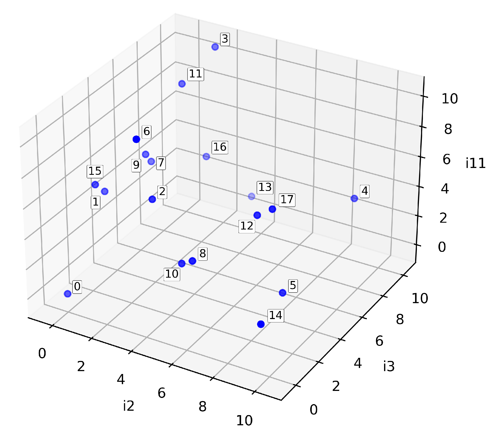
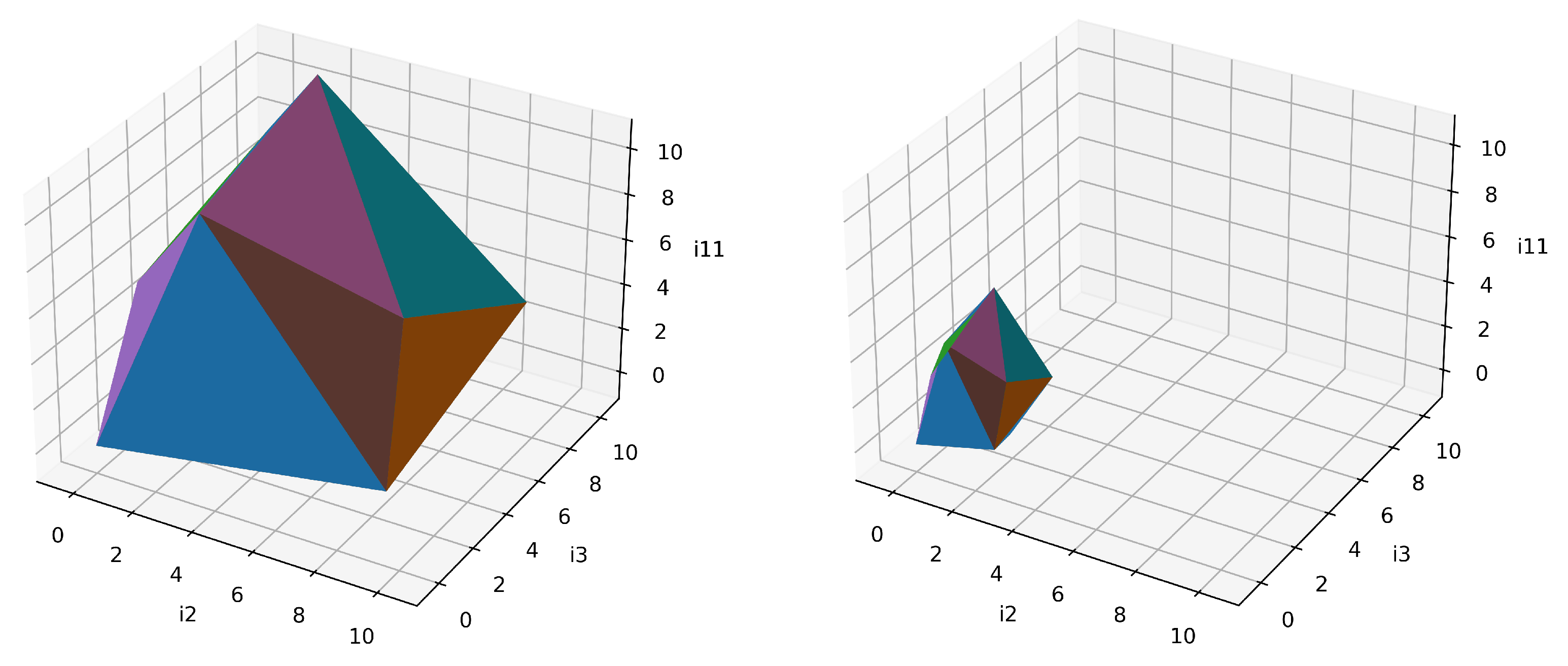
An example of an intelligence space is shown in Figure 1. The domain locations in the intelligence space are shown in Figure 1 (left). The test locations are then used to construct a shape in the intelligence space. A sample of what a shape in the space may look like is shown in Figure 1 (middle). The resulting volume enclosed by the shape is then the breadth and depth of intelligence being used to evaluate the AI system. An example agent is used to scale the shape shown in Figure 1 (middle), resulting in a much smaller shape containing a smaller volume, as shown in Figure 1 (right). A larger volume enclosed by the shape suggests an increase in breadth or depth is being evaluated. The shape is then scaled according to the AI system’s achieved performance on the domains in the test suite. A lower performance will decrease the depth of the shape, resulting in a smaller volume. The volume of the scaled shape is then the system’s AIQ score. More details on this example can be found in Section 3.4.4.

2.3. Agent Capacitance

Agent capacitance is similar to an agent’s capabilities, except that the capability of an agent is often described as a single performance value while capacitance is a multi-element value or vector. Capacitance is an agent’s ability to perform in the intelligence space and is defined as a scaled vector in the intelligence space.

$${\varphi }_t^{\pi }=\overrightarrow{V_{\pi }}{\mathit{I}}_t$$

(1)

where $\varphi$ is the capacitance of the agent $\pi$ for test suite t. $\overrightarrow{V_{\pi }}$ is the performance vector used to scale the subspace ${\mathit{I}}_t$ of intelligence space exercised by a test suite t.

AIQ [35] is a theoretical framework for measuring an agent’s capacitance on the intelligence space enclosed by some test suite. It combines a notion of complexity and dissimilarity to locate where tests are in the intelligence space.

2.4. Complexity

2.4.1. Definition

We define complexity based on the intelligence space as the amount of capacity a system needs to solve a given task. A task is more complex if it requires a larger capacity system to achieve the same performance as an easier task.

Definition 2

(Complexity). The complexity C of a domain μ is defined as the sum of the minimum capacitance ϕ required to achieve a performance value $V_{\mu }$ over the possible range of performance values of the domain.

Complexity in regards to the intelligence space is defined slightly differently, but it is still the same concept. The complexity of a domain in the intelligence space can be given as the magnitude of the vector in the intelligence space. This is more clearly defined in the following equation:

$$C\left(\mu \right)=\Vert \overrightarrow{I_{\mu }}\Vert$$

(2)

where C is the complexity of the domain $\mu$ and $\Vert \overrightarrow{I_{\mu }}\Vert$ is the magnitude of the intelligence vector $\overrightarrow{I}$ for domain $\mu$.

This assumes that the intelligence space has a consistent complexity across all dimensions, or that the space is Euclidean. If not, then a weight vector can be applied to scale the dimensions accordingly.

2.4.2. Ideal Measure

The ideal measure of complexity uses the minimum capacitance $\varphi$ required to achieve a performance value $V_{\mu }$ on domain $\mu$. To generate a capacitance, a policy system $\pi$ must be utilized. To find the minimum capacitance, we will need to use a minimal policy system ${\pi }_{\min }$. We will then need to find the minimal description of this minimal policy system. We will refer to this representation as the minimum description length $MDL$. Using the MDL of the minimal policy system is important as there are infinitely many representations of the minimal policy systems. This value must then be calculated over the range of possible performance values V. Since we only consider domains that halt, we can calculate the range of possible performance values and normalize them from zero to one. From this definition we generate the following formula for the complexity $C\left(\mu \right)$:

$$C\left(\mu \right)={\int }_0^{1}MDL\left({\pi }_{min}^{V,\mu }\right)dV$$

(3)

where ${\pi }_{min}^{V,\mu }$ is the minimal policy that can achieve performance V on domain $\mu$.

Some issues arise from this theoretical description of a complexity measure. First, the MDL of a given system is not practically computable, and we do not want the particular representation of the system to negatively affect the results. To address this, we utilize a fixed reduction process in our experimentation. If all systems share the same reduction, then we can approximate MDL with this process.

Another concern is the selection of a particular policy to utilize as a baseline. The selection of a policy is significant to the measurement as a bad selection could lead to highly inaccurate results. For instance, using a planning policy on a reinforcement learning style problem could generate inaccurate measurements. Our theoretical model says to use the smallest agent possible, which requires specialized baseline systems with minimal representations for each test to more accurately measure complexity. But if we keep the general architecture of the policy the same between tests, we should generate consistent results relative to the test suite.

Lastly, we also need to consider the edge cases of not observing a policy achieving extremely high or low performance thresholds. In the former case, an approximation should be made of the minimal representation of a high-performing agent, e.g., using extrapolation based on observed values at lower performance thresholds. In the latter case, we can use the capacity for the closest observed threshold as an approximation of the low-performance agent.

2.4.3. Practical Measures

We present two measures that approximate the ideal measure and address the issues mentioned earlier. First, we consider a measure based on entropy. Second, we introduce a new measure called Monte Carlo Cross Performance (MCCP).

Entropy. One notion of domain complexity is the space needed to encode the domain. A more complex domain typically requires a larger encoding. One approach is the Minimum Description Length (MDL) of the domain [36], which is the smallest description of the domain while still being able to replicate the domain. Another approach is the Kolmogorov complexity [37], which measures the maximal compressibility of the domain. However, these two methods of computing the minimal information-theoretic size of a domain are challenging to practically implement [38].

To resolve this issue, we will use the entropy of a domain as an approximation of an effective description length calculation. Entropy, specifically Shannon Entropy [39], measures the amount of information contained within a fixed domain that is required to reproduce the domain. Shannon Entropy is defined in Equation (4).

$$H(X_1,\dots ,X_i)=-\sum _{x_1\in X_1}\dots \sum _{x_i\in X_i}P(x_1,\dots ,x_i){\log }_2\left[P(x_1,\dots ,x_i)\right]$$

(4)

H is the joint entropy for a given set i of discrete random variables X with observed values x. Entropy increases with the uniformity of probabilities and the number of random variables. The number of variables can be difficult to practically minimize, so some methods normalize across the maximal possible entropy. This would not be beneficial here unless we scaled our other measures accordingly, so we only use the non-normalized entropy.

Monte Carlo Cross Performance. A complementary way to characterize domain complexity is to consider the effort required for an agent to achieve a desired level of performance [40]. Several theoretical approaches estimate this effort, such as Levin’s universal search [41], which attempts to identify an approximately optimal policy. However, these approaches are not practical at scale.

Our premise is that the complexity of a domain is fundamentally linked to the smallest policy capable of attaining a given performance level. Formally, for a domain task $\mu$ and performance value V, there exists a minimal policy ${\pi }^{\ast }$ such that ${\pi }^{\ast }$ achieves V on $\mu$.

Directly identifying this minimal policy is intractable. Instead, we approximate it by sampling from a broad range of general-purpose policy classes (e.g., neural networks) with increasing representational capacity. Although this procedure does not guarantee recovery of the true minimal policy, it provides a practical lower bound on policy size within the explored space. Searching for the optimal policy structure remains an open challenge but is not currently included in our measure.

A key question is which performance values should be evaluated. Rather than selecting an arbitrary threshold (e.g., 90% accuracy), we consider the entire spectrum of achievable performance. This leads to a definition of domain complexity based on the minimal policy needed to attain each performance level across the spectrum. We introduce a new novel measure based on this approach, called the Monte Carlo Cross Performance (MCCP) complexity.

Specifically, the MCCP complexity of a domain $\mu$ is defined as the cumulative minimal sizes of the policies ${\pi }_{min}^{V,\mu }$ capable of achieving each attainable performance value V. Figure 2 provides a graphical depiction. The measure is formalized as

$$MCCP\left(\mu \right)={\int }_{V_{min}^{\mu }}^{V_{max}^{\mu }}MDL\left({\pi }_{min}^{V,\mu }\right)dV$$

(5)

where ${\pi }_{min}^{V,\mu }$ is the minimal policy achieving performance V in domain $\mu$. The bounds $V_{min}^{\mu }$ and $V_{max}^{\mu }$ represent the minimum and maximum achievable performance values under the chosen metric in the domain.

The $\mathrm{MDL}\left(\pi \right)$ is the minimum description length of the policy $\pi$. The MDL is often non-trivial to compute, so an approximation is needed. In this case, we will presume compressing the policy results in an adequately reduced description. Due to the consistency of the policy structures utilized, this step can be ignored since the compressibility factor is consistent. From this, simply using the size of the policy in memory is sufficient for computing the MCCP complexity measure. This reduction may not be true across differing types of policies.

For the experimental results, the measure is generated by randomly selecting from a fixed pool of neural network architectures. The neural networks are constructed by randomly selecting the number of nodes and layers used. The layers are fully connected dense layers with ReLU activation. In the case of image-based domains, the layers are swapped to convolution with a stride of (3, 3). Each network is trained for a fixed number of epochs or until convergence is reached.

The complexity curve is generated by discretizing the data across thirty bins over the performance range (generally [0, 1]). The choice of thirty has show good results in experimentation, but optimizing this parameter per domain would be an important future direction. Each bin is filled with the policies achieving that performance range. The smallest policy is then selected for use in the measure. If a bin contains no policy, it will use the average of the two adjacent bins. If several bins are missing values, a linear extrapolation is utilized to approximate the bin values. While a linear approximation is effective in the domains selected, errors and inconsistencies should be considered when selecting the extrapolation method.

In Section 3.1, we present several experiments validating the consistency and accuracy of the MCCP complexity measure.

2.5. Dissimilarity

An ideal test of intelligence would utilize a wide breadth of domains. To determine an appropriate breadth of domains, a measure of domain similarity is required. We describe an idealized similarity measure that can be used within AIQ. We also propose a practical measure of domain similarity that can be generally applied to varied domains.

2.5.1. Definition

We define dissimilarity between two domains based on their distance in intelligence space.

Definition 3

(Dissimilarity). Dissimilarity $DS$ between two domains ${\mu }_1,{\mu }_2$ is the distance between the two domains in the intelligence space $|{\mathit{I}}_{{\mu }_{\mathbf{1}}}-{\mathit{I}}_{{\mu }_{\mathbf{2}}}|$.

The distance between any two domains sharing the same dimensions of intelligence is just the difference in scaling between their dimensions. In the case that domains do not share any dimensions of intelligence, the dissimilarity becomes maximized. This is due to the presumption that the dimensions of intelligence share no conceptual information.

2.5.2. Ideal Measure

Since we define a test as a program, we can represent each test as a Turing machine. The question is then how we measure the similarity between two Turing machines. One option is to examine the translation function between the two machines. This is the amount of information needed to translate one Turing machine into the other across the space of possible programs.

$$DS(M_A,M_B)={\int }_{M_A\mathsf{\Delta }{M}_B}MDL\left(M_p\right)dp$$

(6)

The dissimilarity between two programs, $M_A$ and $M_B$, is defined as the minimum description length (MDL) of the programs $M_p$ along the path p generated by some transition function $\mathsf{\Delta }$ between the two programs. While this is the most general form of dissimilarity measure, it is impractical to use. An effective method to convert any given program to its minimum description is not practical nor agreed upon. This definition also does not uniquely identify the path transition, and many such paths exist for the same two minimum program descriptions.

2.5.3. Practical Measure

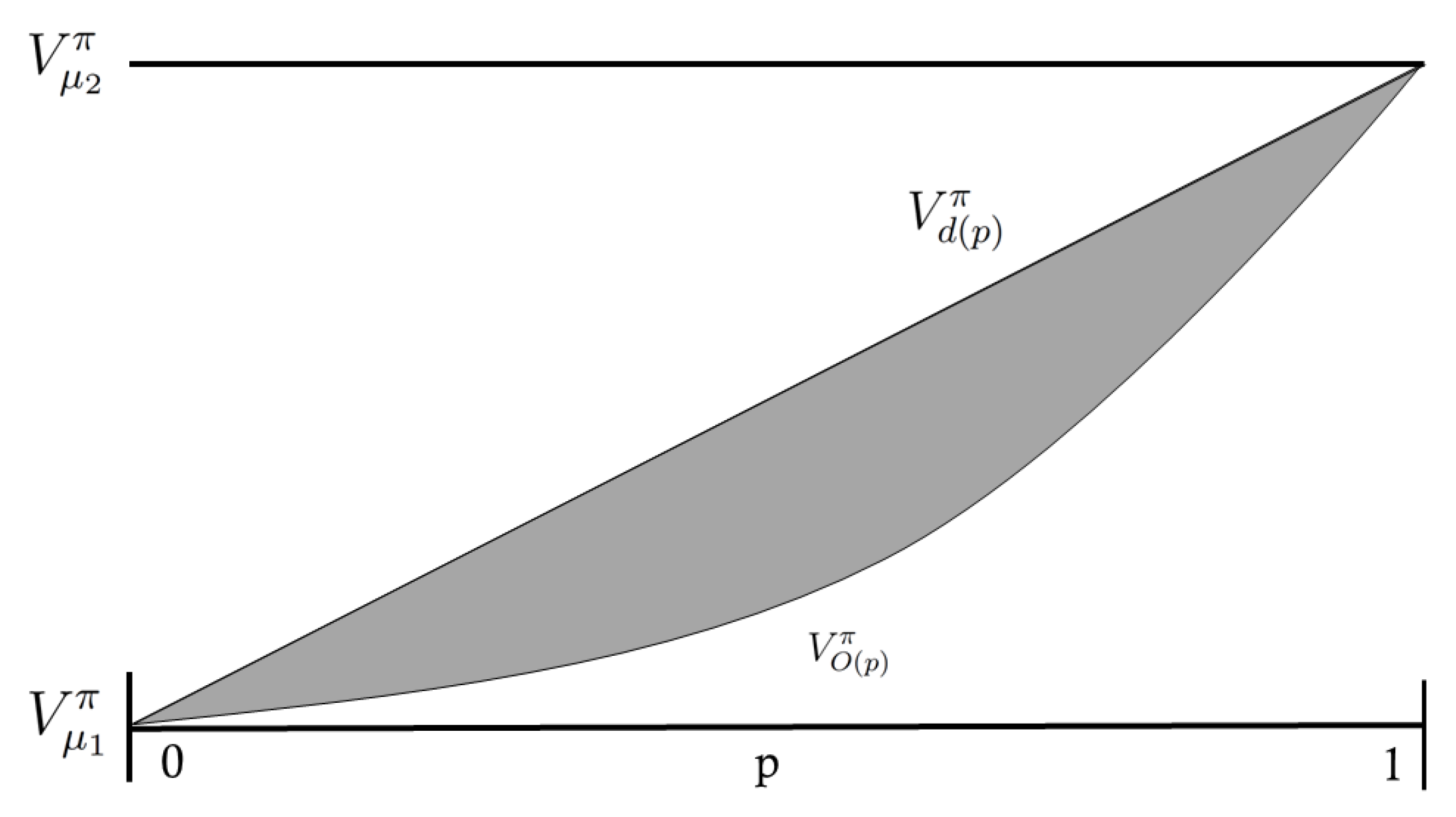
The ideal dissimilarity measure considers the difference in programs along a path generated by a transition function between the two programs. To simulate this transition function, we will merge the two domains. The merging will be performed by taking varying proportions p of two domains and using this as the probability of drawing a sample from the selected domain. So the probability of sampling from the first domain ${\mu }_1$ is $\left(p\right)$ and the probability of sampling from the second domain ${\mu }_2$ is $(1-p)$, where p varies from zero to one. We will assume the path generated by this methodology is the shortest path, but further experimentation will be needed to verify this. We will then use a policy system to traverse the path to generate performance values according to each merged domain. We will similarly use this policy system to generate performances for both domains to plot an expected straight-line average between them. The measure of dissimilarity is defined as the area between the performance curves of the straight-line average for the two domains and their performance combination as a function of mixed amount p. We derive the dissimilarity measure as follows:

$$V_{d\left(p\right)}^{\pi }=V_{{\mu }_1}^{\pi }\ast \left(p\right)+V_{{\mu }_2}^{\pi }\ast (1-p)$$

(7)

$$O\left(p\right)=\{{\mu }_1\left(p\right),{\mu }_2(1-p))\}$$

(8)

$$DS({\mu }_1,{\mu }_2)={\int }_0^1|V_{O\left(p\right)}^{\pi }-V_{d\left(p\right)}^{\pi }|dp$$

(9)

where ${\mu }_1$, ${\mu }_2$ are tests, p specifies a proportion of the two tests, $V_{d\left(p\right)}^{\pi }$ is the proportion of performance of the two tests, $V_{O\left(p\right)}^{\pi }$ is the observed performance of the combined test at proportion p. $V_{\mu }^{\pi }$ is the performance V of the policy system $\pi$ on the domain $\mu$. A pictorial representation of this is shown in Figure 3.

The dissimilarity $DS({\mu }_1,{\mu }_2)$ is the area between the two performance curves O and D for a given agent $\pi$. $O\left(p\right)$ is the observed performance for a given proportion p of the combined test $\{p\left({\mu }_1\right),(1-p)\left({\mu }_2\right)\}$. Similarly, $d\left(p\right)$ is the average performance curve between the two tests for the given performance. When the area between the curves is small, the implication is there is substantial concept overlap between the two domains. When the area between the curves is larger, there is a smaller concept overlap. If the two domains are similar, the area should be close to zero.

Using an AI system within the dissimilarity measure creates a problem with certain combinations of tests. These issues lie within tests that are not mutually exclusive in the concepts needed to solve them. Suppose we have three test suites A, B, and C composed of individual tests $t_n$, where $A=\left\{t_1\right\},B=\left\{t_2\right\},C=\{t_1,t_2\}$. An AI system trained on C would also be capable of solving A. An AI system trained on A would not be capable of solving C without retraining. This produces an effect where the starting point of the AI system can influence the dissimilarity metric. This is undesirable, because a measure of dissimilarity should be symmetric. To address this, it is important to consider merging methods that are not directionally dependent. The method we utilize to address this potential directional problem is to retrain the AI system as it moves along the path between test suites and to use many locations along the path.

The time to compute the distance between all pairs of tests increases quadratically with the number of tests. That is, for n tests in T, the number of distance measurements is $n^2$. This rapid increase is a significant challenge when mapping large test suites into the test space. To combat this problem, we propose a partial mapping of the space. Since the set of intelligence features is finitely bounded, the number of required measurements is also bounded. For instance, if the size of the set is n, we only need to measure any given test in the suite to n others to get its relative position. This optimization was validated through experimentation. The results showed a rapid decrease in error using this approach as the number of tests increases. So, this optimization will be useful and accurate as the number of tests becomes large.

A limitation of our current approach is that the dissimilarity metric is defined through observed agent performance. Therefore, changes in the diversity, capacity, or inductive biases of the agent pool can influence the resulting distances. In this work, we mitigate this issue by using broad and intentionally varied populations, but we acknowledge that a fully agent-independent dissimilarity measure remains an open problem. Developing methods that reduce or normalize this dependence is an important direction for future work on the AIQ framework.

In Section 3.2 we present experiments validating the consistency and accuracy of the dissimilarity measure. Next, we describe how the dissimilarity and complexity measures can be combined into the AIQ measure.

2.6. Artificial Intelligence Quotient (AIQ)

We will now discuss the primary contribution of the work, the Artificial Intelligence Quotient (AIQ). AIQ is meant to exist as a framework for describing and measuring intelligence. We also put forward the AIQ benchmark, which serves as an example of a practical implementation of AIQ and as a means for empirically examining the theory.

2.6.1. Intelligence Space

To examine an AI system’s intelligence, we must examine the domains used to evaluate them. We have previously mentioned combining complexity and dissimilarity into a single measure and will now discuss how this combination can be achieved.

The dissimilarity measure provides us with not only the difference between two domains, but also their distance. As previously discussed, this distance measure can then be used to form a metric space. The resulting space can then be used to represent the distance across unique dimensions of intelligence. The more unique a domain is, the more distant it will be from other domains. The shape’s volume and depth along each dimension indicate the test suite’s effectiveness for evaluating intelligence and whether additional domains are needed to capture the intelligence of a system. This view is from the domain perspective, we will shift it to the agent’s perspective. For an agent to perform well on a test suite of diverse domains, it must be capable of considering several unique concepts. The further the domains are separated in the space; the more concepts are encapsulated in the test suite. From this, the space can be interpreted as not only the domain uniqueness, but also as the space of concepts. We will refer to this space as the intelligence space. An example intelligence space using the CartPole3D benchmark (discussed later) is shown in Figure 1. The dimensionality of the space is reduced to the three most significant dimensions to visualize the space.

While we have constructed this space using only the dissimilarity measure, it is not complete without the complexity measure. Using only the dissimilarity measure results in a space of floating constrained shapes. Each $(n-1)$-polytope formed by applying the dissimilarity measure to a n-sized test suite is neither translationally nor rotationally constrained. To address the problem of translational variance, the test suite must include a fixed and known point in space. This is where the complexity measure proves to be a useful addition to AIQ by capturing the distance between a given domain and the empty test ∅. Therefore, we can add the origin as a fixed and known point.

Adding in the complexity measure fixes the translational issue but has not fixed the rotational issue. The n-polytope formed by this process can still be rotated about the origin using any Euclidean rotation. The number of possible rotational axes can be reduced by including another fixed and known point. A candidate for this point would be the test that is a combination of all other tests. However, we will show the AIQ measure does not need to address either of these rotational variances since it is agnostic to rotation.

2.6.2. Equation Form

While we have described the intelligence space, we will now define the space mathematically. To calculate a given test’s position in space, we will need to measure its distance to every other test. These distance calculations can then be used to create a floating $(n-1)$-polytope. While the number of dimensions this polytope exists in is at most $n-1$ (for an n-sized test suite), there is no reason to assume the polytope will be observed in all $n-1$ dimensions. To ground this shape, we need to measure each test’s complexity value, which creates a distance measurement to the origin. These measurements yield a position in the intelligence space:

$${\mathit{I}}_{\mu }=\hat{s}\left(\mu \right)\times c\left(\mu \right)$$

(10)

where ${\mathit{I}}_{\mu }$ is the location of the domain $\mu$ in n-space. $\hat{s}\left(\mu \right)$ is the unit vector representation of the vector from empty test ∅ to the given test $\mu$ (as defined by its distances from the other domains). $c\left(\mu \right)$ is the complexity of the test $\mu$. The unit vector $\hat{s}$ must be used since the vector s is not normalized. To accurately account for the complexity scalar, we must normalize the position vector; otherwise, the complexity will be disproportionately allocated.

We also need to consider how a given AI system’s performance is included in this measure. We assume an agent’s performance on a given domain can be represented as a single value. This single value can be interpreted as the agent’s ability to perform the tasks in the domain. From this perspective, performance can be treated as a simple scalar multiple to a given domain. Since we only consider domains that halt, we can normalize the performance value to a range of $[0,1]$. The normalization of performance prevents the domain points from being scaled to arbitrary and infinite sizes. This is formalized in the following equation:

$${\mathit{I}}_{\mu }^{\pi }={\mathit{I}}_{\mu }\times V_{\mu }^{\pi }=\hat{s}\left(\mu \right)\times c\left(\mu \right)\times V_{\mu }^{\pi }$$

(11)

where ${\mathit{I}}_{\mu }^{\pi }$ is the performance scaled intelligence point for an agent with policy $\pi$. $V_{\mu }^{\pi }$ is the performance value of the agent’s policy $\pi$ acting on the domain $\mu$. The performance scaled intelligence point is never larger than the unscaled intelligence point $\Vert {\mathit{I}}_{\mu }^{\pi }\Vert \le \Vert {\mathit{I}}_{\mu }\Vert$. Thus, the set of points for the tests in a test suite T executed by agent $\pi$ is defined as follows.

$$T^{\pi }=\forall {\mu }_i\in T,\{{\mathit{I}}_{{\mathit{\mu }}_{\mathbf{0}}}^{\mathit{\pi }},{\mathit{I}}_{{\mathit{\mu }}_{\mathbf{1}}}^{\mathit{\pi }},\dots {\mathit{I}}_{{\mathit{\mu }}_{\mathit{n}}}^{\mathit{\pi }}\}$$

(12)

Referring to the intelligence space in Figure 1 (left), each point in the figure corresponds to a test’s location in the intelligence space. To compute AIQ from these we need to consider how tests are effectively combined. Suppose we have three tests with locations in the intelligence space $A=\{0,1\},B=\{1,0\},C=\{0.5,0\}$. If we combined tests A and B into a suite, we would expect the suite to be $\{A,B\}=\{1,1\}$. If we combined tests B and C we would expect to see $\{B,C\}=\{1,0\}$. This is because test C is a proper subset of test B. From this, we can determine that when we combine tests into a suite, we need to consider the maximized intelligence weights from all sub-tests. This maximization must consider the performance scaled values and not only the test’s location. A low performance scaling can reduce the significance of a domain’s depth in the intelligence space.

To complete the calculation we must restrict what points to consider. In the above example, we would need to compute C but then exclude this point. This effect can be achieved by creating the closed convex subset of positions, which is strictly convex if all boundary points are extreme points [42]. Each point that defines the boundary of the polytope is required to generate the shape and no additional points are included. These points can be determined by computing the convex hull of the set of all points in the suite. These points will need to be calculated after the policy is applied to the domain and not before since the performance scales the resulting point’s position. Suppose we had two identical tests in terms of their complexity and directionality, but a difference in representation. If an AI system achieves a higher performance on one test than the other, this can be attributed to the change in representation and not the agent’s capabilities. So, the higher performance test should be selected over the lower performance test. Creating the closed convex set naturally excludes the lower test. We denote the closed convex subset as

$$T_{min}^{\pi }=hull\left(T^{\pi }\right)$$

(13)

Finally, we can compute the AIQ score from this set of points. AIQ can be expressed as the volume enclosed by these points plus the point generated by the empty test ∅, which is the origin. Since these points generate a polytope (with at most n dimensions) instead of a curved surface, we cannot utilize integration. Instead, we must compute this volume using Gauss’s area formula [43] extended for polytopes [44].

$$AIQ\left(T_{min}^{\pi }\right)={\displaystyle \frac{1}{n!}}\left|\sum _{{\mu }_i\in T}\det (v_1\left({\mathit{I}}_{{\mathit{\mu }}_{\mathit{i}}}^{\mathit{\pi }}\right),\dots ,v_n\left({\mathit{I}}_{{\mathit{\mu }}_{\mathit{i}}}^{\mathit{\pi }}\right))\right|$$

(14)

where $v_i$ are the vertices of the n-polytope. In general, the ordering of the points forming the surface is critical to this calculation. However, since we restrict the shape to be defined by the closed convex set, we can ignore the ordering because every set ordering results in the same value. The exact calculation can prove computationally expensive, so approximations to the exact measure are normally preferable. An example of the scaled n-polytope generated for the CartPole3D benchmark with an AI system is shown in Figure 1 (right).

2.6.3. AIQ as a Benchmark

While the AIQ score is defined theoretically, a practical implementation is needed to evaluate the theory and measure an AI system’s intelligence. The AIQ benchmark is an initial test suite that demonstrates a practical implementation of the framework.

The domains included in the test suite are MNIST [45], FMNIST [46], CIFAR10, CIFAR100 [47], CartPole2D [48], and CartPole3D [14]. The first four domains are classic image classification domains. The last two domains are control problems typically used with reinforcement learning systems. While most of these tasks are trivial for modern AI systems, these domains were selected due to an intuitive understanding of how similar and complex they are to each other. Since the CartPole domains are time series based, a reduction is needed to evaluate them. We create an effective AI system capable of achieving consistently high scores in the domains. This system is then utilized to create a large set of observation-action pairings. The pairings are then mapped onto a similar structural representation as the other classification domains.

While we utilize a reduction in the CartPole domains for this initial AIQ benchmark, it is not necessary in general. An alternative solution would utilize a differing set of calibration AI systems. Some systems offer multi-task capabilities that could prove effective in performing a more robust calibration, such as the Gato system [49]. Another approach is to use a set of AI systems and find methods for combining tests within AIQ even when their calibration methods differ across domains. This is beyond the scope of this work and will be reserved for future study.

So far, we have only considered a single performance scaling value in our evaluations. This value is whatever the domain returns, in this case it is the mean categorical accuracy. Other metrics may provide further insight. The speed of the AI system’s solution could also be used as a scaling measure, where faster results are given better scores. This idea is addressed in depth by [29]. Other measures such as memory consumption, steps to get to the solution state, and minimized agent size could also be utilized.

3. Results

In this section, we present experimental results validating the accuracy and consistency of the complexity, dissimilarity, and AIQ measures. We introduce a new CartPole3D domain for evaluating AI agents’ ability to handle open-world novelty and as a basis of an new AIQ benchmark. When then show the results of using this AIQ benchmark to measure the intelligence of four independently-created AI systems.

3.1. Complexity Results

This section evaluates the MCCP complexity measure through several experiments. We compare it with information-theoretic baselines, examine its behavior on tasks with intuitive difficulty orderings, and assess its sensitivity to population sampling. We further demonstrate its practical value through an applied domain-analysis example.

Since the MCCP measure is defined theoretically, several practical approximations are required to implement it. First is the choice of a generalizable policy class. While no truly general-purpose policy exists, some approximations have been proposed [50]. In line with current practice in AI research, we treat neural networks as the most broadly applicable class of policies and use them as our operational proxy for a generalizable AI system.

The second approximation involves evaluating policies across the entire spectrum of performance values, which is typically infeasible. To address this, we generate a random population of neural-network-based agents. Their capacities vary according to their trainable parameters, which are determined by randomly sampled node counts and layer widths. Each agent is trained for an identical number of epochs, and its resulting performance is recorded. These capability-performance observations are then used to fit a linear estimator relating parameter count to achievable performance. The estimator provides approximate performance values in regions where no agent was observed, producing a piecewise-defined capability-performance curve.

We compute the area under this curve (AuC) across the observed performance range as an empirical approximation of the MCCP complexity. To enable cross-domain comparisons, the AuC values are normalized.

3.1.1. Domains

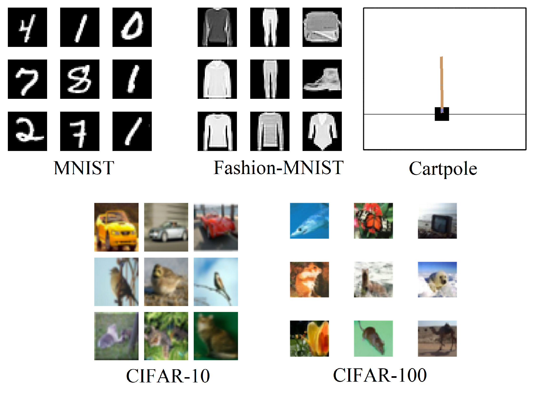
For these experiments, we focus on five well-established domains. Four are image datasets (MNIST [51], Fashion-MNIST [46], CIFAR10, and CIFAR100 [47]), each of which we convert to greyscale to simplify computation. The fifth domain is the CartPole reinforcement learning task [52]. These datasets are illustrated in Figure 4. To evaluate all domains using a consistent methodology, we convert CartPole into an image classification task by running a trained agent and collecting image–action pairs. This allows us to apply the same complexity measurement procedures across all domains. Although our measure is applicable to reinforcement-learning environments, standardizing all domains as classification tasks avoids representational discrepancies within the test suite. When CartPole is analyzed in isolation (Section 3.1.4), we instead use its native sensor-based observation vectors, as representational bias relative to other domains is no longer a concern.

3.1.2. Entropic Verification

As noted earlier, one classical way to estimate task complexity is through Kolmogorov complexity. Because Kolmogorov complexity is not computable in practice, various approximations are commonly used. One such approximation is Shannon entropy [53].

For image datasets, we define the Shannon entropy as the average local entropy computed for each pixel within a fixed neighborhood. In our experiments, we use a radius of one pixel, which typically corresponds to a locality of five pixels, with smaller neighborhoods occurring at image boundaries. The entropy of each locality is computed as the minimum number of bits required to encode it. Since this calculation does not include label information, we incorporate the labels by adding ${log}_{2}C$, where C is the number of classes in the dataset. For example, CIFAR100 has 100 classes, so we add 3.32 bits to the average locality entropy of each image. Summing these values across all images yields the dataset’s total entropy.

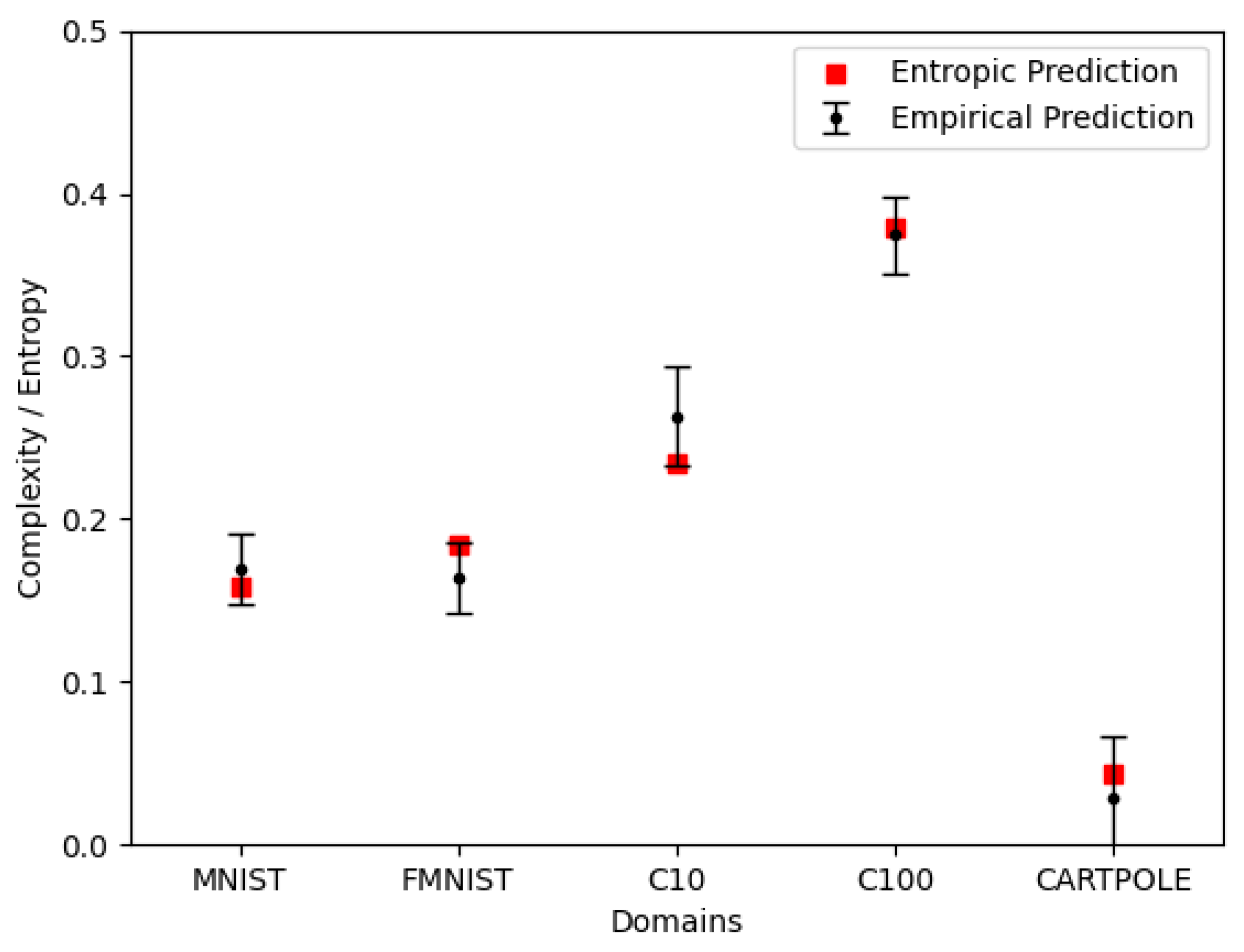
In this experiment, we compute the Shannon entropy for several well-known datasets and compare these values to the MCCP complexity measure. We normalize the resulting entropy values across datasets for direct comparison; we refer to these normalized values as entropic predictions.

We compare the normalized entropic predictions with the normalized MCCP values, as shown in Figure 5. The MCCP measure behaves as expected: the domains are ranked intuitively, with CIFAR100 exhibiting the greatest complexity and CartPole the least. Moreover, the MCCP estimates closely track the entropic predictions, remaining within the 95% confidence intervals. Because entropy is closely related to Kolmogorov complexity, a well-established indicator of inherent task difficulty, these results support the use of MCCP as an effective measure of domain complexity.

3.1.3. Known Difficulty Verification

Another way to validate the MCCP complexity measure is to apply it to tasks whose relative difficulty is already known. A natural approach is to take a dataset with many classes and evaluate how complexity changes as the number of classes increases. If MCCP rises in accordance with this increase, the measure is behaving correctly.

For this experiment, we use the CIFAR100 dataset. We create subsets by selecting groups of ten classes—for example, a 10-class subset uses classes 1–10, a 20-class subset uses classes 1-20, and so on. We then compute the MCCP complexity for each subset, using 100 randomly generated agents for each measurement.

The results, shown in Figure 6, exhibit a clear nonlinear increase in complexity as the number of classes grows, which is expected. Once the task becomes sufficiently challenging, adding additional classes yields diminishing increases in difficulty. These findings confirm that MCCP successfully ranks the CIFAR subsets in accordance with their known relative difficulty.

3.1.4. Parameter Analysis

This experiment evaluates how the MCCP complexity measure can be used to compare the complexity of two domains, and how changes to a specific domain parameter influence that complexity.

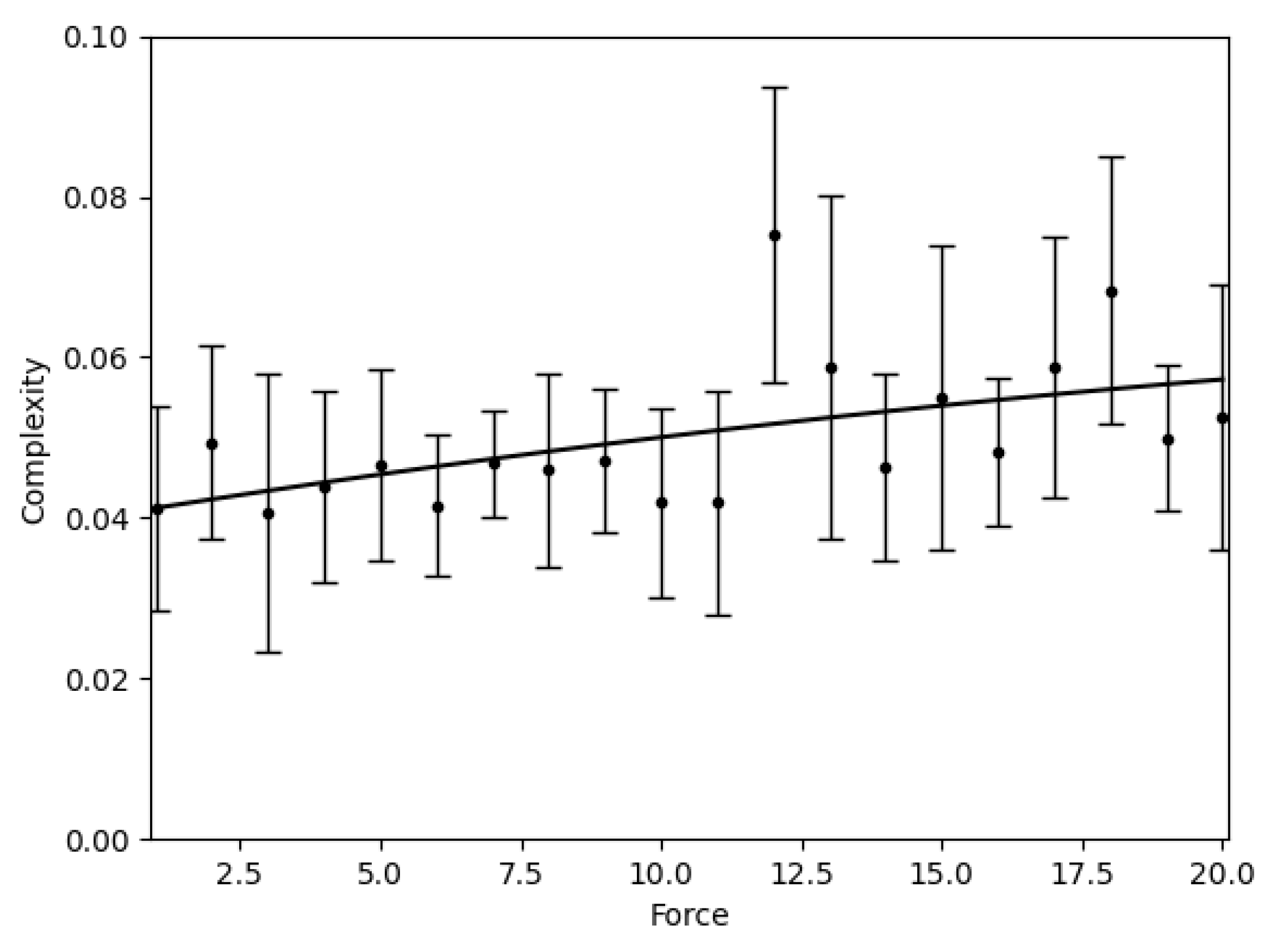
For this experiment we utilize the CartPole domain. For each change to the domain, we alter the force applied to the cart for each action (push left or push right). The value is normally fixed to 10.0. In our experiment we vary the value between 1.0 and 20.0 in 1.0 intervals. The resulting complexity was measured for each new force variation. Each measurement uses 15 samples from the pool of agents. The error bars are the 95% confidence interval for our measurement.

Figure 7 presents the results of this experiment. The data show a clear positive correlation between applied force and measured complexity. This trend aligns with intuition: in CartPole, greater force amplifies the risk of over-correction, making the task increasingly difficult. Across our trials, we did not observe force values that were too small to maintain balance in most runs.

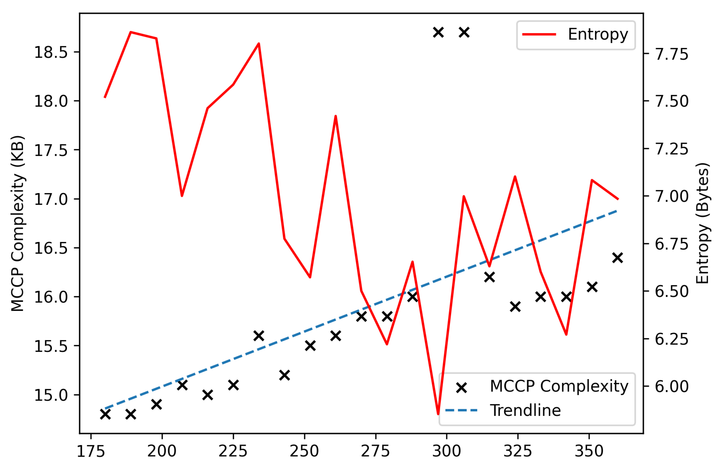
As a second experiment for analyzing a parametric shift, we vary the gravity in the CartPole domain. The gravity affecting the CartPole was varied from 180 to 360 in steps of 9, from its normal gravity of 9.8. Prior work has indicated a clear performance drop as gravity is increased [54], but only for gravity values higher than 180. This performance drop will serve as the basis for our assumption of an increase in the complexity.

The entropy of the domain is calculated by examining the state of the domain. A trained agent is run on the domain and a list of domain observations (Cart Position, Cart Velocity, Pole Angle, Pole Angular Velocity) is compiled for 100 episodes. The data is stored in discretized values by creating 30 evenly distributed bins over the range of observed values for the domain value. The probability distribution is then measured for each value in the domain observation. The entropy is then computed for each of the four distributions and summed. The concept behind this is that a more sporadic set of observations implies a greater variance in the data and thus a more complex domain.

The agent architectures used in this experiment were randomly selected from a pool of 1 to 3 layers and 1 to 32 nodes. The agents were trained using a DQN system with a maximum of 10M steps. The training process was halted upon convergence.

The results of this experiment are shown in Figure 8 and indicate a clear increase as the gravity of the domain is increased. While the trendline indicates a linear relation, we believe this is best represented by the start of a logarithmic relation. The gravitational increase should tend towards an impossibly challenging domain. This would result in the convergence of the MCCP complexity value once the gravity is sufficiently high. The two outliers at 300 are the result of an overly large network being observed as the minimum network to achieve higher performance results, which can be addressed with additional network agent sampling.

The entropy of the domain shows a high variance for the domain, even after sampling 100 episodes. A trend is still observable in the results and indicates a decrease in the entropy as the gravity of the domain increases. This indicates the variance of the domain is inversely related to gravity. The inverse relation suggests that using entropy as a measure of domain complexity may not create accurate results. Variance alone may not be a sufficient indicator of domain complexity. Therefore, MCCP is superior to entropy for measuring the complexity of an AI domain.

3.1.5. MNIST Noise

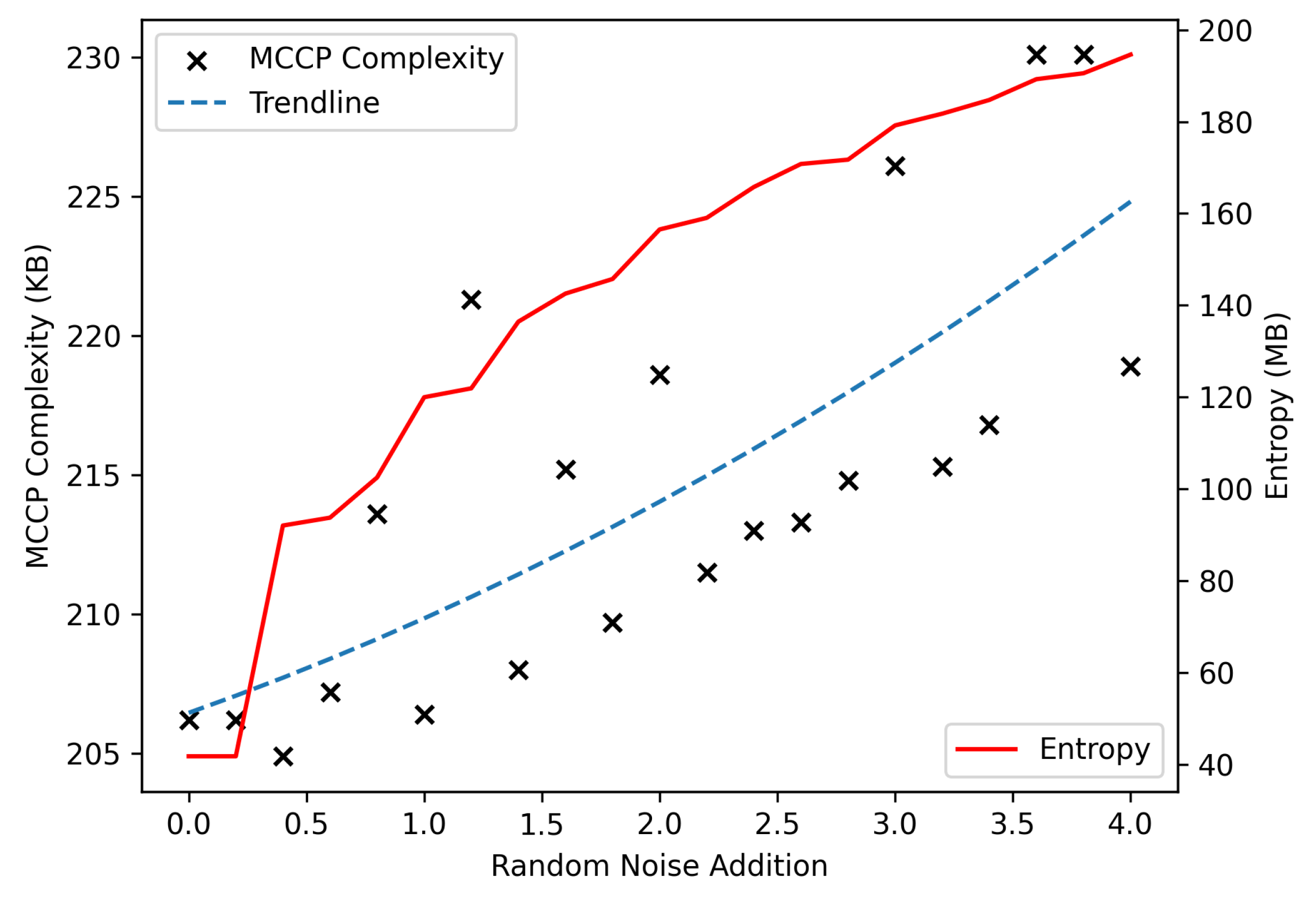
Another method to increase difficulty is to increase the noise of a given domain. To effectuate this, we will begin with the image classification domain MNIST [45]. We will then add an increasing amount of noise to each image. The entropy of the domain is calculated by taking the sum of the entropy of the 2D images (in greyscale) plus the entropy of the labels associated with each image. The agent pool for the MCCP complexity measure were randomly-constructed networks with a (32 × 32) input, 1–2 convolutional layers containing 1–32 nodes with 3 × 3 kernels, and a 2 × 2 max-pool layer. The network ended with a fully connected layer of 100 nodes.

The results from this experiment are shown in Figure 9 and indicate a linear increase in the MCCP complexity measure as a function of the noise increase. A logarithmic increase in entropy can be observed. This is due to the increasing random noise resulting in a decrease in the signal to noise ratio. As the signal to noise ratio decreases, the entropy of the domain will eventually plateau to a fixed constant. MCCP complexity outliers can be observed in the data. This is due to not observing smaller policy systems where they would have been sufficient to achieve the same performance value as the larger observed system. These outlying points can be corrected by increasing the number of samples or utilizing the same set of randomly generated policies between MCCP complexity measurements.

The results of the entropy measure on this domain are like those seen in the previous experiment. This is because the complexity variation of the two domains is the same. The complexity variation is a function of the noise/variation being added. From this we can determine that the introduction of variance into the two domains is consistent and effective. We see the MCCP complexity measures differ in these domains. This is due to the MNIST domain being very stable. A large amount of noise added to the domain has a minor effect on the accuracy. Once enough noise is added, the accuracy declines rapidly requiring a more complex policy agent to achieve equivalent performance.

3.1.6. MNIST Duplication

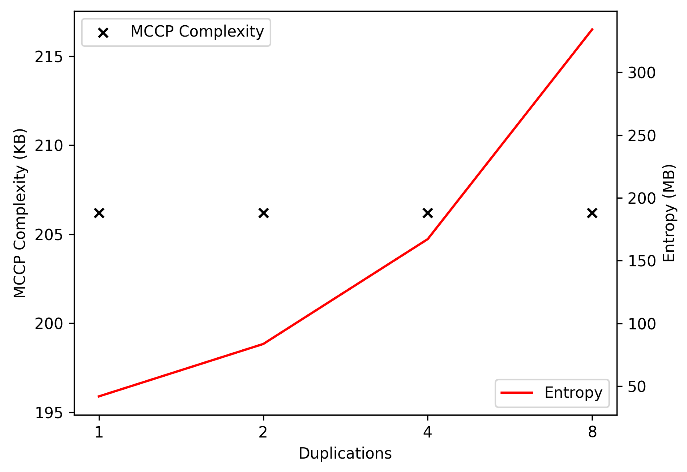
While we have previously examined methods to intuitively increase the complexity of domain, in this experiment we will instead focus on keeping complexity constant. To achieve this we will use the MNIST domain as a base and append onto it the same 50,000 base images onto itself. The number of classes will remain the same and the number of images will increase by 50,000 for each duplication. The duplication is consistent across train and test sets. While the domain is increasing in size, the complexity should remain constant as no additional information is being added.

The results of this experiment are presented in Figure 10. A constant value for the MCCP complexity measure is observed as the number of duplications increases. For the entropy, the resulting measure scales proportionally to the number of duplications used. From this, we can determine that the MCCP complexity measure is consistent with the constant complexity of the domain while the entropy measure is not. This divergence indicates that simply examining the compressibility of the domain is inadequate for determining the complexity of the domain.

3.2. Dissimilarity Results

In this section, we evaluate the dissimilarity measure through a series of experiments. We apply the measure to domains with intuitive differences to verify that it behaves as expected, using the same set of domains employed in the complexity analysis (see Section 3.1.1). The results show that domains with known relative dissimilarity are accurately and consistently ranked. We also present a practical example illustrating how the measure can support test suite analysis.

3.2.1. Zero Distance

One obvious test is whether a given domain’s distance to itself is zero. While the equation has been shown to generate this result in general, a practical implementation might yield differing results. To examine this behavior, we measure the dissimilarity between the MNIST domain and itself, ${\mu }_1={\mu }_2=\mathrm{MNIST}$. This was done by selecting eleven evenly-spaced proportion values from zero to one in increments of 0.1. We then trained the system on mixtures of the two domains according to the proportion, but each mixture ends up being an exact copy of the original domain. The results for this experiment can be seen in Figure 11.

While the results look sporadic, the dissimilarity is actually low between the domain and itself. The performance difference between the domain and itself is only 0.0006. The non-zero performance difference is likely a result of experimental variation, such as randomly assigned initial network weights for an AI system. The resulting dissimilarity between MNIST and itself is measured at $1.7\times {10}^{-4}$.

3.2.2. Different, but Similar Domains

It is important to examine the dissimilarity measure on domains that share several similar concepts but whose actual content differs significantly. For this we will calculate the dissimilarity between the two domains MNIST and CIFAR10. These two domains share very little content; however, the same methodology can generally be used to effectively solve both domains.

The results for this experiment are shown in Figure 12. We observe a dissimilarity of $0.018$ between the two domains. This indicates that while the domains may not share any content, they are still very closely related to each other.

3.2.3. Subset Distance

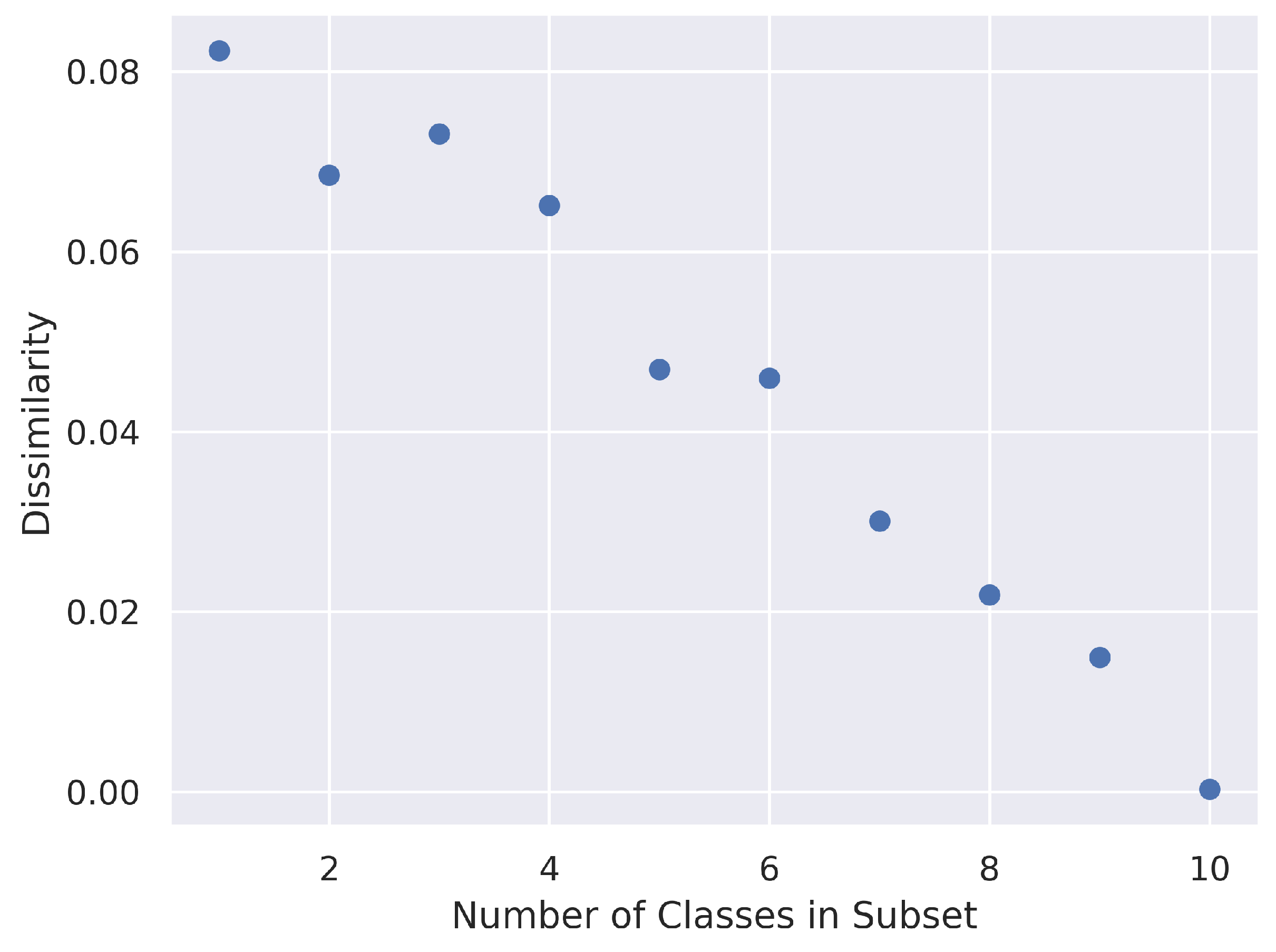
Next, we evaluate how dissimilarity measures the distance between domains with a known difference. One approach is to use the known difference between a subset of the domain and the full domain. An increasing difference should be observed if we remove classes from the full domain and then compare to the full domain. We use domain CIFAR10 and split its classes into subdomains. We generated 10 subdomains based on the number of classes (i.e., CIFAR-N = classes $\{0,\dots ,n\}$ from CIFAR10). We then measured the dissimilarity between the subdomains and CIFAR10. Results are shown in Figure 13.

There is a clear linear trend in proportion to the number of subclasses utilized in the subdomain and the resulting dissimilarity from the CIFAR10 domain. This indicates that the dissimilarity measure is capturing the known difference decrease as expected. Since the dissimilarity measure is bounded, we would eventually expect to see a curved trend as the number of classes increases. This would be due to not every class being mutually exclusive to each other. Since CIFAR10 is relatively small, we have not yet observed any class overlapping.

3.2.4. Known Parametric Shift

If a domain experiences an observable parametric shift, we would expect the dissimilarity to increase in response. In this experiment we compare a parameter shift in the CartPole domain. We modify the environmental gravity from its original 9.8 to the range of [0, 200] in increments of 20. We then use the dissimilarity measure to compare all combinations of gravity variations. This process generates a cross table of resulting dissimilarity values which is illustrated using a heatmap in Figure 14.

We observe a clear increase in dissimilarity as the parametric difference between the two domains increases. The resulting R-value between dissimilarity and parameter difference is 0.70, indicating a strong positive correlation between the dissimilarity measure and parametric differential. This supports the notion that the dissimilarity measure is effectively capturing a change between domains, even when the exact change may not be directly visible. The resulting data indicates a symmetry about the diagonal. This indicates that the dissimilarity measure works in both directions of the parametric shift and generates a repeatable result. This would not be the case for the MCCP complexity measure due to the fact that training on high-gravity environments is sufficient to handle low-gravity environments, but the opposite is not true.

3.3. AIQ Results

We present several experiments to validate that the measures and framework can consistently and effectively measure the intelligence of AI systems. We will first compare the complexity measure and the dissimilarity measure to show that both are measuring the correct property of the intelligence space. We will then create the AIQ benchmark using a test suite measured with the AIQ framework. We will then show how the AIQ score of a system with a known decrease in capacitance compares to the system’s average performance. We will use the same domains described earlier in Section 3.1.1 plus a new domain, CartPole3D, which is described later in Section 3.4.1.

3.3.1. Complexity vs. Dissimilarity

Given that we have two unique measures for Complexity and Dissimilarity, it could be presumed that they are both measuring differing ideas. However, since the space of intelligence is constructed from these two measurements, there is significant overlap. Suppose we had two domains, A and B, that varied in complexity but shared the same directionality in the intelligence space. In this case, $\widehat{{\mathbf{i}}_A}=\widehat{{\mathbf{i}}_B}$ and $|{\mathbf{i}}_A|\ne |{\mathbf{i}}_B|$. We would then suppose that the difference in complexity between the two domains would be equivalent to their dissimilarity.

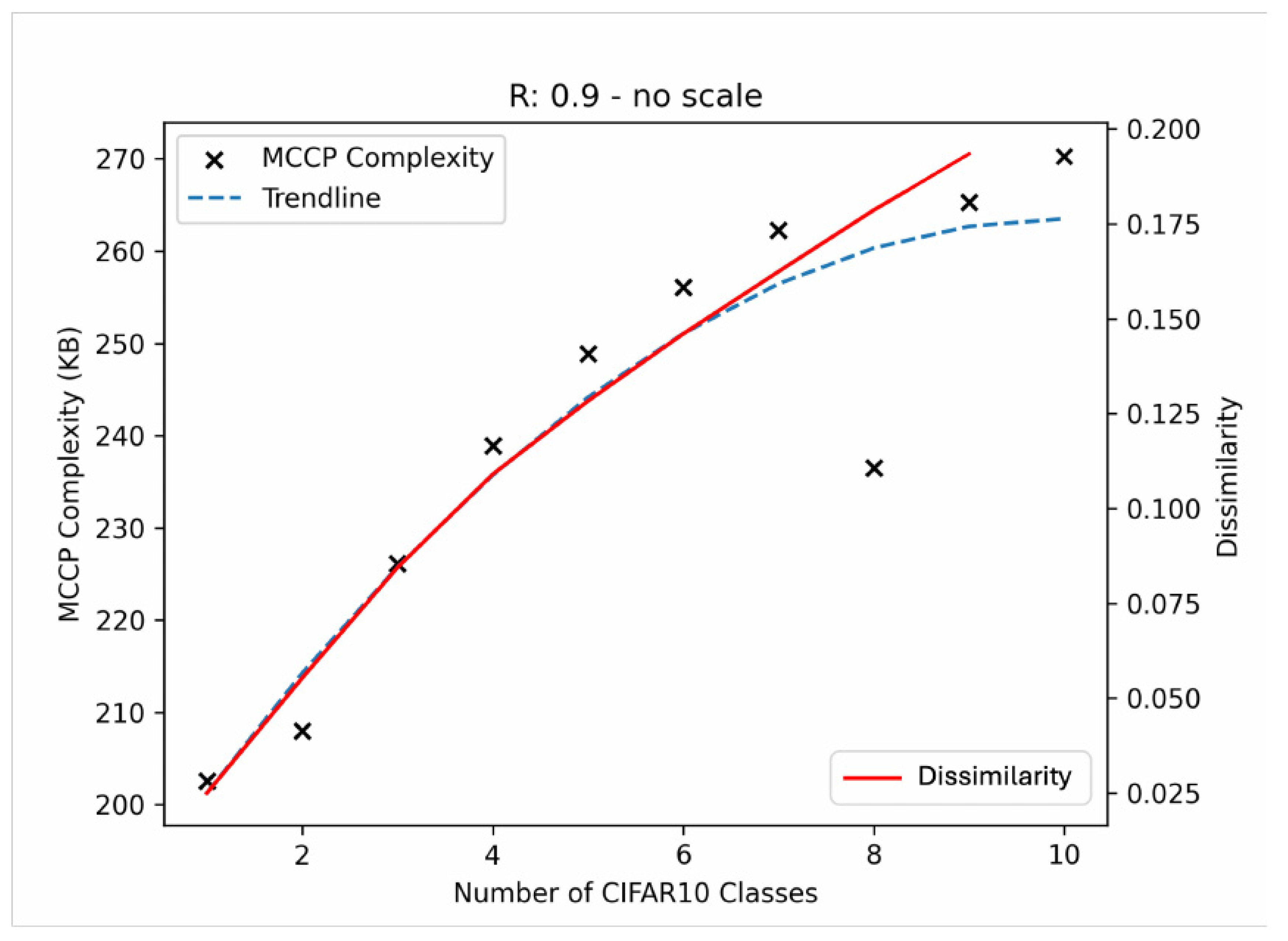
To evaluate this expected behavior, we will utilize the CIFAR10 domain. We will then use its classes as the basis for these differing domains (e.g., class $\left\{1\right\}$ will be A and classes $\{1,2\}$ will be B). Since the subsets are used as the difference between domains, we can assert that the domains will have a varying complexity and the directionality of the domains is the same. This assertion may not hold for larger domains due to them potentially encapsulating several differing concepts, but CIFAR10 and its subsets should be small enough to not notice this behavior. We compare the MCCP complexity of each subset of the CIFAR domain (e.g., $C\left(A\right),C\left(B\right),\dots$) and dissimilarity between each subset in CIFAR10 (e.g., $DS(A,B),DS(B,C),\dots$). The results are shown in Figure 15.

The results show a significant correlation (R-value = 0.9) between the MCCP Complexity and the Dissimilarity. We can see that the dissimilarity does deviate from the MCCP Complexity towards the end. This could be due to the scope of concepts in the CIFAR10 domain increasing over the number of subsets used. It could also be due to the intelligence space being non-Euclidean in nature. If the directionality of the domain is not aligned with an axis in the space, we would see a non-linear growth in one dimension causing a deviation from complexity. This experiment shows that complexity and dissimilarity measure the same concept in the intelligence space when the domains have the same directionality and differing complexity. This indicates that our representation of the intelligence space is coherent.

3.3.2. AIQ Benchmark Complexity

To construct the AIQ benchmark, we will need to measure the test suite’s complexity. We utilize the MCCP Complexity measure to determine each of the domain’s complexity. Since each domain has similar inputs and outputs, we will utilize the same pool of randomly generated architectures for each. Using the same pool should reduce potential minimization bias in architecture selection. The results are shown in Figure 16.

The results are consistent with previously conducted experiments. The NIST problems are in a similar group followed by CIFAR10 and CIFAR100. CartPole2D is also observed to be a less complex domain than its higher dimensional counterpart CartPole3D. A large base complexity value is observed in each domain. This is due to the large size of the smallest domain observed in each measurement. One method to address this is to reduce the number of inputs and outputs to the network. This was not done to prevent a potential bias due to using dimensionality reduction, but may be useful in future work.

3.3.3. AIQ Benchmark Dissimilarity

The dissimilarity between domains must also be determined before computing AIQ scores. This experiment will utilize the dissimilarity measure. We will create evenly spaced mixtures of each combination of domains and compare their combined performance on a suitable agent to the diagonal between their respective single domain performance values.

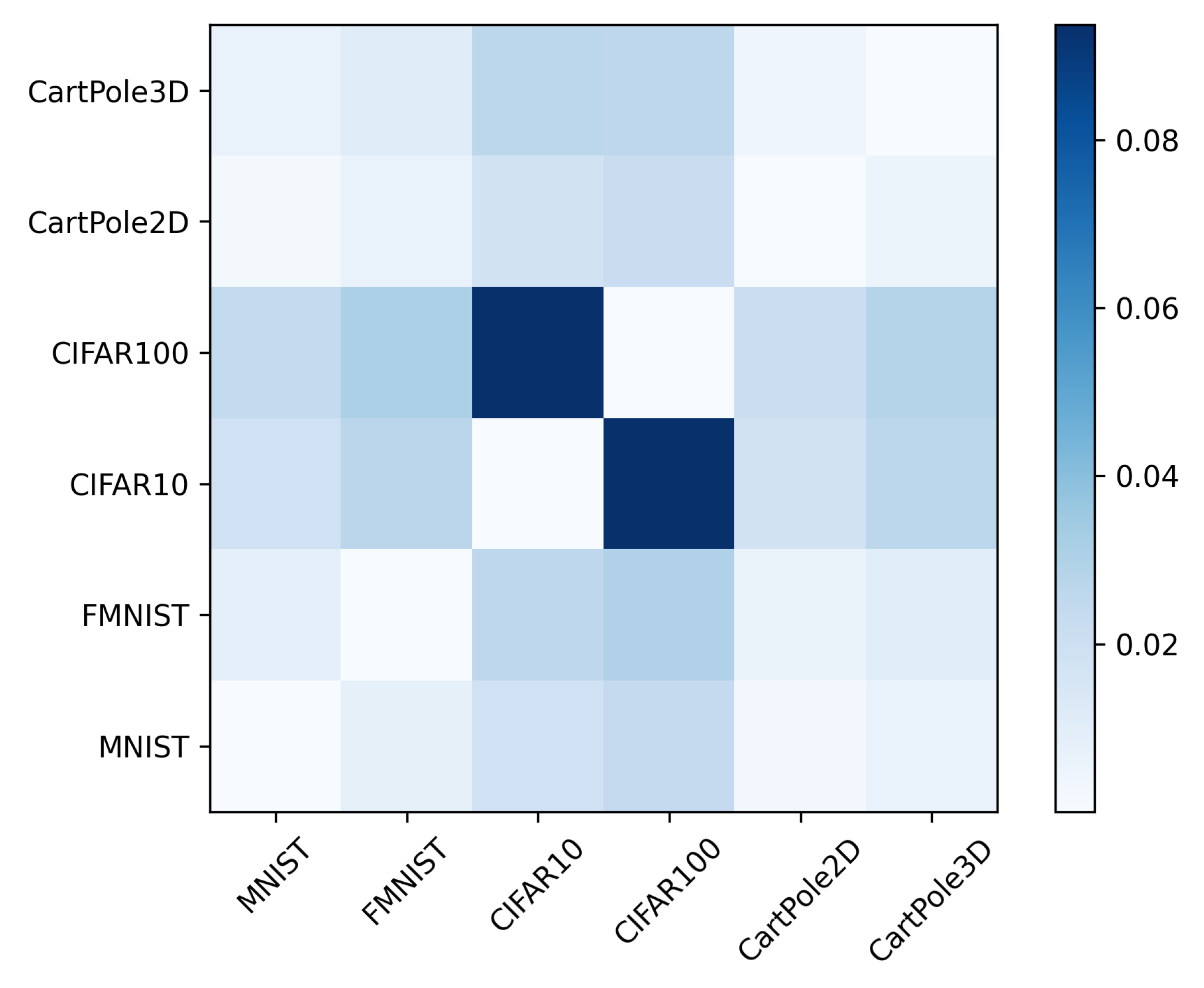
The results in Figure 17 show a clear low dissimilarity value across the diagonal, indicating each domain is similar to itself. We can also observe the similar domains are correctly grouped. The NIST domains are similar to each other and the CartPole domains are similar to each other. The CIFAR domains are still dissimilar due to CIFAR100 involving many more classes than CIFAR10.

The results in Figure 17 also show that adding another subtest to the combined test will not significantly change the results. This is due to the similarity measure accurately capturing a near zero distance between any two identical domains. This shows that the framework can be used to generalize testing to include more sub-tests that can further measure the general intelligence of a system without biasing the benchmark by adding many similar tests.

3.3.4. AIQ Benchmark Complexity vs. Dissimilarity

We computed the absolute difference in the MCCP Complexity between the domains in the AIQ test suite, shown in Figure 18. These values do not resemble those in the dissimilarity heatmap shown in Figure 17. The dot product similarity between the two datasets is 0.24, indicating a weak correlation. This demonstrates that complexity and dissimilarity are different when measuring domains that are not changing along a single dimension of intelligence.

3.3.5. AIQ Benchmark Intelligence

We will now construct the dimensions of intelligence being utilized within the AIQ benchmark. To reiterate the procedure, we begin by taking dissimilarity values between every domain and normalizing them. The normalized dissimilarity values are then be used in the multilateration process assuming the empty test as a fixed point at the origin. The resulting points are then multiplied by their respective complexity values to generate the domain’s location in the intelligence space. In this experiment, we chose not to remove unnecessary dimensions of intelligence because the multilateration process did not produce extraneous dimensions.

The results in Figure 19 show that the MNIST, FMNIST, and CIFAR10 domains are strongly capturing the fifth dimension of intelligence. The more complex domains of CIFAR100 and CartPole3D are capturing the fourth dimension of intelligence. CartPole2D and CIFAR10 are only weakly capturing the third dimension of intelligence. From this, the AIQ benchmark appears to only be capturing approximately two dimensions of intelligence. A more diverse test suite would encapsulate more dimensions of intelligence.

3.3.6. AIQ Handicapping

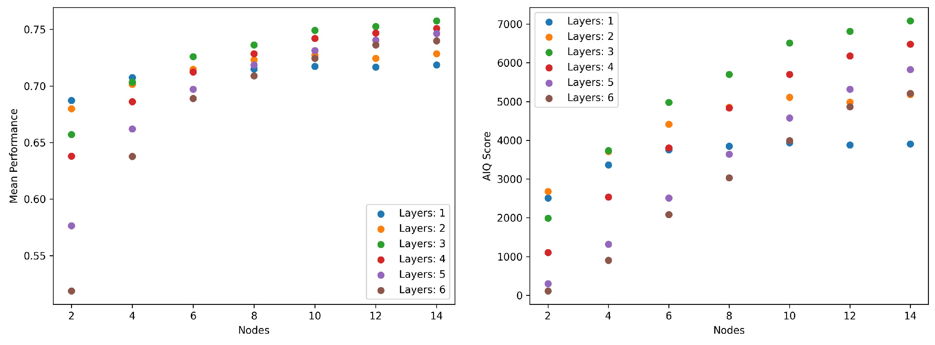
We will now validate whether the AIQ benchmark is evaluating the intelligence of an AI system. We begin with a large network of fully connected nodes and “handicap” the system by removing nodes. This process is repeated with a variable number of layers in each AI system. The nodes and layers are treated as separate variables as either may have more or less impact depending on the number of parameters in the agent. We also measure the simple mean performance of the AI systems and compare it to the AIQ score.

The results are shown in Figure 20. From the mean performance plot, we can see a clear increase in performance as the number of nodes increases until convergence is reached. This effect is not fully observed when using the AIQ score, as the agents with one layer show a decrease as the number of nodes increases beyond a point. We also zoom in on the data until convergence is reached, from 0 to 14 nodes, in Figure 21. When only considering the smaller range of nodes, we can more clearly observe a differing trend between the AIQ score of the agents and their mean performance. The AIQ score is more linearly related to the change in nodes than the corresponding mean performance which is more quadratically related to the change in nodes. This indicates that the AIQ score is measuring the capacitance of the AI systems better than the mean performance.

3.4. Application to Open-World Novelty

In this section, we illustrate how the complexity, dissimilarity, and AIQ measures can be applied to evaluate novelty within domains and to assess the intelligence of AI systems designed to adapt to such novelty. DARPA’s Science of AI and Learning for Open-world Novelty (SAIL-ON) program [55,56] was created to advance methods for detecting, characterizing, and accommodating novelty. As part of SAIL-ON, our team at Washington State University (WSU) developed novelty generators to evaluate how well AI systems handle open-world novelty. We constructed generators for three distinct domains: CartPole3D, activity recognition in smart environments [57], and the VizDoom first-person shooter game [58]. For each domain, we designed multiple novelty types that were complex enough to challenge the agents and dissimilar enough to evaluate the AI systems across multiple dimensions of intelligent capabilities.

The SAIL-ON program designed several metrics for evaluating an AI system’s ability to detect and accommodate novelty. However, the AIQ measure, using the different novelties as a test suite, compares the AI systems based on more than novelty handling. The systems can be compared based on the capabilities that allow them to perform well with or without novelty. In this section we focus our analysis on the CartPole3D domain, because we were able to evaluate the novelty generator on four different AI systems designed by other institutions. The VizDoom domain was attempted by two institutions, and the smart environment domain by only one. More information about all three domains and the novelty generator can be found at https://github.com/holderlb/WSU-SAILON-NG (accessed on 25 November 2025).

3.4.1. CartPole3D Domain

To better aid in measuring an AI system’s detection and adaptability to sudden domain shifts, we developed the new domain CartPole3D. See Figure 22 for a visual of CartPole3D. This domain is a recreation and extension of the classic CartPole control problem [48]. There are a few significant differences between CartPole3D and CartPole. First, CartPole3D is implemented in three dimensions. This additional dimension allows for a more challenging control problem and allows agents more interaction in the domain. To do this, we utilized the realistic physics simulation PyBullet [59]. This additional dimension doubles the action space available to the AI system. The available actions are to push the cart right, left, forward, backward, or do nothing. The directional actions apply force to the cart in a constant direction (regardless of where the cart is facing). The nothing action has no effect on the CartPole and only progresses the domain in time.

The second change is the addition of balls to the domain, which allows for more interactions to happen in the environment than if only the cart and pole were present. The balls normally move straight and bounce when hitting another object and ignore the gravity of the domain.

CartPole3D runs for a maximum of 200 ticks or until the pole falls over, i.e., exceeds 12 radians from vertical in any direction. Unlike CartPole, CartPole3D does not terminate when a certain position in space is reached. However, all objects are constrained to a $10m$ cube. The cart is positioned at the bottom of this cube and is only allowed to travel in that plane. Performance is calculated as t/200, where t is the number of ticks that the pole remains balanced. At each tick, the agent observes the cart’s position ($x,y$) and velocity ($v_x,v_y$), the pole’s position (${\theta }_{yaw},{\theta }_{pitch},{\theta }_{roll}$) and angular velocity ($v_{yaw},v_{pitch},v_{roll}$), and each ball’s position ($x,y,z$) and velocity ($v_x,v_y,v_z$).

With this new domain we can evaluate a larger breadth of domain shifts than were possible with the simpler CartPole2D domain. To effectuate this, we implemented 16 types of sudden domain shifts (see

Table 1. CartPole3D Novelty Implementations.

Novelty Level	Effect
0	No change.
1	Change to mass of cart.
2	Block is unmovable in plane of cart.
3	Blocks initially pushed towards random point.
4	Change in size of block.
5	Blocks pushed away from each other.
6	Gravity increased and does affect blocks.
7	Blocks attracted to origin.
8	Additional stopped blocks spawned over time.
9	Cartpole pole length increase.
10	Blocks move on fixed axis in plane of cartpole.
11	Blocks initially pushed towards cartpole.
12	Increase bounciness of blocks.
13	Blocks attracted to each other.
14	Wind force applied.
15	Blocks pushed towards pole tip.
16	Additional blocks spawned over time.

). A domain shift is a single parametric change (ideally irreducible) in the domain. This change is further partitioned by difficulty into easy, medium and hard categories. For example, the change in the mass of the cart in novelty type 1 is further divided into small, medium and large changes in the cart mass. To evaluate the AI systems on novel domain shifts, we kept the changes in the domain hidden from the AI system developers.

3.4.2. SAIL-ON Metrics

The DARPA SAIL-ON program [55] developed several metrics to capture the different aspects of performance. For the AIQ benchmark we will focus on just one of those metrics, the Asymptotic Performance Task Improvement (APTI). APTI compares the performance of the AI system $P_{\alpha }$ to that of a baseline system $P_{\beta }$ near the end of a trial consisting of multiple attempts at the CartPole3D task. Specifically, $APTI=P_{\alpha }/(P_{\alpha }+P_{\beta })$. The better the AI system performs relative to a non-novelty-aware baseline system, the higher its APTI.

3.4.3. CartPole3D AI Systems

The evaluation is conducted on four CartPole3D agents from four different institutions: Australian National University (ANU), University of Colorado at Colorado Springs (UCCS), Palo Alto Research Center (PARC), and University of Massachusetts Amherst (UMass). We describe each system briefly below, but a detailed description is beyond the scope of this article. These agents were compared against our own baseline agent. The novelties were hidden from the external teams until after their agents were designed and evaluated.

The baseline state-of-the-art (SOTA) AI system is a DQN neural network with two fully-connected layers of 512 ReLUs, with an input size of 10 and 5 outputs. A single option is selected from the 5 outputs, resulting in a single domain action per step. The baseline AI system was trained for a fixed number of 500,000 steps using Boltzmann exploration. To better achieve convergence, the ball information is not sent to the baseline. While this does decrease the maximum potential performance, it stabilizes results. The SOTA agent is not novelty aware, so performance will decrease when novelty is introduced.

The method used by ANU’s agent is called NAPPING for Novelty Adaptation Principles [60]. NAPPING is not an AI agent itself, but a novelty adaptation module that is attached to an existing agent of the domain. In the case of Cartpole3D, we use the existing baseline agent described above and add ANU’s module to it. ANU’s module observes the performance of the baseline agent, and as soon as a drop in performance is noticed, ANU’s module begins to adjust the actions selected by the underlying agent. The pre-novelty performance of the ANU agent is the same as the baseline agent, as it is effectively the baseline agent. Only when novelty is introduced and performance drops does ANU’s module take effect.

PARC’s agent is designed using HYDRA [61,62], a domain-independent framework for agents that can adapt to dynamic open-world environments. The agent employs Automated Planning for action selection, observes its behavior in the environment, and repairs the planning models if it finds discrepancies. After executing the planned actions in the environment, HYDRA analyzes the observed outcomes, and checks them against predictions from the plan for inconsistency. Significant inconsistency between observations and predictions indicates a domain shift. HYDRA engages model repair to update the agent’s internal model and re-align it with the novelty-affected environment.

The UCCS agent is based on the Weibull-Open-World (WOW) agent as described in [14,63]. The approach incorporates static, dynamic, and prediction error based measures to capture different indicators of novelty. The WOW agent applies Extreme Value Theory independently to each dimension of change to detect outliers. If the novelty suggests balls “attacking,” the system adapts to avoid their predicted path. The system had two levels of adaption: (1) change the look-ahead-based control algorithm from one-step to 2-step and (2) change the response function to include avoiding the plane of any potentially attacking ball.

The UMass agent employs a simulator of the Cartpole3D environment with configurable dynamics parameters [54,64]. Agent actions are governed by a greedy simulation-based policy minimizing the distance between the next-action state and a stable state. Novelty detection is based on comparisons of the observed and expected states. Once novelty is detected, adaptation replaces the non-novel parameters in the simulation with values estimated from observed behavior.

3.4.4. AIQ Results on CartPole3D

To evaluate how AIQ can be applied to a larger benchmark, we apply the AIQ framework to the CartPole3D novelty benchmark. To begin we need to measure the complexity of the 16 domain variations included in the test suite (see Table 1). We only used the easy version of each novelty level. This is done by evaluating the domains using their native reinforcement learning simulator and applying the same pool of randomly construct neural networks to each domain. We will then generate the MCCP complexity for each domain. The results are shown in Figure 23. The data shows a consistent measure of complexity across the domains with the exception of novelty levels 1, 8, and 9. These domains appear more challenging to the pool of agents utilized for the MCCP complexity calculation. This may be due to the 1 and 9 levels being challenging to learn a correct policy given a change in physics of the domain. Level 8 is challenging due to the fact that additional balls spawn without the agent being aware of the changes. Constructing larger agents with this information may result in a smoother complexity measure across the domains.

Next, we calculate the dissimilarity between the domains in the test suite. The dissimilarity table is shown as a heat map in Figure 24. The results indicate a clear symmetry about the diagonal as would be expected. The novelty levels 2 and 3 are very dissimilar to most other domains, but similar to each other. This may indicate that levels 2 and 3 require a fundamentally different strategy of balancing the pole that is not required in the other domains. From these results, we can also conclude that dissimilarity is capturing different properties than the complexity measure.

We can now compute the features of intelligence that are being utilized in the CartPole3D test suite. This is performed using the multilateration process on dissimilarity. The located points in space are then normalized and multiplied by their respective domain complexity. The dimensions of intelligence within the CartPole3D test suite are displayed in Figure 25. We can see that only four or five dimensions of intelligence are needed to represent the majority of the intelligence space. One reason for only needing a few dimensions is due to the domains in the CartPole3D test suite being based off of a single domain, with only environmental shifts between each domain.

Figure 26 shows the CartPole3D domains’ location in space. The dimensionality of the intelligence space is reduced to three dimensions ($i2$, $i3$ and $i11$) to allow for visualization of the plot in three dimensions. While we have several domains expanding into the space, many will not be utilized in the closed convex set. To visualize the shape of the space defined by the closed convex set of points, we show the surface plotted in Figure 27 (left). We can see that the domains 3, 4, 14, 15 and the empty set shown in Figure 26 are some of the bounding points in the n-polytope.

We conduct two experiments on the CartPole3D benchmark within the AIQ framework. The first experiment determines how effective the framework is for ranking systems with an intuitive capacitance decrease. We create several neural networks with differing architectures. The number of nodes in each layer will be removed to simulate a capacitance decrease. We apply this process to five groups of layers. The agents are grouped by layers and not network size as the number of layers impacts the capacitance of the network more than the change in size. We apply this process and measure both the simple mean performance of the agents and their AIQ score.

The results in Figure 28 show the same ordering of systems is maintained in both the mean performance and AIQ score plots. However, we can see that the layer one agents’ AIQ scores are almost zero, while their mean performance was much higher. This indicates that their intelligence is actually low since they appear to be only doing well on domains that are trivially easy or lack diversity. We can also observe that there is a larger difference between the two-layer agents and the three, four, and five layer agents when compared using the AIQ score. This is due to the layer two agents achieving the best performance on the more complex and diverse domains. We also show the performance scaled intelligence space in Figure 27 (right). From the figure we can conclude the agent is exploring a small subset of the intelligence space defined by the test suite. This is because our selected agent is simplistic and the CartPole3D test suite is challenging.

We will now evaluate the five AI systems described in Section 3.4.3 using the AIQ framework applied to levels 14, 15 and 16 of the CartPole3D Benchmark. The results for this are shown in Figure 29. The mean APTI scores were used instead of performance to scale the intelligence space. The data shows that the mean APTI values are similar to the AIQ scores. This is most likely due to running on a small subset of domains in the CartPole3D Benchmark. Despite this, we can still observe a ranking change when using the AIQ score. The SOTA system has the lowest APTI score compared to the other systems but is ranked higher when applying the AIQ score.

4. Discussion

We introduced the new MCCP complexity measure and compared it to a more traditional entropy-based measure. Experimentation showed several cases in which entropy does not appear to capture domain complexity. Still, entropy and its underlying assumption can be an effective method for measuring the complexity of a domain [65]. Entropy is particularly effective in smaller domains and domains with finite datasets. We further demonstrated that the MCCP complexity measure behaves as expected by correctly ranking task difficulty according to the number of classes and by appropriately correlating difficulty with feature distinctiveness.

As a Monte Carlo-based method, the MCCP measure is potentially susceptible to spurious data. Enough data should be collected to allow for accurate conclusions to be made from the measure. Outliers are often created from insufficiently sampling the pool of generated agents. More data will correct for this, but potentially using the same randomly generated agents may also reduce the number of outliers.

Another potential issue is the extrapolation of unknown MCCP samples. In our experimental results, we utilized a linear extrapolation from the observed data to generate unknown points. While this presumption is sufficient for the domains selected, this may not always be the case. For example, the Obstacle Tower domain [15] has a complexity that is best modeled by a set of piece-wise defined step functions, due to the discretized changes in its solution. Care should also be taken when selecting the extrapolation as it may lead to incongruous data if the measured data is insufficient.

While MCCP does appear to correctly measure the complexity of a domain, it does so without a known confidence or error estimation. Since the measure is generated via a pool of random policies, it may be sufficient to use the size sampled from the pool of policies to estimate the error. While this would control for error created by the Monte Carlo process, this does not yield the confidence of the measure. Confidence should come from the possible sets of policies explored and not just the selected one. That is, if we applied every policy to the domain, the measure would have perfect confidence. This results in a particularly challenging estimation as exploring the sets of policies requires its own dedicated theories and experimentation.

While we have demonstrated relative differences in complexity across domains, our results are not tied to an absolute complexity scale. Establishing such a scale would be valuable for future domain evaluation, as relative measurements made today may drift over time and become difficult to compare with those made on new domains. To address this, we propose applying this methodology to a broad collection of domains to construct a stable, absolute complexity scale against which future domains can be consistently evaluated.

We have presented a definition of dissimilarity, one that both incorporates the space of intelligence and can be used as a standalone measure. This dissimilarity measure has been shown to be a metric function and results in a metric space when measuring the dissimilarity between two domains. We have proposed an implementable version of the ideal dissimilarity measure and shown that it meets an intuitive understanding of dissimilarity. These measures can be utilized to construct a table of dissimilarity values within a given test suite. While this table does not represent the dimensions of intelligence, the table of measured values is necessary to create the dimensions of intelligence.

Experimental results confirmed that the dissimilarity measure is effective and consistent when comparing two domains. Intuitively similar domains, such as a domain compared to itself or to a subset of itself, are appropriately valued. Similarity between domains differing by parametric shifts are also correctly valued. And these dissimilarity values behave differently than the complexity values for the same domains, indicating that dissimilarity is capturing more than just complexity. Thus, the complexity and dissimilarity measures combine to form a volume in intelligence space. The volume’s shape is defined by the test suite’s major components of tested intelligence. The volume’s size is defined by the complexities of the tests.

We have defined the Artificial Intelligence Quotient (AIQ) as a framework for combining our measure of complexity and dissimilarity. Using the AIQ, we have shown how the space of intelligence can be constructed given a test suite. An example test suite, the AIQ benchmark, was utilized to begin practically measuring a subset of the intelligence space. Several differing experiments were performed to show AIQ is an effective measure for measuring the intelligence of a system.

We have presented the CartPole3D test suite as another example of applying the AIQ framework to an already existing domain. CartPole3D is an easily extendable benchmark for creating domains especially tailored for open-world learning systems. We were able to effectively measure the complexity and dissimilarity of the domains within the test suite and construct a mapping of the intelligence space. We partnered with several different institutions to allow for the measurement of their unique AI systems. Using the AIQ framework, we were able to rank the AI systems according to their capacitance.

5. Conclusions

The rapid expansion of AI systems has allowed for success across many differing domains, yet a disproportionately small amount of examination has been carried out into the domains used to evaluate these systems. The number of benchmarks has also been rapidly increasing, but they often do not attempt to measure the generality of AI systems. We have proposed a measure of machine intelligence that can be effectively utilized and intuitively understood. The measure of machine intelligence uses new metrics for the domains used in the evaluation process and the AI systems that can be applied to them. An AI system’s intelligence is determined by evaluating it on a multi-domain test suite with measurable complexity and similarity. The AIQ framework structures these measurements into a consistent methodology that can be used to measure the intelligence of an AI system. With the AIQ framework, we can create a mapping of the intelligence space for a given test suite. Combining this intelligence space along with the AI system’s performance values results in an effective subset of the intelligence space that allows us to measure the system’s capabilities. An agent with a greater ability to achieve performance on these domains will have a larger capacitance. Agents that perform well on more complex and diverse domains demonstrate a larger measurable capacitance. We have shown that the complexity and dissimilarity measures capture the desired properties of the domains. We have also demonstrated that the AIQ is effective in ranking AI systems according to their capacitance.

We argue for the finiteness of the dimensions of intelligence. We have not yet shown how to effectively calculate the actual number of dimensions. Knowing this value would allow us to settle the debate on how many features of intelligence there are, and to better calculate the potential maximum breadth of the space of intelligence. However, finiteness indicates that we do not need every possible test to measure an AI system’s intelligence, but can instead rely on a finite set of sufficiently complex and diverse tests.

We have asserted that the complexity of a dimension is finite, but we have yet to rigorously prove this concept. While AIQ is still effective at measuring intelligence, proving this would allow us to more accurately interpret the results. It would also allow us to determine a maximal AIQ score, or the maximal volume in intelligence space. Having this value would allow for a more consistent comparison of AIQ values across differing test suites.

The AIQ framework relies on a number of practical assumptions in its implementation. A more systematic assessment of the sensitivity of the results to these assumptions is needed in terms of policy sample sizes, different policy pools and different compression algorithms. Developing a more agent-independent formulation of the dissimilarity metric is also needed. Using AIQ to score other benchmarks would further validate the approach. Adoption of AIQ as the main framework for assessing machine intelligence is still a long way off. Further validation is needed, especially on modern multimodal and large-scale tasks, as well as managing the computational cost and scalability for measuring large test suites and AI systems (e.g., LLMs).

The AIQ benchmark and CartPole3D benchmark have been implemented and can be used to compare AI systems. We have already implemented separate benchmarks based on a first-person shooter game and activity recognition in smart environments. One future direction is to combine these two domains with CartPole3D to create a larger AIQ test suite that evaluates additional dimensions of intelligence in AI systems. We would like to continue the expansion of the benchmarks by incorporating several new domains. Adding in new domains allows us to better evaluate more complex AI systems and provide us with a richer understanding of the dimensions of intelligence being captured by the test suite.

References

1. Turing, A.M. Computing machinery and intelligence. In Parsing the Turing Test: Philosophical and Methodological Issues in the Quest for the Thinking Computer; Springer: Dordrecht, Netherlands, 2009; pp. 23–65. [Google Scholar] [CrossRef]
2. Fei, G.; Liu, B. Breaking the closed world assumption in text classification. In Proceedings of the 2016 Conference of the North American Chapter of the Association for Computational Linguistics: Human Language Technologies; Association for Computational Linguistics: San Diego, CA, USA, 2016; pp. 506–514. [Google Scholar]
3. Berner, C.; Brockman, G.; Chan, B.; Cheung, V.; Debiak, P.; Dennison, C.; Farhi, D.; Fischer, Q.; Hashme, S.; Hesse, C.; et al. Dota 2 with Large Scale Deep Reinforcement Learning. arXiv 2019, arXiv:1912.06680. [Google Scholar] [CrossRef]
4. Rony, J.; Hafemann, L.; Oliveira, L.; Ayed, I.B.; Sabourin, R.; Granger, E. Decoupling Direction and Norm for Efficient Gradient-Based L2 Adversarial Attacks and Defenses. In Proceedings of the IEEE/CVF Conference on Computer Vision and Pattern Recognition (CVPR), Long Beach, CA, USA, 15–20 June 2019. [Google Scholar]
5. Cummings, M. Identifying AI Hazards and Responsibility Gaps. IEEE Access 2025, 13, 54338–54349. [Google Scholar] [CrossRef]
6. Wang, A.; Singh, A.; Michael, J.; Hill, F.; Levy, O.; Bowman, S.R. GLUE: A Multi-Task Benchmark and Analysis Platform for Natural Language Understanding. In EMNLP 2018-2018 EMNLP Workshop BlackboxNLP: Analyzing and Interpreting Neural Networks for NLP, Proceedings of the 1st Workshop; Association for Computational Linguistics: Brussels, Belgium, 2018; pp. 353–355. [Google Scholar] [CrossRef]
7. Wang, A.; Pruksachatkun, Y.; Nangia, N.; Singh, A.; Michael, J.; Hill, F.; Levy, O.; Bowman, S.R. SuperGLUE: A Stickier Benchmark for General-Purpose Language Understanding Systems. Adv. Neural Inf. Process. Syst. 2019, 32, 3266–3280. Available online: https://dl.acm.org/doi/10.5555/3454287.3454581 (accessed on 7 September 2025).
8. Wang, B.; Xu, C.; Wang, S.; Gan, Z.; Cheng, Y.; Gao, J.; Awadallah, A.H.; Li, B. Adversarial glue: A multi-task benchmark for robustness evaluation of language models. arXiv 2021, arXiv:2111.02840. [Google Scholar]
9. Wolfson, T.; Geva, M.; Gupta, A.; Gardner, M.; Goldberg, Y.; Deutch, D.; Berant, J. Break it down: A question understanding benchmark. Trans. Assoc. Comput. Linguist. 2020, 8, 183–198. [Google Scholar] [CrossRef]
10. Xue, C.; Pinto, V.; Zhang, P.; Gamage, C.; Nikonova, E.; Renz, J. Science Birds Novelty: An Open-world Learning Test-bed for Physics Domains. In Proceedings of the AAAI Spring Symposium on Designing AI for Open-World Novelty, Palo Alto, CA, USA, 21–23 March 2022; Association for the Advancement of Artificial Intelligence: Palo Alto, CA, USA, 2022. [Google Scholar]
11. Goss, S.; Steininger, R.; Narayanan, D.; Olivença, D.; Sun, Y.; Qiu, P.; Amato, J.; Voit, E.; Voit, W.; Kildebeck, E. Polycraft World AI Lab (PAL): An Extensible Platform for Evaluating Artificial Intelligence Agents. arXiv 2023, arXiv:2301.11891. [Google Scholar] [CrossRef]
12. Kejriwal, M.; Thomas, S. A multi-agent simulator for generating novelty in monopoly. Simul. Model. Pract. Theory 2021, 112, 102364. [Google Scholar] [CrossRef]
13. Balloch, J.; Lin, Z.; Hussain, M.; Srinivas, A.; Wright, R.; Peng, X.; Kim, J.; Riedl, M. Novgrid: A flexible grid world for evaluating agent response to novelty. arXiv 2022, arXiv:2203.12117. [Google Scholar] [CrossRef]
14. Boult, T.; Windesheim, N.; Zhou, S.; Pereyda, C.; Holder, L. Weibull-Open-World (WOW) Multi-Type Novelty Detection in CartPole3D. Algorithms 2022, 15, 381. [Google Scholar] [CrossRef]
15. Juliani, A.; Khalifa, A.; Berges, V.P.; Harper, J.; Teng, E.; Henry, H.; Crespi, A.; Togelius, J.; Lange, D. Obstacle Tower: A Generalization Challenge in Vision, Control, and Planning. arXiv 2019, arXiv:1902.01378. [Google Scholar] [CrossRef]
16. Youngblood, M.; Nolen, B.; Ross, M.; Holder, L. Building Test Beds for AI with the Q3 Mode Base; Technical report; University of Texas at Arlington: Arlington, TX, USA, 2006. [Google Scholar]
17. Cobbe, K.; Hesse, C.; Hilton, J.; Schulman, J. Leveraging Procedural Generation to Benchmark Reinforcement Learning. In Proceedings of the 37th International Conference on Machine Learning, Virtual Event, 13–18 July 2020; Daume, H., Singh, A., Eds.; PMLR: Mc Kees Rocks, PA, USA, 2020; Volume 119, pp. 2048–2056. [Google Scholar]
18. Torrado, R.R.; Bontrager, P.; Togelius, J.; Liu, J.; Perez-Liebana, D. Deep Reinforcement Learning for General Video Game AI. In Proceedings of the 2018 IEEE Conference on Computational Intelligence and Games (CIG 2018), Maastricht, The Netherlands, 14–17 August 2018. [Google Scholar]
19. Bellemare, M.; Naddaf, Y.; Veness, J.; Bowling, M. The Arcade Learning Environment: An Evaluation Platform for General Agents. J. Artif. Intell. Res. 2013, 47, 253–279. [Google Scholar] [CrossRef]
20. Srivastava, A.; Rastogi, A.; Rao, A.; Shoeb, A.A.M.; Abid, A.; Fisch, A.; Brown, A.R.; Santoro, A.; Gupta, A.; Garriga-Alonso, A.; et al. Beyond the Imitation Game: Quantifying and extrapolating the capabilities of language models. Trans. Mach. Learn. Res. 2023, 104, 00012. [Google Scholar]
21. Liang, P.; Bommasani, R.; Lee, T.; Tsipras, D.; Soylu, D.; Yasunaga, M.; Zhang, Y.; Narayanan, D.; Wu, Y.; Kumar, A.; et al. Holistic Evaluation of Language Models. Trans. Mach. Learn. Res. 2023. [Google Scholar]
22. Zhong, W.; Cui, R.; Guo, Y.; Liang, Y.; Lu, S.; Wang, Y.; Saied, A.; Chen, W.; Duan, N. AGIEval: A Human-Centric Benchmark for Evaluating Foundation Models. arXiv 2023, arXiv:2304.06364. [Google Scholar] [CrossRef]
23. Chollet, F. On the Measure of Intelligence. arXiv 2019, arXiv:1911.01547. [Google Scholar]
24. Raven, J. The Raven’s Progressive Matrices: Change and Stability over Culture and Time. Cogn. Psychol. 2000, 41, 1–48. [Google Scholar] [CrossRef]
25. Raji, I.D.; Bender, E.M.; Paullada, A.; Denton, E.; Hanna, A. AI and the Everything in the Whole Wide World Benchmark. arXiv 2021, arXiv:2111.15366. [Google Scholar] [CrossRef]
26. Hernández-Orallo, J. Beyond the turing test. J. Logic, Lang. Inf. 2000, 9, 447–466. [Google Scholar] [CrossRef]
27. Legg, S.; Hutter, M. Universal intelligence: A definition of machine intelligence. Minds Mach. 2007, 17, 391–444. [Google Scholar] [CrossRef]
28. Legg, S.; Veness, J. An approximation of the universal intelligence measure. In Algorithmic Probability and Friends. Bayesian Prediction and Artificial Intelligence; Springer: Berlin/Heidelberg, Germany, 2013; pp. 236–249. [Google Scholar]
29. Hernández-Orallo, J.; Dowe, D. Measuring universal intelligence: Towards an anytime intelligence test. Artif. Intell. 2010, 174, 1508–1539. [Google Scholar] [CrossRef]
30. Hernández-Orallo, J. Evaluation in artificial intelligence: From task-oriented to ability-oriented measurement. Artif. Intell. Rev. 2017, 48, 397–447. [Google Scholar] [CrossRef]
31. Hernández-Orallo, J. A (hopefully) Unbiased Universal Environment Class for Measuring Intelligence of Biological and Artificial Systems. In Proceedings of the Artificial General Intelligence-Proceedings of the Third Conference on Artificial General Intelligence, AGI 2010, Lugano, Switzerland, 5–8 March 2010; Atlantis Press: Dordrecht, The Netherlands, 2010; pp. 80–81. [Google Scholar] [CrossRef]
32. Insa-Cabrera, J.; Dowe, D.; Hernández-Orallo, J. Evaluating a reinforcement learning algorithm with a general intelligence test. In Proceedings of the Lecture Notes in Computer Science (including subseries Lecture Notes in Artificial Intelligence and Lecture Notes in Bioinformatics); Springer: Berlin/Heidelberg, Germany, 2011; Volume 7023, pp. 1–11. [Google Scholar]
33. Carroll, J. The Three-Stratum Theory of Cognitive Abilities; The Guilford Press: Fredericksburg, PA, USA, 1997. [Google Scholar]
34. Schneider, J.; McGrew, K. The Cattell-Horn-Carroll theory of cognitive abilities. Contemp. Intellect. Assess. Theor. Tests Issues 2018, 733, 163. [Google Scholar]
35. Pereyda, C.; Holder, L. Toward a General-Purpose Artificial Intelligence Test by Combining Diverse Tests. In Proceedings of the International Conference on Artificial Intelligence (ICAI), Stockholm, Sweden, 13–19 July 2018; pp. 237–243. [Google Scholar]
36. Wallace, C.; Dowe, D. Minimum message length and Kolmogorov complexity. Comput. J. 1999, 42, 270–283. [Google Scholar] [CrossRef]
37. Kolmogorov, A. Three approaches to the quantitative definition of information. Probl. Inf. Transm. 1965, 1, 1–7. [Google Scholar] [CrossRef]
38. Staiger, L. A tight upper bound on Kolmogorov complexity and uniformly optimal prediction. Theory Comput. Syst. 1998, 31, 215–229. [Google Scholar] [CrossRef]
39. Shannon, C. A Mathematical Theory of Communication. Bell Syst. Tech. J. 1948, 27, 379–423. [Google Scholar] [CrossRef]
40. Hernández-Orallo, J. The Measure of All Minds: Evaluating Natural and Artificial Intelligence; Cambridge University Press: Cambridge, UK, 2017. [Google Scholar]
41. Levin, L. Universal sequential search problems. Probl. Peredachi Informatsii 1973, 9, 115–116. [Google Scholar]
42. Halmos, P. A Hilbert Space Problem Book; Graduate Texts in Mathematics; Springer: New York, NY, USA, 1982; Volume 19. [Google Scholar] [CrossRef]
43. Meister, A. Generalia de Genesi Figurarum Planarum et Inde Pendentibus Earum Affectionibus; Bayerische Staatsbibliothek (Digitized): Munich, Germany, 1769. [Google Scholar]
44. Allgower, E.; Schmidt, P. Computing volumes of polyhedra. Math. Comput. 1986, 46, 171–174. [Google Scholar] [CrossRef]
45. Deng, L. The MNIST database of handwritten digit images for machine learning research. IEEE Signal Process. Mag. 2012, 29, 141–142. [Google Scholar] [CrossRef]
46. Xiao, H.; Rasul, K.; Vollgraf, R. Fashion-mniST: A novel image dataset for benchmarking machine learning algorithms. arXiv 2017, arXiv:1708.07747. [Google Scholar] [CrossRef]
47. Krizhevsky, A. Learning Multiple Layers of Features from Tiny Images; Technical Report; University of Toronto: Toronto, ON, Canada, 2009. [Google Scholar]
48. Barto, A.; Sutton, R.; Anderson, C. Neuronlike Adaptive Elements That Can Solve Difficult Learning Control Problems. IEEE Trans. Syst. Man Cybern. 1983, SMC-13, 834–846. [Google Scholar] [CrossRef]
49. Reed, S.; Zolna, K.; Parisotto, E.; Colmenarejo, S.G.; Novikov, A.; Barth-Maron, G.; Gimenez, M.; Sulsky, Y.; Kay, J.; Springenberg, J.T.; et al. A Generalist Agent. arXiv 2022, arXiv:2205.06175. [Google Scholar] [CrossRef]
50. Veness, J.; Ng, K.S.; Hutter, M.; Uther, W.; Silver, D. A Monte-Carlo AIXI Approximation. J. Artif. Intell. Res. 2011, 40, 95–142. [Google Scholar] [CrossRef]
51. LeCun, Y.; Bottou, L.; Bengio, Y.; Haffner, P. Gradient-based learning applied to document recognition. Proc. IEEE 1998, 86, 2278–2323. [Google Scholar] [CrossRef]
52. Brockman, G.; Cheung, V.; Pettersson, L.; Schneider, J.; Schulman, J.; Tang, J.; Zaremba, W. OpenAI Gym. arXiv 2016, arXiv:1606.01540. [Google Scholar] [CrossRef]
53. Galatolo, S.; Hoyrup, M.; Rojas, C. Effective symbolic dynamics, random points, statistical behavior, complexity and entropy. Inf. Comput. 2010, 208, 23–41. [Google Scholar] [CrossRef]
54. Grabowicz, P.; Pereyda, C.; Clary, K.; Stern, R.; Boult, T.; Jensen, D.; Holder, L. Novelty in 2D CartPole Domain. In A Unifying Framework for Formal Theories of Novelty; Springer: Cham, Switzerland, 2023; pp. 5–19. [Google Scholar] [CrossRef]
55. DARPA. Teaching AI Systems to Adapt to Dynamic Environments. 2019. Available online: https://www.darpa.mil/news-events/2019-02-14 (accessed on 25 November 2025).
56. Chadwick, T.; Chao, J.; Izumigawa, C.; Galdorisi, G.; Ortiz-Pena, H.; Loup, E.; Soultanian, N.; Manzanares, M.; Mai, A.; Yen, R.; et al. Characterizing Novelty in the Military Domain. arXiv 2023, arXiv:2302.12314. [Google Scholar] [CrossRef]
57. Holder, L.B.; Eaves, B.; Shafto, P.; Pereyda, C.; Thomas, B.; Cook, D.J. Detecting and reacting to smart home novelties. Data Min. Knowl. Discov. 2025, 39, 79. [Google Scholar] [CrossRef]
58. Wydmuch, M.; Kempka, M.; Jaśkowski, W. Vizdoom competitions: Playing doom from pixels. IEEE Trans. Games 2019, 11, 248–259. [Google Scholar] [CrossRef]
59. Coumans, E.; Bai, Y. Pybullet, a Python Module for Physics Simulation for Games, Robotics and Machine Learning, 2016–2023. Available online: https://pybullet.org (accessed on 25 November 2025).
60. Xue, C.; Nikonova, E.; Zhang, P.; Renz, J. Rapid Open-World Adaptation by Adaptation Principles Learning. arXiv 2023. [Google Scholar] [CrossRef]
61. Piotrowski, W.; Stern, R.; Sher, Y.; Le, J.; Klenk, M.; deKleer, J.; Mohan, S. Learning to Operate in Open Worlds by Adapting Planning Models. In Proceedings of the 2023 International Conference on Autonomous Agents and Multiagent Systems, Richland, SC, USA, 29 May – 2 June 2023; AAMAS ’23. pp. 2610–2612. [Google Scholar]
62. Stern, R.; Piotrowski, W.; Klenk, M.; de Kleer, J.; Perez, A.; Le, J.; Mohan, S. Model-Based Adaptation to Novelty for Open-World AI. In Proceedings of the ICAPS Workshop on Bridging the Gap Between AI Planning and Learning, Virtual Conference, 13–24 June 2022. [Google Scholar]
63. Boult, T.; Windesheim, N.; Zhou, S.; Pereyda, C.; Holder, L. Novetly in 3D CartPole Domain. In A Unifying Framework for Formal Theories of Novelty: Discussions, Guidelines, and Examples for Artificial Intelligence; Springer Nature: Cham, Switzerland, 2024; pp. 21–35. [Google Scholar] [CrossRef]
64. Clary, K. Evaluation of Learned Representations in Open-World Environments for Sequential Decision-Making. In Proceedings of the AAAI Doctoral Consortium, Washington, DC, USA, 7–8 February 2023. [Google Scholar]
65. Pereyda, C.; Holder, L. Measuring the Relative Similarity and Difficulty Between AI Benchmark Problems. In Proceedings of the AAAI META-EVAL, New York, NY, USA, 7–12 February 2020. [Google Scholar]
Figure 1. Example of an intelligence space. (Left): Locations of tests in the intelligence space. (Middle): The closed-convex volume formed by using the set of test locations. (Right): The volume scaled by the performance of an agent on each test. See Section 3.4.4 for more details on this example.
Ai 06 00313 g001
Figure 2. Visualization of the MCCP complexity measure. MCCP complexity is the area under a curve whose points give the minimal policy size (y-axis) required to reach each performance level (x-axis). The performance range is from the minimum to the maximum performance values of the given domain.
Ai 06 00313 g002
Figure 3. A pictorial representation of how the dissimilarity between two domains μ 1 and μ 2 is calculated. The domain proportion is varied along p to generate the combined domain O ( p ) . The performance between the two domains is used to generate the diagonal V d ( p ) π . The dissimilarity between the two domains D S is then the resulting area between the two curves generated by the functions V O ( p ) π and V d ( p ) π , which is shaded in grey.
Ai 06 00313 g003
Figure 4. The five datasets used in our experiments. CIFAR-10 and CIFAR-100 are shown in greyscale for consistency. The CartPole dataset was generated by running a trained agent and labeling each observation vector with the corresponding action.
Ai 06 00313 g004
Figure 5. Comparison of the entropic prediction and the MCCP complexity measure. The plot shows the average Shannon entropy for each dataset alongside the corresponding MCCP estimate. Error bars indicate the 95% confidence interval of the MCCP measure.
Ai 06 00313 g005
Figure 6. MCCP complexity as a function of the number of classes in each CIFAR subset. Class subsets were randomly sampled from CIFAR100 to avoid bias. A clear nonlinear increase in complexity is observed as the number of classes grows.
Ai 06 00313 g006
Figure 7. MCCP complexity of the CartPole domain as a function of applied force. Force values were varied from 1.0 to 20.0 in increments of 1.0. Complexity was measured for each setting.
Ai 06 00313 g007
Figure 8. MCCP complexity measure on CartPole as a function of gravity. The gravity is varied in steps of 9.0 from 180 to 360. The crosses show the MCCP complexity, and the blue dashed line shows the linear trend. The solid red line shows the entropy.
Ai 06 00313 g008
Figure 9. MCCP complexity measure and entropy on the MNIST image classification domain as a function of noise. The cross marks show the complexity measure at the corresponding noise level. The dashed line shows the trendline of the MCCP complexity measure and indicates a quadratic trend. The solid red line is the calculated entropy of the domain using the summation of the Shannon entropy of each image in the domain.
Ai 06 00313 g009
Figure 10. MCCP complexity measure of the MNIST domain based on the number of set duplications. The crosses show the MCCP complexity measure is constant across all duplication values. The red line is the entropy of the domain and scales according to the number of duplications.
Ai 06 00313 g010
Figure 11. The proportion curve of MNIST to itself. The proportion curve has little variation, resulting in a low dissimilarity between the domain and itself. For the similarity plots, the upper straight line is the top domain in the legend and the lower straight line is the bottom domain in the legend.
Ai 06 00313 g011
Figure 12. We compare the disjointedness between the two classification domains MNIST and CIFAR10. The combination of both domains falls slightly below the even performance diagonal, which implies that the dissimilarity is small. The actual dissimilarity is 0.018 .
Ai 06 00313 g012
Figure 13. Plot of dissimilarity for a given number of sub-classes within CIFAR10 compared to the full CIFAR10 set. The results indicate a linear relationship between the number of classes and the observed dissimilarity. This would imply that the image classes within the domain are largely exclusive to each other.
Ai 06 00313 g013
Figure 14. The dissimilarity measure applied to the CartPole domain with a change in the force of gravity. Each x-y pairing indicates the two gravity forces used in the experiment. While an assumption of symmetry about the diagonal could be made (i.e., ( x i , y j ) = ( y j , x i ) ), the data in each cell was uniquely measured. This demonstrates that the measure results in symmetry about the diagonal.
Ai 06 00313 g014
Figure 15. The MCCP Complexity and stepwise Dissimilarity over subsets of CIFAR10. Each subset is generated using the class in CIFAR10 (e.g., four CIFAR10 classes used will generate the subset { 1 , 2 , 3 , 4 } ). The data show Complexity and Dissimilarity are strongly correlated with each other when varied over a single vector of intelligence.
Ai 06 00313 g015
Figure 16. The MCCP Complexity of the domains used in the AIQ benchmark test suite. While there is a large initial complexity for all domains, the differences in complexity match the intuition for domain difficulty.
Ai 06 00313 g016
Figure 17. The dissimilarity measure between the domains used in the AIQ benchmark test suite. We can see that each test is similar compared to itself, while groupings of tests show a lower dissimilarity than domains outside of the groups.
Ai 06 00313 g017
Figure 18. The absolute difference in the MCCP Complexity between domains.
Ai 06 00313 g018
Figure 19. The Intelligence space generated from the AIQ benchmark. We can see that each of the more complex domains (see Section 3.3.2) generally contribute more to the space than smaller domains, but diverse domains also contribute largely to the space.
Ai 06 00313 g019
Figure 20. The AIQ score of handicapped AI systems according to the number of nodes and layers utilized. The mean performance values of the AI systems are also shown for comparison.
Ai 06 00313 g020
Figure 21. The AIQ score of handicapped AI systems according to the number of nodes and layers utilized until convergence is reached. The mean performance values of the AI systems are also shown for comparison.
Ai 06 00313 g021
Figure 22. The CartPole3D domain visualized with the PyBullet simulator. The CartPole is enclosed by walls on all sides with balls bouncing around inside. The balls bounce elastically with all surfaces.
Ai 06 00313 g022
Figure 23. The MCCP complexity measure of the CartPole3D test suite. We can see that several domains have the same lowest observed complexity. This may indicate that some of the features in the domain’s observation vector may not be required.
Ai 06 00313 g023
Figure 24. The dissimilarity measure applied to the CartPole3D Novelties. We can see that levels 2 and 3 are the most dissimilar to the other levels, but similar to each other.
Ai 06 00313 g024
Figure 25. The dimensions of intelligence being utilized and how much each domain main contribute. The dimensions mostly utilized are i 2 , i 3 , i 10 and i 11 . We can see that the space is mostly covered only with these four dimensions, so there is little error generated by presuming the other dimensions to be irrelevant.
Ai 06 00313 g025
Figure 26. The locations in the intelligence space (in three dimensions i 2 , i 3 and i 11 ) for the 16 tests used in the CartPole3D test suite. Additionally, the empty test is included and is located at the origin. The depth of each point is visualized by its opacity. A point deeper in the plot is more translucent than one located closer to the viewer.
Ai 06 00313 g026
Figure 27. (Left): The n-polytope formed by using the closed convex set of test locations. Each simplex is generated by taking the corresponding 3 maximally bounding locations and creating a plane between them. The tests 3, 4, 14, 15 and the empty test shown in Figure 26 can be observed to be some of the bounding points in the n-polytope. (Right): The performance of an agent used to scale the volume of the n-polytope defined by the tests in the test suite. The agent utilized to generate the performance values had 2 layers and 144 nodes.
Ai 06 00313 g027
Figure 28. A comparison of mean performance (left) and AIQ score (right) for CartPole3D using the same experimental results.
Ai 06 00313 g028
Figure 29. Results of the AIQ score applied to the teams evaluated using the easy difficulty from levels 14, 15, 16. The APTI scores from the five systems were used as the metric in both the mean and AIQ score calculation. We can see a differing ranking when applying the AIQ score, indicating that some systems may not be generalizing as well as expected.
Ai 06 00313 g029