Color Space Comparison of Isolated Cervix Cells for Morphology Classification

Abstract

Cervical cytology processing involves the morphological analysis of cervical cells to detect abnormalities. In recent years, machine learning and deep learning algorithms have been explored to automate this process. This study investigates the use of color space transformations as a preprocessing technique to reorganize visual information and improve classification performance using isolated cell images. Twelve color space transformations were compared, including RGB, CMYK, HSV, Grayscale, CIELAB, YUV, the individual RGB channels, and combinations of these channels (RG, RB, and GB). Two classification strategies were employed: binary classification (normal vs. abnormal) and five-class classification. The SIPaKMeD dataset was used, with images resized to $256\times 256$ pixels via zero-padding. Data augmentation included random flipping and ±10° rotations applied with a 50% probability, followed by normalization. A custom CNN architecture was developed, comprising four convolutional layers followed by two fully connected layers and an output layer. The model achieved average precision, recall, and F1-score values of 91.39%, 91.34%, and 91.31% for the five-class case, respectively, and 99.69%, 96.68%, and 96.89% for the binary classification, respectively; these results were compared with a VGG-16 network. Furthermore, CMYK, HSV, and the RG channel combination consistently outperformed other color spaces, highlighting their potential to enhance classification accuracy.

1. Introduction

Cervical cancer is one of the most dangerous cancers in women around the world and is the fourth most common cancer after breast, colorectal, and lung cancer. According to the International Agency for Research on Cancer of the World Health Organization (WHO), it is estimated that 660,000 people were diagnosed in 2022 [1]. In Mexico, cervical cancer is the second most common cancer and cause of death, only behind breast cancer, according to the National Institute of Statistics and Geography (INEGI) [2].

This type of cancer originates in the cervix, which is divided into the ectocervix, composed of squamous epithelial cells, and the endocervix, composed of columnar epithelial cells. The area where the ectocervix and endocervix meet is called the “transformation zone” and is the most likely site for malignant cells to develop from a persistent infection with the Human Papillomavirus (HPV). This disease is the most common cause of cervical cancer and causes cells to undergo morphological changes, such as increased nuclear size and alterations in cytoplasmic shape [3].

However, the progression from abnormal cells to an invasive carcinoma might occur 10 to 20 years after the first infection. Therefore, early detection helps stop the disease and prevent cancer proliferation; regular medical exams are essential in the battle against cervical cancer. Colposcopy and cytology are the most common tests for diagnosing abnormalities in cervical cells. The first procedure is a visual inspection in which a colposcope magnifies the cervix to examine it after applying an acetic acid solution [4].

Cervical cytology is an examination that detects abnormal cells under a microscope. Dr. George Papanicolaou was able to discern between normal and malignant cells in swabs smeared under microscopic slides in 1920. In 1943, he and Dr. Herbert Traut wrote that it is possible to classify normal and abnormal cells of the vagina and cervix; since then, this study has become the standard in cervical cancer screening. In Mexico, it is still the first screening test for the detection of cervical cancer [5]. However, the high accuracy of this exam has some technical limitations, as it requires an expert with extensive experience in detecting potential precancerous cells among thousands of cells to yield accurate results. It is a time-consuming test and a heavy workload. In this context, various scientific groups worldwide have investigated the automation of classification using Machine Learning (ML) and Deep Learning (DL) algorithms to create auxiliary tools for this analysis [6,7,8].

The automatic classification of cervical cytology samples according to their morphology through image processing involves several steps; however, the exact procedure may vary depending on the methodology and image type [9,10]. A first step is to highlight the characteristics that improve classification performance; these can be achieved through filtering, histogram operations, geometric transformations, and converting to different color spaces, among others.

From these techniques, switching between color spaces can be a powerful tool for analyzing images. A color space or color model is, in a simplified way, a vector field where each point corresponds to a specific color. When an image is transformed from one color space to another, it involves a change in the arrangement of such information. This transformation could lead to an inherent highlight of specific characteristics or attenuate some others, and it may allow Artificial Intelligence (AI) models to capture features that may not be as apparent in a specific space color as RGB, thereby contributing to achieving better performance metrics in detection and classification tasks. The most common and easiest to represent is the RGB color space, which has each of the additive primary colors (red, green, and blue) as the unit vectors.

Once this information has been remarked or at the very least highlighted, the next step may include feature extraction methods, usually calculus and measurements, to obtain specific information such as nucleus and cell size, ratio, perimeter, euclidean distances between extreme points for nucleus and cell pointed out, the smoothness or irregularity of the cell, position, and many others [11]. Then, ML or statistical methods are applied to sort the data.

Another feature extraction strategy is using DL models, which can capture abstract representations of the data and handle large-scale datasets. Typically, these models are trained or fine-tuned for classification or regression tasks. One of the advantages of DL techniques is their capacity to automatically extract features which can be complemented with classical ML or statistical algorithms, such as MLP, SVM, or RF, to categorize the data into classes [12]. Finally, an evaluation step must be applied to validate the results.

Convolutional Neural Networks (CNNs) are the most common network architecture in the field of DL. The main benefit is the automatic identification of relevant features without any human supervision. This characteristic has been applied to various fields, including medical imaging for detection, localization, segmentation, and classification in diseases such as breast, lung, liver, pancreas, brain, skin, cervical, and prostate cancers, among others. There is an extensive list of different architectures for sorting information in a medical context; however, AlexNet, VGG-16, ResNet, Inception, and EfficientNetB are among the most common models used with images in the RGB color space as input. In most cases, they are pre-trained on a large dataset, such as ImageNet, then a fine-tuning process is applied to complete the adjustment [8,13,14].

Automatic cytology image classification is a challenging task due to the high class variability of cell morphology, making it difficult for both traditional ML and DL models to generalize well. While most previous studies have relied mainly on the RGB color space, there is no clear evidence that this representation is the most suitable to highlight the relevant morphological or textural features of cytology cells. Exploring alternative color spaces may provide representations that emphasize discriminative features or reduce irrelevant variability, potentially leading to more robust and accurate classification. This work aims to determine whether specific transformations can enhance performance compared to the conventional RGB approach. A comparison of six color-space transformations, three RGB channel combinations, and the use of individual RGB channels for classifying cervical cell images into two and five classes was made, with a proposed CNN architecture and VGG-16 based on the SIPakMeD database. The key contributions of this study are as follows:

1

A comparative study of color spaces (RGB, CMYK, HSV, YUV, and CIELAB) was conducted to evaluate their impact on the classification performance of cervical cytology images.

2

The comparison included the combination of RGB channels (RG, RB, GB) and isolated channels (R, G, B) as input for the model.

3

We implemented a lightweight CNN with only four convolutional layers to classify the images into two and five categories, offering a computationally efficient alternative. For comparative purposes, the results were evaluated against those obtained with a VGG-16 model.

4

The discussion of the comparison focuses on analyzing which channel or channels provide the most helpful information for the classification.

Our implemented methodology can be found at the following link: https://github.com/IrariJL/Color-space-comparison-in-cervical-cytology-images (accessed on 25 August 2025).

2. Related Work

Numerous studies have explored the application of image processing and ML techniques for cervical cytology analysis in tasks such as detection, segmentation, and classification. In most cases, the CNN has been used due to its ability to extract features automatically; meanwhile, color transformation has received comparatively less attention. This section provides an overview of the literature related to cervical cytology analysis, with a focus on color transformation and its application to the tasks mentioned earlier.

Gowda et al. explored the importance of color transformation for image classification using the CIFAR-10, CIFAR-100, SVHN, and ImageNet datasets. The authors built an architecture comprising seven DenseNets, one for each color model (RGB, LAB, HSV, YUV, YCbCr, HED, and YIQ), with a final dense layer to predict the classes. They found that certain classes are better represented in some color spaces [15]. There are other studies related to the importance of choosing the color space to improve the performance of image colorization [16] and image compression [17]. Within the medical literature, Tellez et al. quantified the effects of stain color augmentation to classify histopathology images from four organs. Using the HSV color space, they implemented data augmentation techniques involving random modifications of the hue and saturation channels to simulate different color distributions; they concluded that color augmentation, either in the HSV or HED color space, should always be used to improve model robustness [18]. A comparative medical study was conducted by Valdez-Rodríguez et al. to detect glaucoma by estimating depth information and analyzing RGB channel combinations. They implemented methodologies using RGB, isolated channels, and channel combinations, which served as the input for the CNN, achieving good results with green and blue RGB channel combinations [19].

Aside from the relevance of color space transformations, isolated channels within any color space may contribute different amounts of information to the classification task. Lateef et al. investigated the role of individual color channels in classifying histopathological images of prostate and breast cancer. Using multiple color spaces, texture feature extraction, SVM-RFE for feature selection, and SVM for classification, they found that isolated channels in each color space had a distinct impact on classification accuracy [20]. Furthermore, some authors have suggested combining channels to capture the most relevant information. Rahmanimotlagh et al. evaluated the BACH breast cancer dataset using VGG, ResNet, Xception, and InceptionResNet for binary and four-class classification. They reported that fusing features from different convolutional layers improved results across nearly all models and color spaces tested (RGB, HSV, YUV). Across all experiments, a fully connected layer as the classifier outperformed an external SVM with an RBF kernel [21].

Nucleus and cytoplasm segmentation is a crucial analysis in cervical image processing, as it helps determine whether the cell is normal or abnormal. Alquran et al. proposed a method to segment the nucleus in the Herlev database using RGB and HSV color space channels. Histogram equalization was applied to each channel to enhance contrast and intensities. Following this, the images were binarized, yielding the best results with the green and value channels [22]. Kangkana Bora et al. employed a methodology with three color models (RGB, HSV, and YCbCr), three multi-resolution transform-based techniques for feature extraction (DWT, RT Type-I, and NSCT), two feature representation schemes, and two classifiers (LSSVM and MLP) to detect cervical dysplasia with an owner and Herlev database. They demonstrated that using YCbCr, NSCT (Non-subsampled Contourlet Transform), and MLP (Multilayer Perceptron) improved the classification results [23].

Marina et al. presented a dataset, SIPakMeD, consisting of 4049 labeled isolated cell images. These cells are classified into five classes depending on their appearance and morphology [24]. They also performed image classification using isolated cells in the RGB color space. A VGG-19 architecture was adapted for this purpose, and data augmentation techniques were implemented for training. The average accuracy was 95.35%; the classification rate was 96.8% for dyskeratotic cells, 98.32% for superficial–intermediate cells, 89.82% for koilocytotic cells, 94.07% for metaplastic cells, and 97.84% for parabasal cells.

Nazmul et al. conducted a study using the previously mentioned database, SIPaKMED, to classify cells into five classes. The first approach involved converting the images from RGB to HSV color space, as this separation of data into saturation and intensity of the color, based on its hue value, could improve the model’s performance. An original lightweight CNN model was proposed; images were processed in both RGB and HSV color spaces, reporting RGB F1-scores for each class of 96% for dyskeratotic, 93% for koilocytotic, 96% for metaplastic, 100% for parabasal, and 97% for superficial/intermediate. For the HSV, the F1-score for each class was 96% for dyskeratotic, 94% for koilocytotic, 98% for metaplastic, 100% for parabasal, and 98% for superficial/intermediate [25].

Prinyanka and Prabhpreet presented a study to develop a model to identify cells, combining pre-trained DL models and ML classifiers using the SiPakMED dataset. The first stage involved segmenting the region of interest by converting the color space from RGB to CIELab, utilizing the L channel, which contains the lightness information of the images. Subsequently, the K-means clustering method was employed for classification into three distinct clusters. To classify the information, a pre-trained ResNet-50 model was used, where the input images were re-scaled to different sizes: $64\times 64,224\times 224,512\times 512$ stage 1, $512\times 512$ stage 2, and $1024\times 1024$ pixels. The following F1-scores were obtained: for $64\times 64$—dyskeratotic 86%, koilocytotic 89%, metaplastic 85%, parabasal 96%, and superficial/intermediate 96%; for $224\times 224$—dyskeratotic 95%, koilocytotic 96%, metaplastic 94%, parabasal 94%, and superficial/intermediate 98%; for $512\times 512$ stage 1—dyskeratotic 95%, koilocytotic 96%, metaplastic 96%, parabasal 97%, and superficial/intermediate 98%; for $512\times 512$ stage 2—dyskeratotic 95%, koilocytotic 96%, metaplastic 95%, parabasal 100%, and superficial/intermediate 98%; for $1024\times 1024$—dyskeratotic 97%, koilocytotic 95%, metaplastic 96%, parabasal 100%, and superficial/intermediate 98% [26].

Haryanto et al. conducted a comparison between a zero-padding implementation and its absence in various CNN architectures, utilizing the SIPakMeD dataset and the AlexNet architecture. The number of epochs increased from 500 to 5000 after the padding scheme was implemented in the images. The average accuracy of non-padding was 85% and 87% for the padding scheme; the classification rates using zero padding were 90% for dyskeratotic cells, 100% for superficial–intermediate cells, 98% for koilocytotic cells, 54% for metaplastic cells, and 95% for parabasal cells [27]. A fusion strategy was used by Manna et al. to classify the SIPakMeD dataset through ensemble learning [28]. They combined three CNN models: Inception v3, Xception, and DenseNet-169; then, a fuzzy ranking-based approach was employed to assign class probabilities. The average accuracies were 98.55% for binary classification and 95.43% for five sorted classes.

3. Methodology

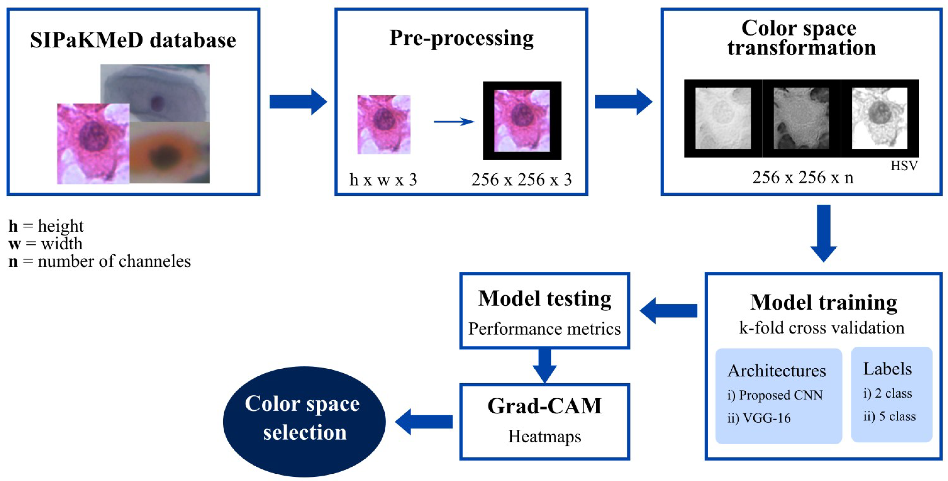
Figure 1 illustrates the work’s block diagram. The proposed research leverages the re-accommodation of pixels after a color space transformation, individual channel selection, and combinations to enhance classification metrics. Yet, it focuses on the cases where abnormal images were sorted as normal, since misclassifying a sick cell image could be potentially more dangerous. The SIPakMeD database was selected for this research because it allows for classification based on cellular appearance and morphological characteristics.

The first stage is image preprocessing, where the images are resized to work in a specific format and size. Every image was resized into $256\times 256$ pixels. Then, six strategies of color space transformation were applied, converting the images from RGB color space to HSV, CMYK, CIELAB, YUV, and grayscale models. RGB channel combinations were implemented, resulting in two-channel matrices corresponding to the red and green (RG), red and blue (RB), and green and blue (GB) channels. Additionally, individual RGB channels were used as input for a classification model.

The training model block corresponds to the proposed CNN or VGG-16 architectures that categorize the images into either two or five classes. To evaluate which color space transformation provided the most relevant information for the classification task, performance metrics such as the F1-score were calculated for each model. Additionally, Gradient-weighted Class Activation Mapping (Grad-CAM) was applied to visualize the regions of interest emphasized by the CNN during prediction.

3.1. SIPakMeD Dataset

The SIPakMeD dataset [24] consists of 4049 images manually cropped from isolated cell images obtained from 966 clusters of cells on Pap smear slides. The images were captured using a CCD camera (Infinity 1, Lumenera) adapted for use with an optical microscope (OLYMPUS BX53F).

Among the collected images, there are five types of cells: dyskeratotic, considered an abnormal cell, with the database containing 813 images of this class; koilocytotic, considered an abnormal cell, with the database containing 825 images of this class; parabasal cells, considered normal cells, with the database containing 787 images of this class; superficial intermediate, considered a normal cell, with the database containing 831 images of this class; metaplastic, considered a benign cell, with the database containing 793 images of this class; however, the presence of these types of cells is associated with precancerous lesions.

Under this context, there is a total of 1618 normal cell images and 2431 abnormal cell images. These will be used to train and test the proposed CNN for classification. It is worth noting that 26 of the 4049 images lacked information regarding the identification of the nucleus and cytoplasm (18 koilocytic, 1 metaplastic, and 7 superficial intermediate), resulting in only 4023 valuable images in the collection.

3.2. Image Preprocessing

The SIPakMeD dataset provides images with isolated cells of different sizes. The minimum and maximum sizes corresponded to dyskeratotic cells, with a size of $40\times 90$ pixels, and superficial-intermediate cells, with a size of $553\times 388$ pixels, respectively, with an average size of $300\times 239$ pixels. The final size selected was $256\times 256$ pixels, taking into account the average size, computational efficiency, and model comparability. A smaller input reduces memory usage, and this size allows for training of well-established DL architectures such as VGG or ResNet, facilitating benchmarking and future work. Resizing was performed using the bilinear interpolation method included in the OpenCV library [29], with different scales depending on the image size. Images larger than the selected size were reduced by a scale factor of less than one. While the images below are of the selected size, they were increased using a scale factor greater than one. 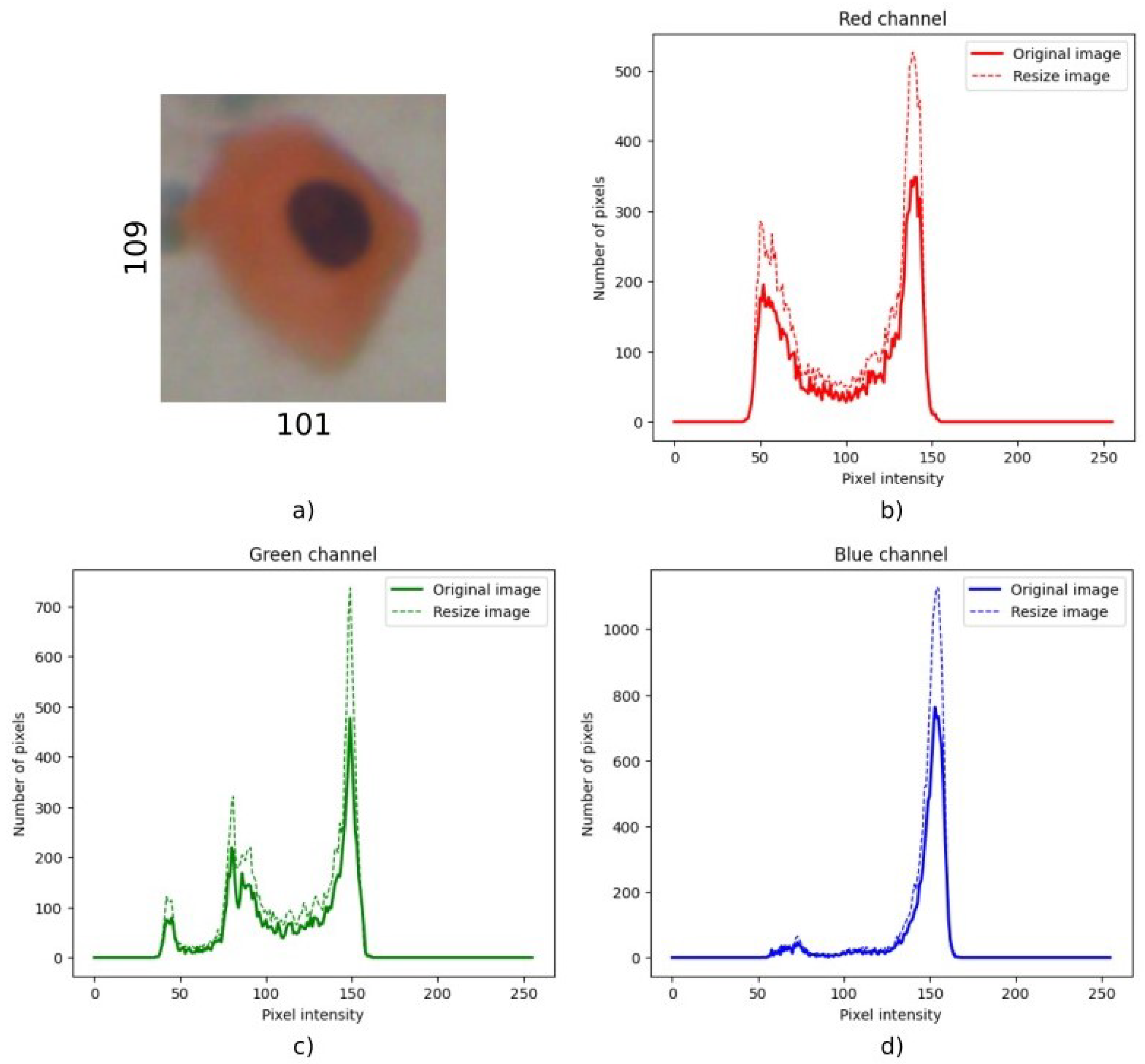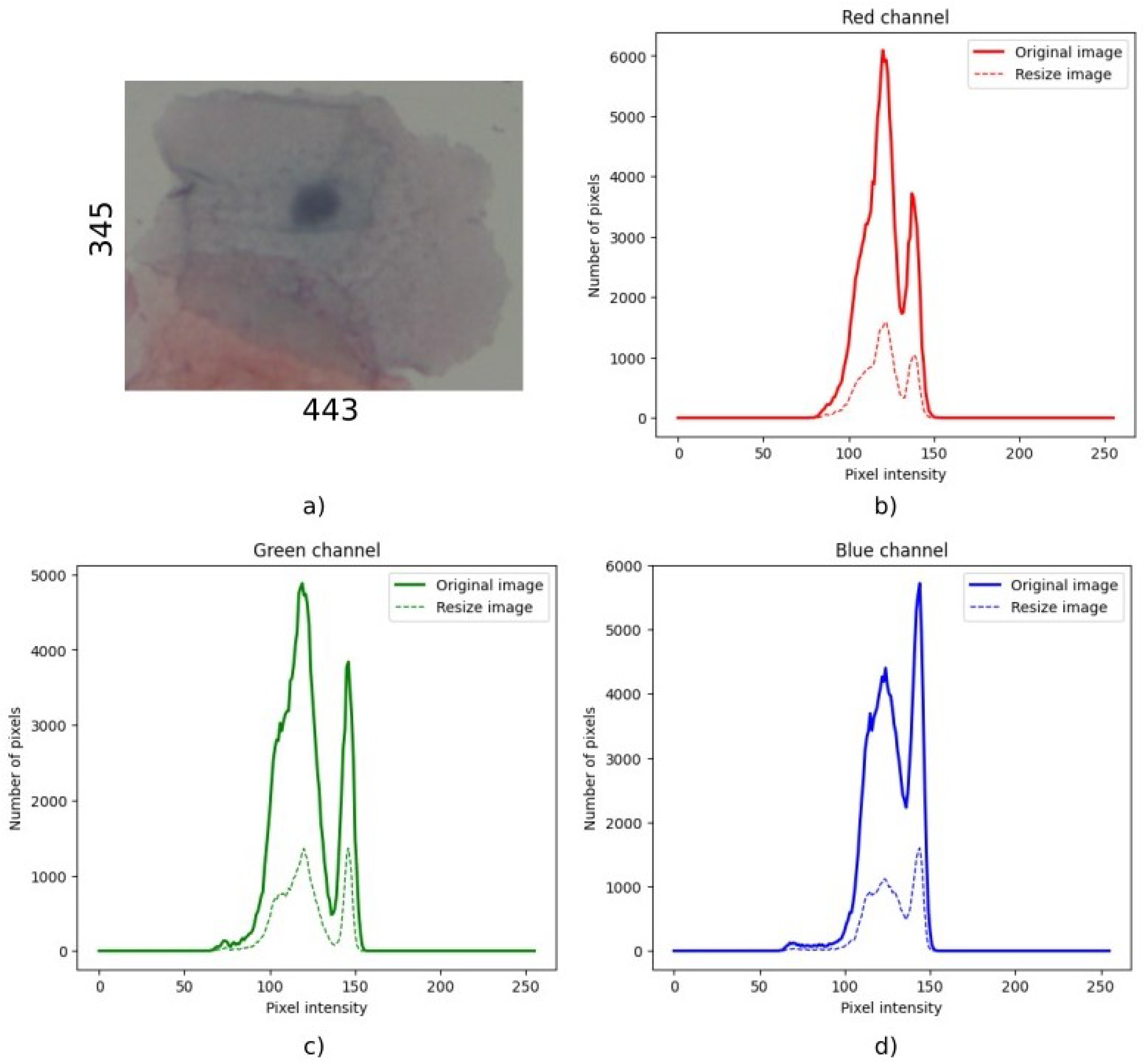To avoid distortion of the nucleus, zero padding was added to fit the images to a $256\times 256\times 3$ matrix when they were close enough to the selected standard size. Therefore, resizing the image to the selected size did not require proportion changes. This should ensure that the rescaling process did not alter the distribution of pixel intensities, a finding later confirmed by the preservation of the histogram shape. The main effect was an increase or decrease in the total number of pixels. Figure A1 and Figure A2 in Appendix A show two histogram distributions of an original and resized sample for both cases.

3.3. Data Augmentation

One of the issues in DL models is the requirement for a large dataset to be trained. Medical image tasks can be challenging due to patient privacy concerns, data scarcity, and imbalanced data collection. Under this scenario, data augmentation is often employed to increase data, diversify it, reduce overfitting, and improve the model’s generalization [30]. In this study, data augmentation was applied before training the model through a random flip and a ±10° rotation, both of which were applied with a 50% probability. After this process, a normalization operation was carried out on every cell image by scaling pixel values from the original [0–255] range to [0–1] using the ToTensor function of PyTorch version 2.8, which also converts the image format from [H, W, C] to [C, H, W], where H, W, are the height and width of the images, respectively.

3.4. Color Space Transformations

The colors humans perceive in an object are the light reflected from the object. This light corresponds to the visible portion of the electromagnetic spectrum, which spans wavelengths from approximately 400 nm (blue) to 700 nm (red). For example, a yellow object reflects light with wavelengths in the range of 570 to 580 nm. Human color vision exists because of the 6 to 7 million cone cells in the retina, which are sensitive to three wavelength ranges corresponding to the colors red, green, and blue. As a result, people see color as the combination of these primary colors.

To distinguish among different colors, there are three principal properties: brightness, hue, and saturation. The brightness refers to the intensity of the color; hue is associated with the position in the visible spectrum; and the saturation refers to the amount of white light mixed with a hue. Color spaces were created to standardize and represent color components. Color space models are mathematical models that are able to represent colors as points in a coordinate space. They are widely used in multiple applications across fields such as computer vision, image processing, and computer graphics, as their properties can facilitate image processing tasks [31,32].

3.4.1. HSV Model

The HSV model is a cylindrical color model that represents colors based on hue (H, type of color), saturation (S, intensity), and value (V, brightness). The hue component goes from 0° to 360° to represent all colors. Saturation (S) represents the colorfulness. If a hue is further from the cylinder center, the color will be saturated, while if it is near the center, it will appear as shades of gray. The value (V) defines the brightness of the hue, causing the colors to change from black to white. The HSV model is intuitive for color selection in graphics and image editing because it provides a practical human interpretation compared to the RGB and CMYK models. However, its transformation is less intuitive than the CMYK model. Additionally, since information about the visible spectrum is contained in a single channel, the remaining channels provide unique details not available in other color spaces.

The procedure for converting an RGB image to HSV color space begins by normalizing the image range from [0, 255] to [0, 1]. Then, the maximum ($C_{max}$) and minimum ($C_{min}$) values from each RGB channel must be found, and their difference must be calculated ($\Delta =C_{max}-C_{min}$). The conversion formulas for H, S, and V channels are given in Equation (1), Equation (2), and Equation (3), respectively [33].

$$H=\left\{\begin{array}{ccc}0,\hfill & \hfill & C_{\max }=0,\hfill \\ 60\times {\displaystyle \frac{G-B}{\Delta }},\hfill & \hfill & C_{\max }=R,\hfill \\ 60\times {\displaystyle \frac{B-R}{\Delta }}+120,\hfill & \hfill & C_{\max }=G,\hfill \\ 60\times {\displaystyle \frac{R-G}{\Delta }}+240,\hfill & \hfill & C_{\max }=B.\hfill \end{array}\right.$$

(1)

$$S=\left\{\begin{array}{ccc}{\displaystyle \frac{\Delta }{C_{max}}},\hfill & \hfill & C_{\max }=0,\hfill \\ 0,\hfill & \hfill & C_{\max }=0.\hfill \end{array}\right.$$

(2)

$$V=C_{max}.$$

(3)

3.4.2. CMYK Model

The CMYK model is a subtractive color model in which the principal colors are the complementary pigments: cyan, magenta, yellow, and black (key). It works by absorbing light, with black (K) added to improve depth and contrast. The transformation from RGB to CMYK involves subtracting each component (R, G, and B) from white to create the C, M, and Y channels (that is, C = (1-R), M = (1-G), Y = (1-B)); the K channel is formed with minimum values of each C, M, and Y channel. Equation (4) shows the mathematical transformation for them. It is worth mentioning that the image must be normalized to the [0–1] range.

$$C={\displaystyle \frac{(C-K)}{(1-k)}},M={\displaystyle \frac{(M-K)}{(1-k)}},Y={\displaystyle \frac{(Y-K)}{(1-k)}}$$

(4)

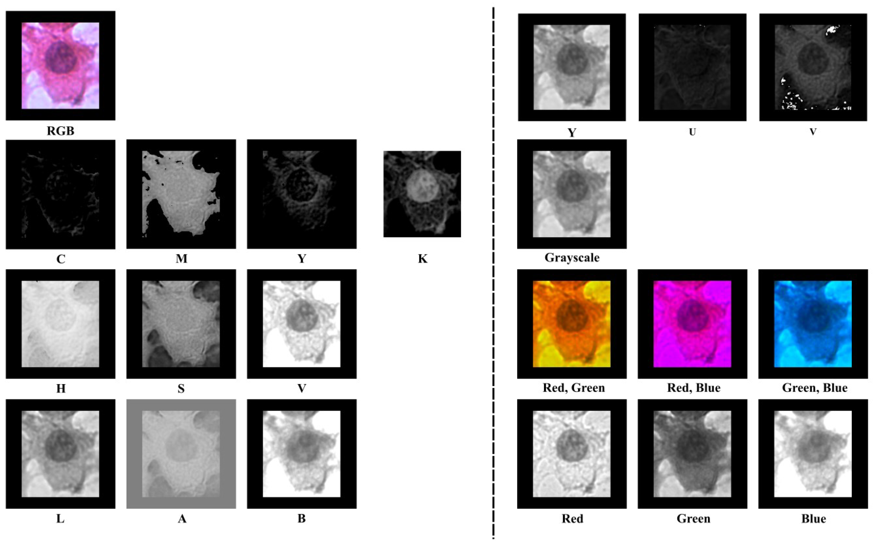
Figure 2 displays the decomposed channels of each color space, showing how each transformation encodes the chromatic and luminance information. This visualization is adapted to the screen it will be shown on or the paper it will be printed on, since the color space and output device cannot be separated.

3.5. Classification Model

CNNs have been the most used DL technique in medical image analysis. They can capture spatial hierarchies and extract features from the input through convolutional and pooling layers. However, a CNN architecture consists of more building blocks that lend training stability and generalization, such as nonlinear activation function layers, dropout, batch normalization, and fully connected layers. The combination of these operations enables the extraction and classification of complex features [34,35,36].

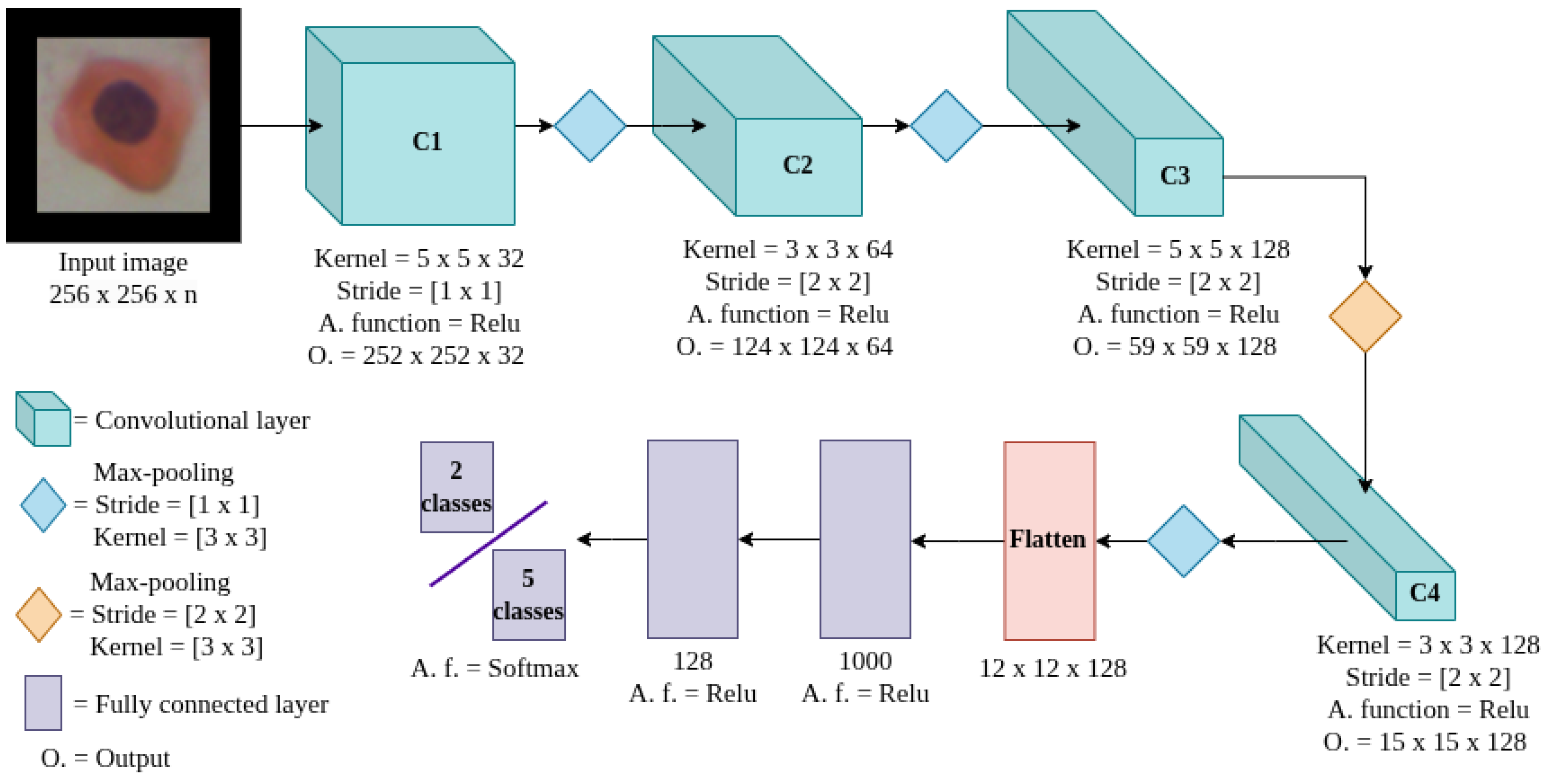
In this work, we designed a CNN model to analyze the dataset for both binary and five-class classification tasks. The LeNet model [37] served as the base for our proposed CNN; the parameters were determined through an exhaustive grid search, using the RGB space model as input. The network architecture consisted of four convolutional layers, followed by two fully connected layers and an output layer. The first convolutional layer used a $5\times 5$ kernel with a stride of one. The subsequent convolutional layers employed a stride of two; the second layer used a $3\times 3$ kernel, the third a $5\times 5$ kernel, and the final convolutional layer also used a $3\times 3$ kernel. Batch normalization was applied after each convolutional layer, and all layers employed the ReLU activation function. Max-pooling operations with a $3\times 3$ window and a stride of one were used after each convolutional layer, except for the third max-pooling layer, which used a stride of two. The interleaved structure of large and small kernels was intended to capture both coarse features through larger receptive fields and fine-grained details through smaller ones, thereby enhancing feature representation across spatial scales. Mingxing Tan and colleagues studied the impact of using different kernel sizes, such as $3\times 3$, $5\times 5$, and $7\times 7$, and reported the improvement in metrics for using a different kernel in a single convolutional layer [38]. The use of big kernels had also been demonstrated as a powerful paradigm in contrast to the use of small kernels [39].

The previous layers perform the feature extraction from the input images. After this process, the resulting feature maps were concatenated to begin the classification technique. Two fully connected layers were used to sort the data, each with a ReLU activation function. The output layer consisted of either two or five neurons, depending on the strategy (binary or five-class classification) and the use of the Softmax activation function. Figure 3 shows the whole model, the kernel size, the number of neurons in each fully connected layer, and the feature map size output of each convolutional layer.

VGG-16

To compare and validate our proposal, we utilize the VGG-16 architecture [40], which consists of a deep CNN with small convolution filters in all layers. The model achieved a test data accuracy of 92.77% using ImageNet. They highlighted the importance of a deep model in visual representations.

4. Experiments and Results

All the experiments for our CNN architecture were run on a computer equipped with an Intel Core i7-13th generation processor and an NVIDIA RTX 4070 GPU with 8GB of RAM. The experiments using the VGG-16 model were implemented on a computer with an Intel Core i7-8th generation processor and two GPUs, 1080Ti, with 12 GB of RAM each. The algorithms were coded in Python 3.11.5 using the Pytorch framework.

Table 1. Hyperparameters for both architectures.

Hyperparameters
Learning Rate	0.001
Batch size	32
Optimizer	ADAM
Loss function	Cross-entropy
Epochs	200

summarizes the hyperparameters for both architectures.

A 5-fold cross-validation scheme was applied in all experiments. The data augmentation and color space transformations were applied online to save memory and automate the experiments.

4.1. Binary Classification Results

For the binary classification task, both the abnormal and normal classes consisted of 1611 images each. These datasets were used to evaluate 12 different color space transformations and RGB channel combinations, tested with both the proposed CNN and the VGG-16 architecture. For each color model and architecture, ten confusion matrices were generated. All results are available in our repository.

The best average F1-scores per fold obtained with the proposed CNN are as follows: fold 0 for RGB (0.9736), fold 3 for CMYK (0.9891), fold 0 for HSV (0.9891), fold 1 for CIELAB (0.9814), fold 3 for YUV (0.9674), fold 1 for grayscale (0.9549), fold 2 for RG (0.9627), fold 0 for RB (0.9720), fold 1 for GB (0.9798), fold 4 for the R channel (0.9519), fold 3 for the G channel (0.9564), and fold 4 for the B channel (0.9487).

For the VGG-16 model, the best average F1-scores per fold are as follows: fold 0 for RGB (0.9752), fold 0 for CMYK (0.9519), fold 0 for HSV (0.9674), fold 0 for CIELAB (0.9658), fold 1 for YUV (0.9550), fold 2 for grayscale (0.9518), fold 0 for RG (0.9566), fold 2 for RB (0.9534), fold 2 for GB (0.9658), fold 1 for the R channel (0.9083), fold 0 for the G channel (0.9347), and fold 2 for the B channel (0.9392).

4.2. Classification of the Five Classes

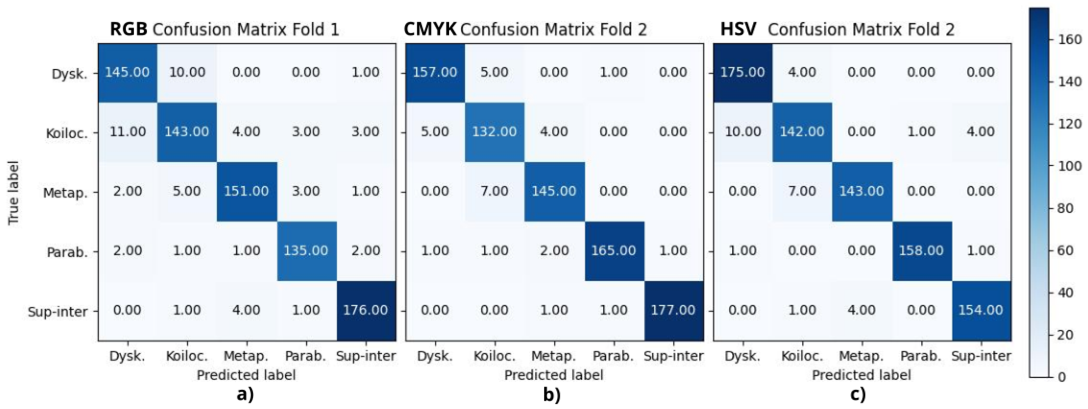
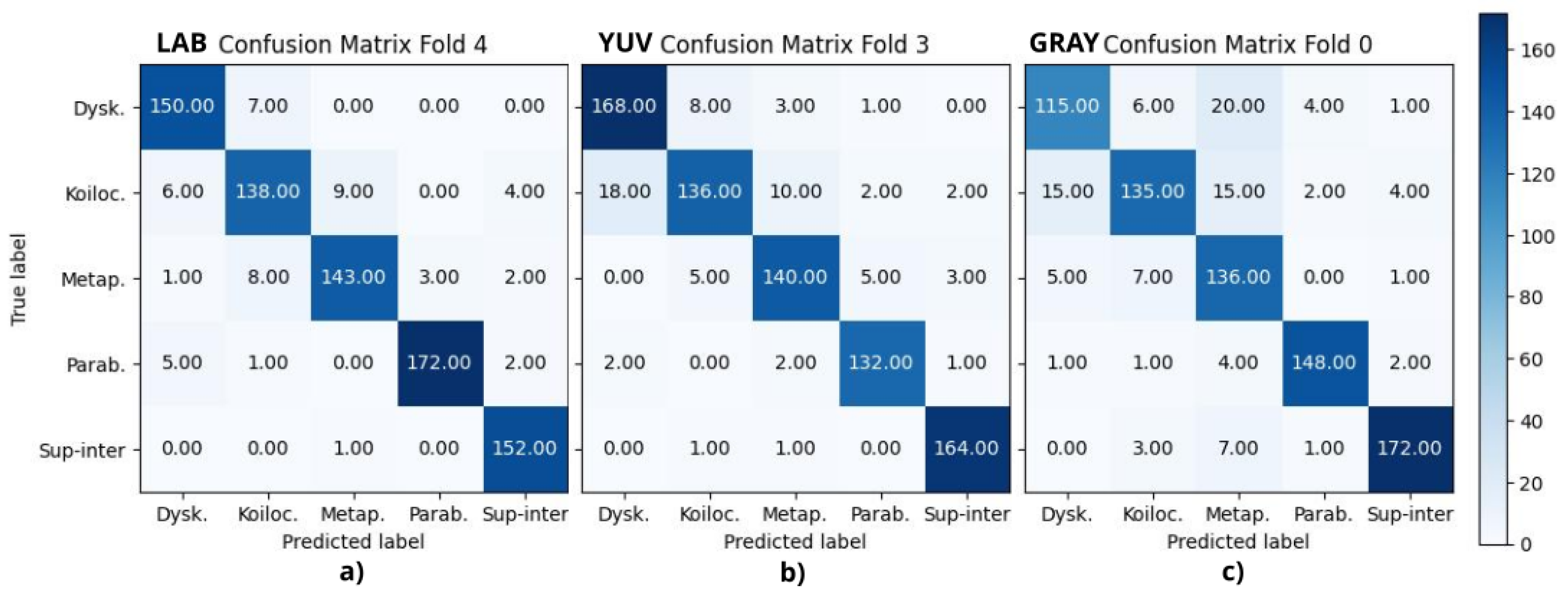
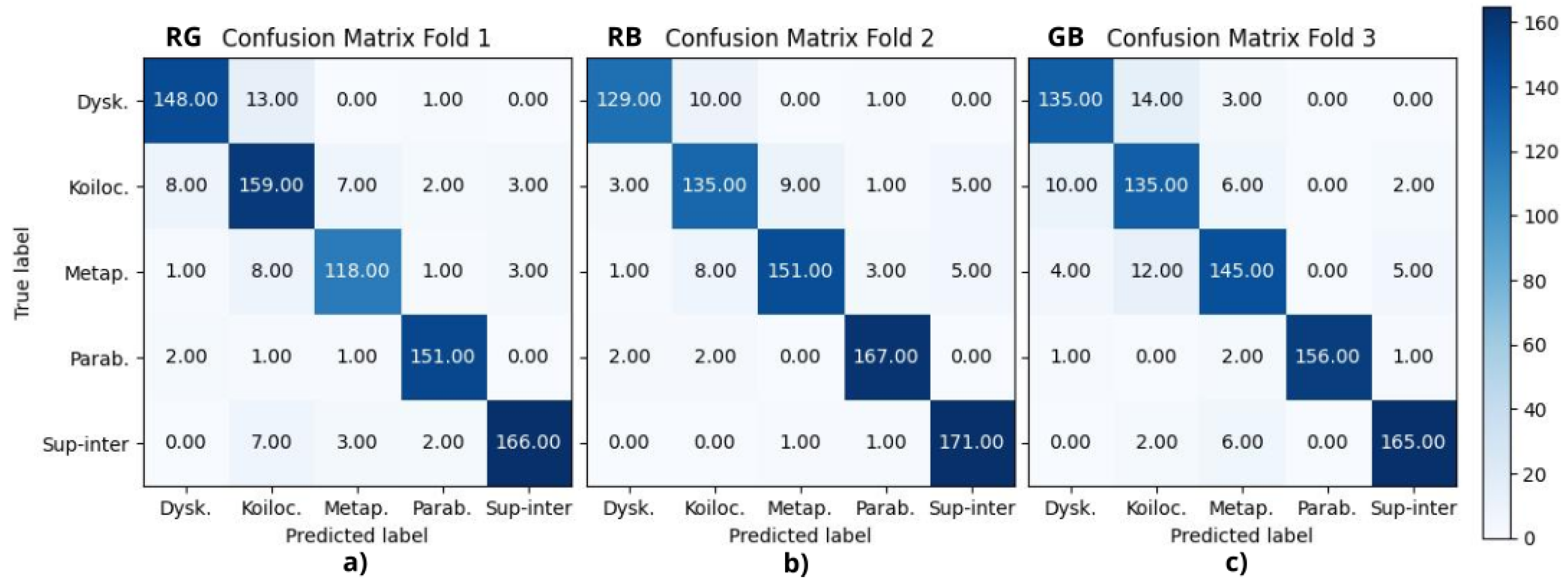
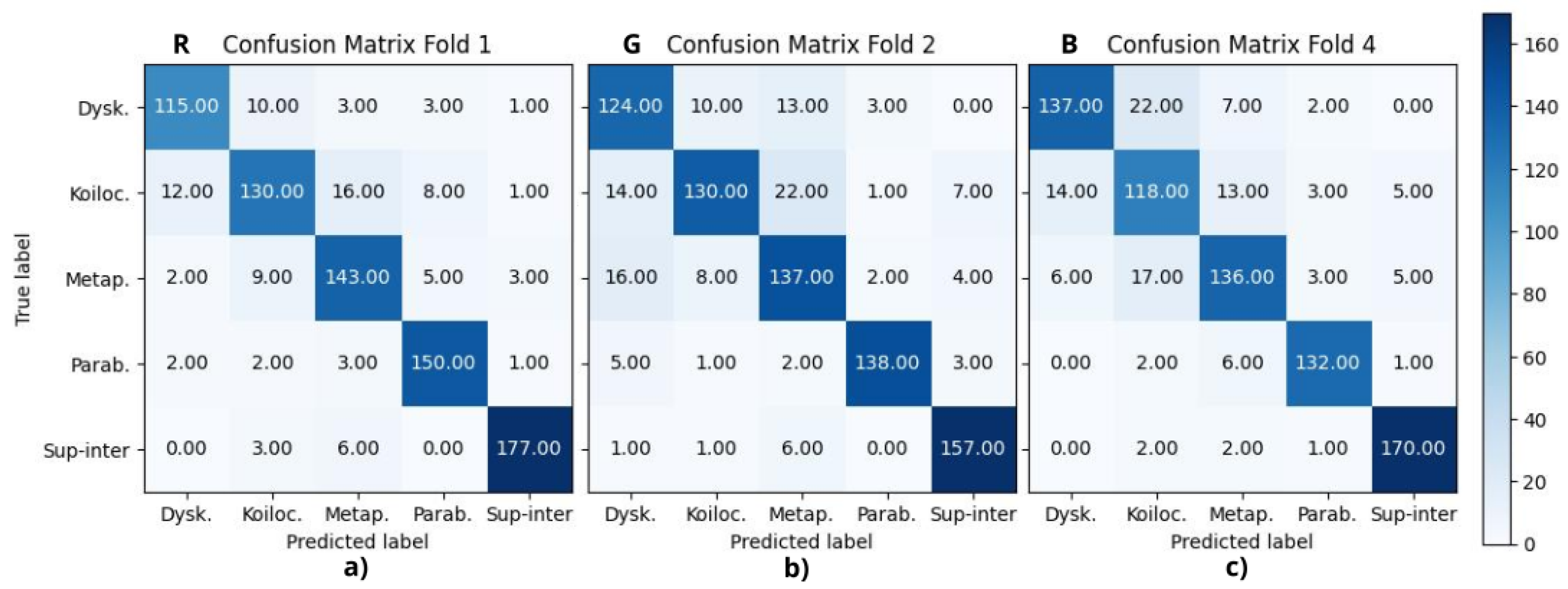
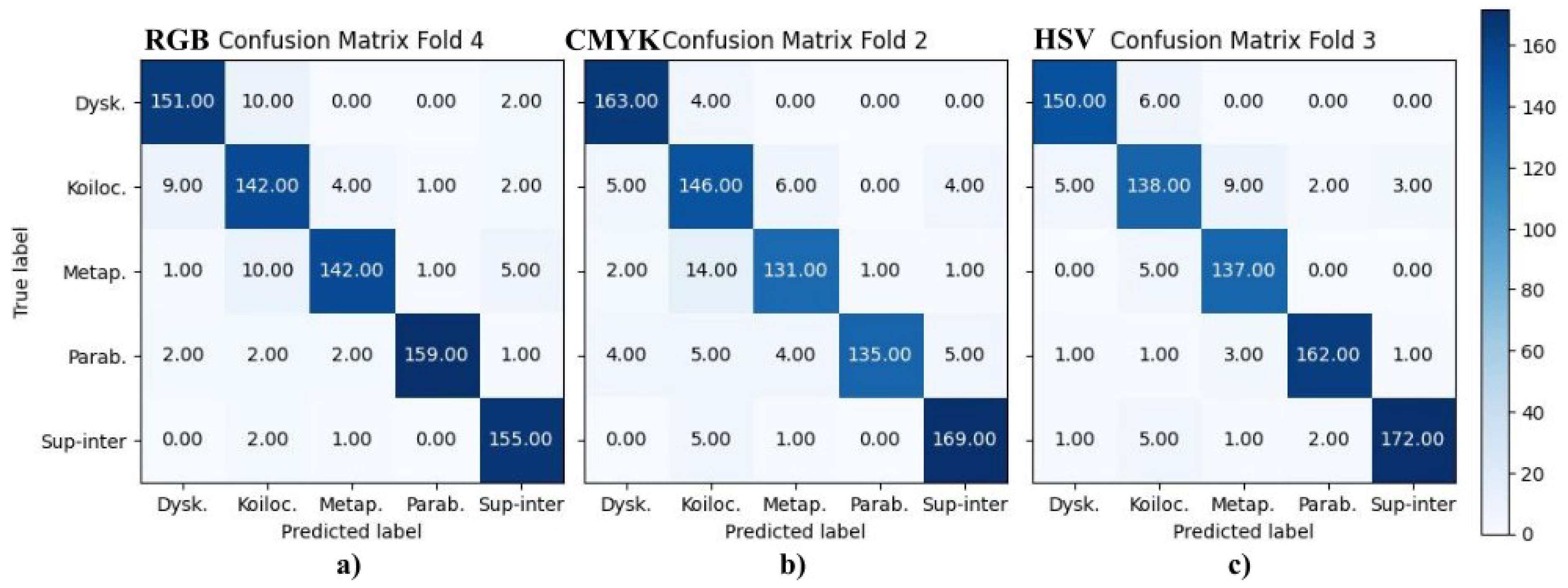
The results of the classification of the five types of cells are shown in Figure 4, where the best fold from RGB, CMYK, and HSV experiments corresponds to (a) fold 1, (b) fold 2, and (c) fold 2, respectively.

Figure 5 displays the best fold from CIELAB, YUV, and grayscale experiments, where (a) corresponds to fold 4, (b) to fold 3, and (c) to fold 0, respectively.

Figure 6 presents the best fold from the combinations of RGB color space channels from RG, RB, and GB experiments, where (a) corresponds to fold 1, (b) to fold 2, and (c) to fold 3, respectively.

Finally, Figure 7 shows the best fold from each RGB channel, R, G, and B experiments, where (a) corresponds to fold 1, (b) to fold 2, and (c) to fold 4, respectively.

The results of the VGG-16 models are shown in Figure 8, which presents the best results from the RGB, CMYK, and HSV color transformations, where (a) corresponds to fold 4, (b) to fold 2 and (c) to fold 3, respectively.

Grad-CAM

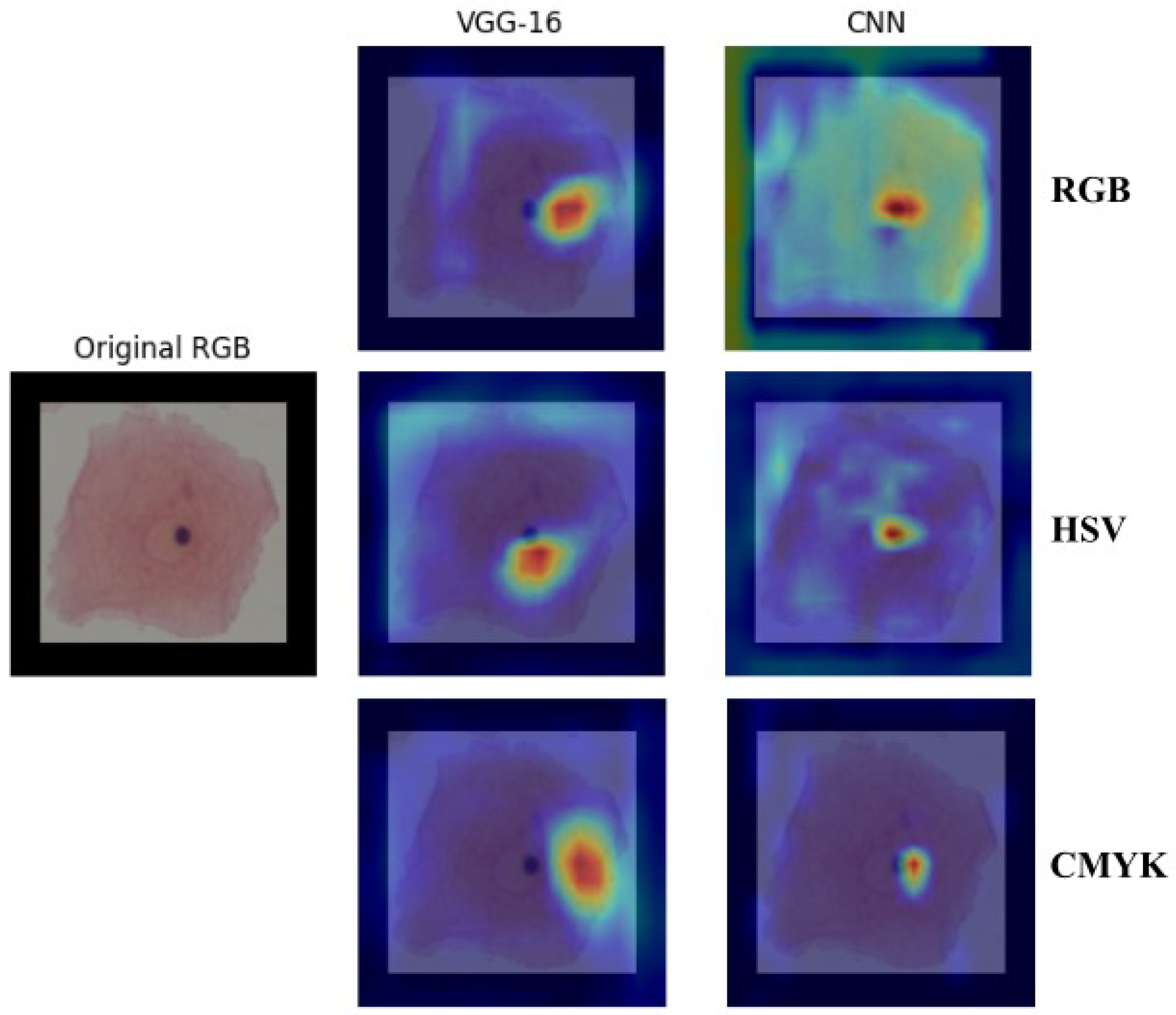
Additionally, the Grad-CAM algorithm [41] was used to select the color space based on the characteristics that each model chose to inform its decision. In Figure 9, an example of the relationship between the RGB, HSV, and CMYK color spaces for both architectures can be observed. Warmer colors (red/yellow) indicate areas with higher contributions to the decision, while cooler colors (blue) represent less relevant regions.

5. Discussion

To evaluate our methodology, three metrics were calculated: precision, recall, and F1-score.

Table 2. Metrics of multiclass problem.

		Own CNN			VGG-16
Color Space	Class	Precision	Recall	F1-Score	Precision	Recall	F1-Score
RGB	A	0.9063	0.9295	0.9177	0.9264	0.9264	0.9264
	B	0.8938	0.8720	0.8827	0.8554	0.8987	0.8765
	C	0.9438	0.9321	0.9379	0.9530	0.8931	0.9221
	D	0.9507	0.9574	0.9541	0.9876	0.9578	0.9725
	E	0.9617	0.9670	0.9644	0.9394	0.9810	0.9598
CMYK	A	0.9632	0.9632	0.9632	0.9368	0.9760	0.9560
	B	0.9103	0.9362	0.9231	0.8391	0.9068	0.8716
	C	0.9539	0.9539	0.9539	0.9225	0.8792	0.9003
	D	0.9880	0.9706	0.9792	0.9926	0.8824	0.9343
	E	0.9944	0.9888	0.9916	0.9441	0.9657	0.9548
HSV	A	0.9409	0.9777	0.9589	0.9554	0.9615	0.9585
	B	0.9221	0.9045	0.9132	0.8903	0.8790	0.8846
	C	0.9728	0.9533	0.9630	0.9133	0.9648	0.9384
	D	0.9937	0.9875	0.9906	0.9759	0.9643	0.9701
	E	0.9686	0.9686	0.9686	0.9773	0.9503	0.9636
CIELAB	A	0.9259	0.9554	0.9404	0.9398	0.9017	0.9204
	B	0.8961	0.8790	0.8875	0.7816	0.8718	0.8242
	C	0.9346	0.9108	0.9226	0.8726	0.8839	0.8782
	D	0.9829	0.9556	0.9690	0.9745	0.9444	0.9592
	E	0.9500	0.9935	0.9712	0.9669	0.9182	0.9419
YUV	A	0.8936	0.9333	0.9130	0.8696	0.9143	0.8914
	B	0.9067	0.8095	0.8553	0.8193	0.8047	0.8119
	C	0.8974	0.9150	0.9061	0.8037	0.9097	0.8534
	D	0.9429	0.9635	0.9531	0.9128	0.8947	0.9037
	E	0.9647	0.9880	0.9762	0.9667	0.8430	0.9006
Grayscale	A	0.8456	0.7877	0.8156	0.8081	0.8035	0.8058
	B	0.8882	0.7895	0.8359	0.6918	0.8209	0.7509
	C	0.7473	0.9128	0.8218	0.7956	0.7517	0.7730
	D	0.9548	0.9487	0.9518	0.9819	0.8717	0.9235
	E	0.9556	0.9399	0.9477	0.9294	0.9576	0.9433
RG	A	0.9308	0.9136	0.9221	0.9086	0.9636	0.9353
	B	0.8457	0.8883	0.8665	0.8476	0.8274	0.8373
	C	0.9147	0.9008	0.9077	0.8070	0.8846	0.8440
	D	0.9618	0.9742	0.9679	0.9714	0.9067	0.9379
	E	0.9651	0.9326	0.9486	0.9675	0.9030	0.9342
RB	A	0.9556	0.9214	0.9382	0.8994	0.9325	0.9157
	B	0.8710	0.8824	0.8766	0.7738	0.8280	0.8000
	C	0.9379	0.8988	0.9179	0.8266	0.8563	0.8412
	D	0.9653	0.9766	0.9709	0.9554	0.8982	0.9259
	E	0.9448	0.9884	0.9661	0.9416	0.8600	0.8990
GB	A	0.9000	0.8882	0.8940	0.8957	0.8488	0.8716
	B	0.8282	0.8824	0.8544	0.7443	0.8037	0.7729
	C	0.8951	0.8735	0.8841	0.7750	0.8322	0.8026
	D	1.0000	0.9750	0.9873	0.9304	0.9188	0.9245
	E	0.9538	0.9538	0.9538	0.9730	0.8944	0.9320
R	A	0.8779	0.8712	0.8745	0.8252	0.7613	0.7919
	B	0.8442	0.7784	0.8100	0.7500	0.6977	0.7229
	C	0.8363	0.8827	0.8589	0.7929	0.8645	0.8272
	D	0.9036	0.9494	0.9259	0.8235	0.9032	0.8615
	E	0.9672	0.9516	0.9593	0.9509	0.9226	0.9366
G	A	0.7750	0.8267	0.8000	0.8242	0.8671	0.8451
	B	0.8667	0.7471	0.8025	0.7484	0.7436	0.7460
	C	0.7611	0.8204	0.7896	0.7535	0.6688	0.7086
	D	0.9583	0.9262	0.9420	0.8987	0.9467	0.9221
	E	0.9181	0.9515	0.9345	0.9226	0.9337	0.9281
B	A	0.8726	0.8155	0.8431	0.7892	0.8588	0.8225
	B	0.7329	0.7712	0.7516	0.7368	0.6292	0.6788
	C	0.8293	0.8144	0.8218	0.7115	0.7070	0.7093
	D	0.9362	0.9362	0.9362	0.8649	0.9143	0.8889
	E	0.9392	0.9714	0.9551	0.9264	0.9497	0.9379

reports the final metrics using the above confusion matrices, where A, B, C, D, and E correspond to dyskeratotic, koilocytotic, metaplastic, parabasal, and superficial–intermediate samples, respectively. CMYK and HSV had all their F1-scores above 90%, being consistent with the binary case. RGB, CIELAB, YUV, and RB combinations had four scores above 90%; in all of them, koilocytotic samples had the lowest value. However, when analyzing the values independently per class, there was no clear ranking or consistent pattern that suggested one color space outperformed the others across all classes.

The current analysis suggests that the metrics may not be a definitive criterion for defining the best color model. It is necessary to consider the misclassifications observed in the confusion matrices. The focus was oriented to False Positive (FP) results, that is, abnormal cells misclassified as normal samples, given that this confusion is more critical than a False Negative result. In this case, the upper-right quadrant of the confusion matrix is particularly relevant, where either dyskeratotic, koilocytic, or metaplastic cells are wrongly classified as parabasal or superficial–intermediate. To quantify this, two parameters were considered: (1) the total number of misclassifications in this quadrant and (2) the number of zero-valued cells (categories with no errors). Using the proposed CNN, HSV, and CMYK exhibited the best performance, followed by GB. For the VGG-16 model, HSV and CMYK also had the best results along with CIELAB. Both cases reported alternative color spaces that performed better than the original RGB of the images. Additionally, in both cases, HSV and CMYK were among the top three in performance.

For the binary case, a similar analysis was conducted. Through the proposed CNN model, HSV, CMYK, and GB combinations produced the lowest number of FP. In comparison, the VGG-16 architecture had the HSV, RG, and RB combinations with the lowest number of FP. This reinforces the idea that switching to alternative color spaces can enhance classification. Additionally, in both the binary and multiclass cases, HSV performed better than the RGB color space. However, since the ranking was not consistent in the one-on-one order comparison, it is suggested to consider not only the HSV color space but also the CMYK as viable options to differentiate between normal and abnormal cells.

Aside from differentiating between normal and abnormal cells, it is also essential to be able to identify specific abnormal cell types, as the presence of certain cells may indicate a particular condition. Focusing on the upper-left quadrant, the classification of these cell types in the HSV, CMYK, and CIELAB color spaces resulted in fewer misclassification cases for both models.

When comparing our results with those reported in [25] using the HSV color space, the F1-scores are similar, with a maximum difference of 3%. This suggests that the use of alternative color spaces is a practical approach for classifying cervical cytology. However, when considering the RGB color space, our metrics are comparatively lower. It could be attributed to the image resolution: using smaller image sizes might reduce the number of faded or noisy pixels, potentially improving classification metrics. Even so, the maximum difference is only 5%, which is not substantial enough to invalidate our approach. These findings support the relevance and robustness of our methodology for future research.

The Grad-CAM analysis highlights the specific area that the model focuses on for class differentiation; in Figure 9, the three color spaces show a main focus on the nucleus of the cell. However, in the proposed model, the RGB model also has a relatively high gradient in the cytoplasm. This dispersion of attention may be another factor contributing to its lower performance. Additionally, when comparing our model to the VGG-16 architecture, the attention focus is slightly displaced to the left in the VGG-16, emerging from the nucleus, whereas the proposed model focuses on the nucleus’s center.

Lastly, the computational time and cost of transforming color spaces were also taken into consideration. Among all, the RGB to CIELAB conversion required significantly more processing time than the rest. Given this, and its lower performance in comparison to false positives, CIELAB may not be suitable for practical implementation, despite its theoretical potential.

6. Conclusions

The proposed model’s obtained results are comparable to those reviewed in the state of the art. Having a simpler model with positive results may lead to a future portable application. As the results point out and the discussion synthesizes, changing the information contained in an image to a different color space can improve the classification results using DL models. In both cases, the binary and multiclass classification, the HSV color space obtained the highest performance, yet CMYK and the GB channel combination had equivalent results when differentiating normal and abnormal cells. In this context, it is advisable not only to work with the RGB color space; using alternative representations, such as HSV or CMYK, can emphasize features in the images that improve classification performance and provide more robust evaluation metrics. Color spaces such as CIELAB, YUV, and Grayscale also had notable performance compared to the original RGB; however, these did not match the performance of the ones mentioned before. The analysis of the independent channels of the RGB color space and the two-channel combinations of such showed that each channel from a color space may provide more or less relevant information for the classification task. Furthermore, the information provided to the DL model does not need to encompass the entire space, as is the case in this study, where only portions of it are considered.

A future study may involve combining channels from different spaces to maximize the valuable information obtained, both for differentiating between normal and abnormal cells and for specifically identifying abnormal cells. Additionally, the current analysis and biological background indicate that the nucleus is the primary characteristic that differentiates a normal cell from an abnormal one. Exploring the bases for implementing binary masks for classification may be beneficial.