Machine Learning Recognition and Phase Velocity Estimation of Atmospheric Gravity Waves from OI 557.7 nm All-Sky Airglow Images

Abstract

Atmospheric gravity waves (AGWs) are treated as density structure perturbations of the atmosphere and play an important role in atmospheric dynamics. Utilizing All-Sky Airglow Imagers (ASAIs) with OI-Filter 557.7 nm, AGW phase velocity and propagation direction were extracted using classified images by visual inspection, where airglow images were collected from the OMTI network at Shigaraki (34.85 E, 134.11 N) from October 1998 to October 2002. Nonetheless, a large dataset of airglow images are processed and classified for studying AGW seasonal variation in the middle atmosphere. In this article, a machine learning-based approach for image recognition of AGWs from ASAIs is suggested. Consequently, three convolutional neural networks (CNNs), namely AlexNet, GoogLeNet, and ResNet-50, are considered. Out of 13,201 deviated images, 1192 very weak/unclear AGW signatures were eliminated during the quality control process. All networks were trained and tested by 12,007 classified images which approximately cover the maximum solar cycle during the time-period mentioned above. In the testing phase, AlexNet achieved the highest accuracy of 98.41%. Consequently, estimation of AGW zonal and meridional phase velocities in the mesosphere region by a cascade forward neural network (CFNN) is presented. The CFNN was trained and tested based on AGW and neutral wind data. AGW data were extracted from the classified AGW images by event and spectral methods, where wind data were extracted from the Horizontal Wind Model (HWM) as well as the middle and upper atmosphere radar in Shigaraki. As a result, the estimated phase velocities were determined with correlation coefficient (R) above 0.89 in all training and testing phases. Finally, a comparison with the existing studies confirms the accuracy of our proposed approaches in addition to AGW velocity forecasting.

1. Introduction

The atmospheric gravity wave (AGW) is regarded as one of the most important fluctuations in atmospheric density. Since the studies conducted by Hines [1], rigorous research has taken place and AGWs are treated as the primary mechanism in the middle atmosphere responsible for transferring energy from the ground surface to various altitudes.

For several decades, AGW observations have been made by measuring techniques such as radar and All-Sky Airglow Imagers (ASAIs) or Optical Airglow Imagers (OAIs). Regardless of their low measuring uncertainties and reasonable accuracies, the horizontal structures of AGWs were clearly detected by the ASAIs but very hard to observe by radar.

The advantages of ASAI have not eliminated the importance of radar, especially when measuring the background neutral winds, as the wind–wave interaction could lead to wind-filtering effects [2,3] or wave-transferred momentum into the mesosphere and lower thermosphere region after wave damping or breaking due to prompt changes in background wind or temperature [4,5,6].

In ASAIs, the phase velocities of small-scale atmospheric gravity waves with a horizontal wavelength (5–100) km and a short period (<1 h) were observed [7]. Theoretical and observational research have been published to inspect the characteristics and interaction mechanisms of AGWs [8].

In the last few years, the implementation of machine learning (ML) and deep learning (DL) approaches has excelled with a rising trend. However, ML is considered as a subclass of artificial intelligence (AI) which includes training machines on datasets to recognize patterns and help perform predictions, while DL is considered as a subclass of ML which implements image recognition using a neural network with multiple layers. Consequently, convolutional neural networks (CNNs) have been considered very successful in performing image recognition [9]. On the other hand, a neural network (NN) can perform prediction based on specific databases; one such example is a cascade forward neural network (CFNN), where forecasting can be achieved based on identifying, modeling, and extrapolating the patterns found in these databases [10].

Various statistical studies have examined the seasonal variations of horizontal phase speeds and directions of AGWs [11,12,13,14,15,16]. However, predicting AGWs in the mesosphere and lower thermosphere region was a significant challenge. Few studies considered AGW observations in mesosphere regions in comparison to the troposphere and stratosphere layers [17,18,19,20]. As far as we know, one recent study [21] implemented ML approaches to AGW observations near the mesopause region (~90) km. This study involved developing identification processes of localized AGWs and computing their horizontal wavelengths, periods, and directions in ASAIs of OH-Filter (715–930) nm emission at ~87 km. Based on two-step convolutional neural networks (CNNs), they have applied their analysis with a training accuracy of 89.49%. Although, the study did not involve a physics-based approach to estimate the AGW phase velocities, horizontal phase speeds, and directions in the mesosphere region.

In this article, a deep learning-based approach has been introduced for classifying AGW images with georeferenced coordinates. These images were used to extract AGW phase velocity by event and spectral methods, providing an extension of the analysis using OI-557.7 nm emission at ~95 km and broadening the applicability of machine learning at higher altitudes. Nevertheless, AGW and wind data were derived according to a physics-based approach to build a physics-guided database; this database has been used to predict/estimate AGW phase velocity in the mesospheric region using CFNN to ensure physical consistency. To our knowledge, this is the first study that integrates CNN recognition with CFNN regression based on a physics-guided database. The investigation of AGWs is introduced with a comparison to existing studies, these studies correspond to AGW analysis in ASAIs with OI-filter (557.7 nm) located in Shigaraki (34.85 E, 134.11 N), Japan. Beyond the scientific scope, the application of this work can be considered for automating AGW detection and velocity estimation, which can contribute to AGW velocity forecasting and improve prediction.

2. Methodology

2.1. Instrumentation

This work has been conducted through the Optical Mesosphere Thermosphere Imager (OMTI) network at the Institute for Space-Earth Environmental Research, Nagoya University [22]. In the OMTI network, each imager has a fish-eye lens with a field of view 180°, five 3-inch filters on a wheel, and a cooled-CCD camera with 512 × 512 pixels, available online at https://stdb2.isee.nagoya-u.ac.jp/omti/, accessed on 5 April 2025. Since October 1998, synchronized observation of short-period AGWs has been carried out automatically using the imagers at Shigaraki, where the OI (557.7 nm) images are obtained with a time resolution, exposure, and band width of 300 s, 105 s, and 1.78 nm, respectively. Time control was adjusted through the network, and the error was frequently less than 1.0 s. The Shigaraki station is employed to distinguish between different events, such as (a) overcast or rain, (b) clear sky with stars, (c) many clouds and few stars, and (d) few clouds and many stars. Available online at https://stdb2.isee.nagoya-u.ac.jp/omti/obslst.html and accessed on 5 April 2025.

The background wind was extracted from the middle and upper atmosphere (MU) radar located in Shigaraki, Shiga Prefecture, Japan (34.86 N, 136.11 E) [23], available online at http://database.rish.kyoto-u.ac.jp and accessed on 7 June 2025, where the dataset is available online at https://www.rish.kyoto-u.ac.jp/mu/meteor/ which accessed on 7 June 2025. The weighted average data was used for height and time with Gaussian factors of ±1 km and ±60 min, respectively. Since the radar measuring time was taken in Japanese Local Time (LT). This work has been performed based on universal time (UT), and the radar time was converted from Japanese LT to UT.

However, Horizontal Wind Model 14 (HWM-14) was used to fill the radar’s data gaps. HWM is an empirical model that can measure zonal and meridional phase velocity components based on the Fabry–Perot Interferometer (FPI) in equatorial and polar regions, as well as cross-track winds from the Gravity Field and Steady Ocean Circulation Explorer (GOCE) satellite [24]. Finally, when the radar’s neutral wind data were unavailable during the AGW observations, HWM data were used to fill the missing periods from October 1998 to October 2002. The data can be accessed online at https://ccmc.gsfc.nasa.gov/models/HWM14~2014/ on 1 May 2025.

2.2. Data Preparation

2.2.1. Image Extraction

The clear sky and atmospheric gravity waves observational periods were collected in hours per month over Shigaraki. The clear sky hours are extracted according to the OMTI network’s ability to distinguish clear sky periods as mentioned in the Section 2.1, while the atmospheric gravity waves periods were extracted according to the classified AGW images by visual inspection (movie of deviated images in grayscale). The dataset is accessed online at https://ergsc.isee.nagoya-u.ac.jp/data/ergsc/ground/camera/omti/asi/ on 5 April 2025, for the period from October 1998 to October 2002, corresponding to Shigaraki station which labeled “sgk”. The time-period between images is divided into segments, where each segment measures the time difference between two consecutive images only if it is not more than 12 min. Finally, all segments are grouped per month and summated per season in hours.

In Figure 1, clear sky hours and gravity waves observational hours are presented per season. In fall there are 240 and 152.8 h, in spring 284 and 137.5 h, in summer 207 and 103.8 h, and in winter 701 and 369.9 h, respectively. The seasonal criteria for grouping the months per year into fall (September and October), spring (March and April), summer (from May to August), and winter (from November to February) adhered to Nakamura [25]. In total, there are ~1432 h collected for clear sky conditions and ~764 h collected for AGW observations from October 1998 to October 2002.

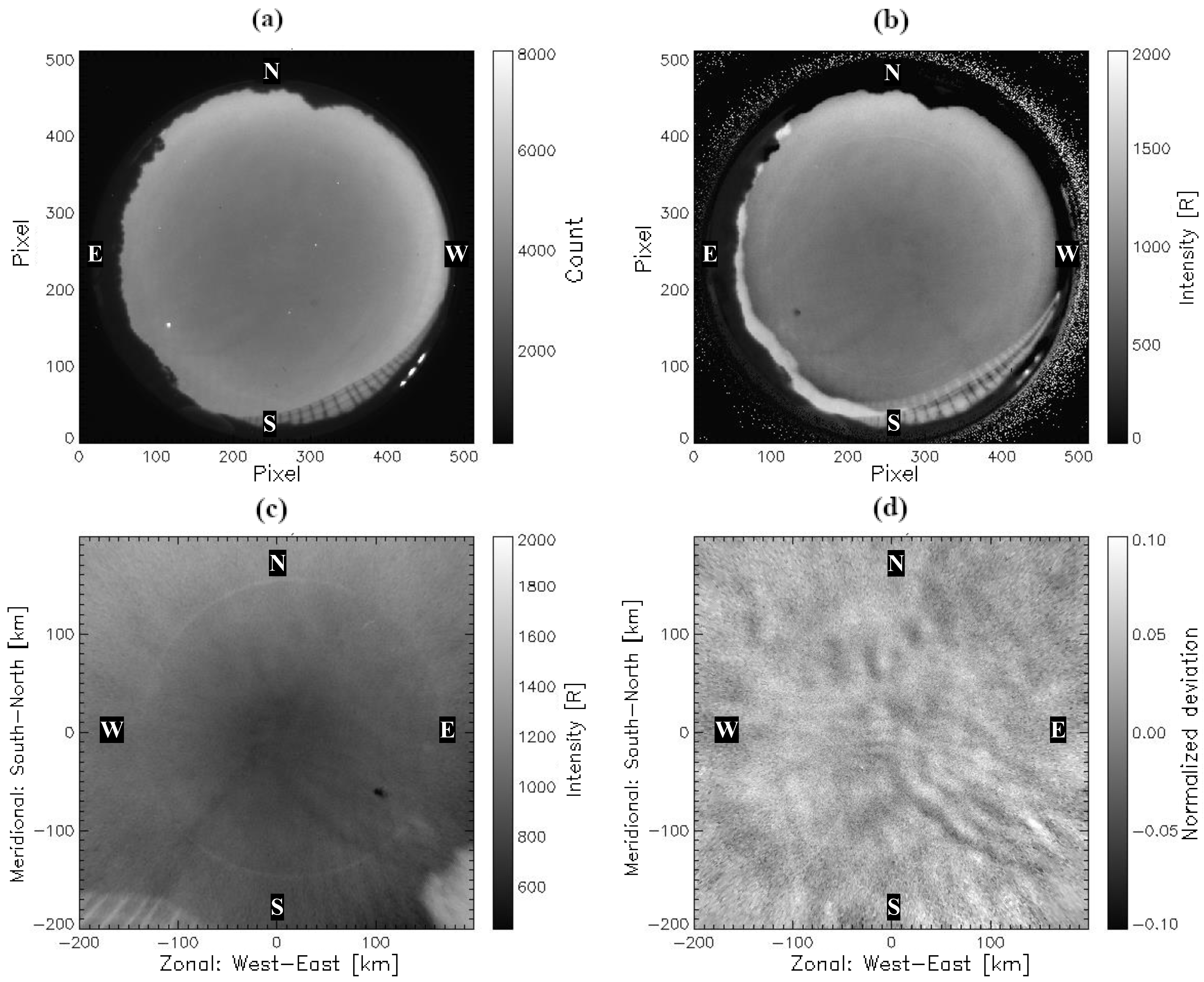
The processes of extracting, mapping, and deviating All-Sky images from the OMTI network are shown in Figure 2; the mentioned processes involve identifying the images’ rotation based on star alignment and recognizing directions by star locations, where all previous steps were as mentioned according to the article [26]. In Figure 2a, the clear sky images are originally extracted with a size of 512 × 512 pixels, giving their geographic coordinates with north at the top position and east at the left position of the image. In Figure 2b, the absolute images are produced by calculating the absolute intensities in Rayleigh units $\left({\displaystyle \frac{{10}^6}{4\pi }}photons {\mathrm{c}\mathrm{m}}^{-2}\mathrm{s}{\mathrm{r}}^{-1}{\mathrm{s}}^{-1}\right)$ which were obtained via the sensitivity data of the imager; this was followed by subtracting the contamination from the background sky emission. Based on the background sky emission at 572.5 nm, as obtained from the calibration data provided on the OMTI servers, the stars were removed using a median filter of width of 21 pixels. In Figure 2c, the absolute images were mapped onto the geographic coordinates with a mapping size of 400 × 400 km², where each pixel corresponds to a grid size of 1 × 1 km².

Finally, in Figure 2d, the normalized deviated images are extracted; this is achieved by subtracting the deviation of each pixel in the mapped image data from a 1 h running average regarding the sequential image data. In the mapped-deviated images, the north–south direction is called the meridional direction with the north direction at the top position of the image, while the east–west direction is called the zonal direction where the east direction is at the right position of the image.

2.2.2. Image Classification

Clear sky images were chosen to be extracted from the OMTI network from October 1998 to October 2002. The overall extracted deviated images are counted as 13,201 images. However, not all clear sky images contain AGW signatures. Accordingly, image classification becomes strongly inevitable. Among 13,201 deviated images, 1194 very weak gravity wave signatures were eliminated to avoid classification bias, while 12,007 deviated images were used for the image classification process as demonstrated in

Table 1. Image classification criteria.

Dataset Stage	Number of Images	Notes
Total deviated images	13,201	Initial dataset from OI-557.7 nm ASAI
Eliminated during quality control process using visual inspection criteria (movie of grayscale images)	1194	Contained very weak/unclear gravity wave patterns, removed to avoid bias during machine learning classification and estimation processes
Final dataset after quality control process	12,007	Used for classification and estimation processes

. The final deviated dataset was chosen based on a quality control process which involved considering visual inspection criteria. This criterion is illustrated by choosing the atmospheric gravity wave signature in a movie of grayscale images.

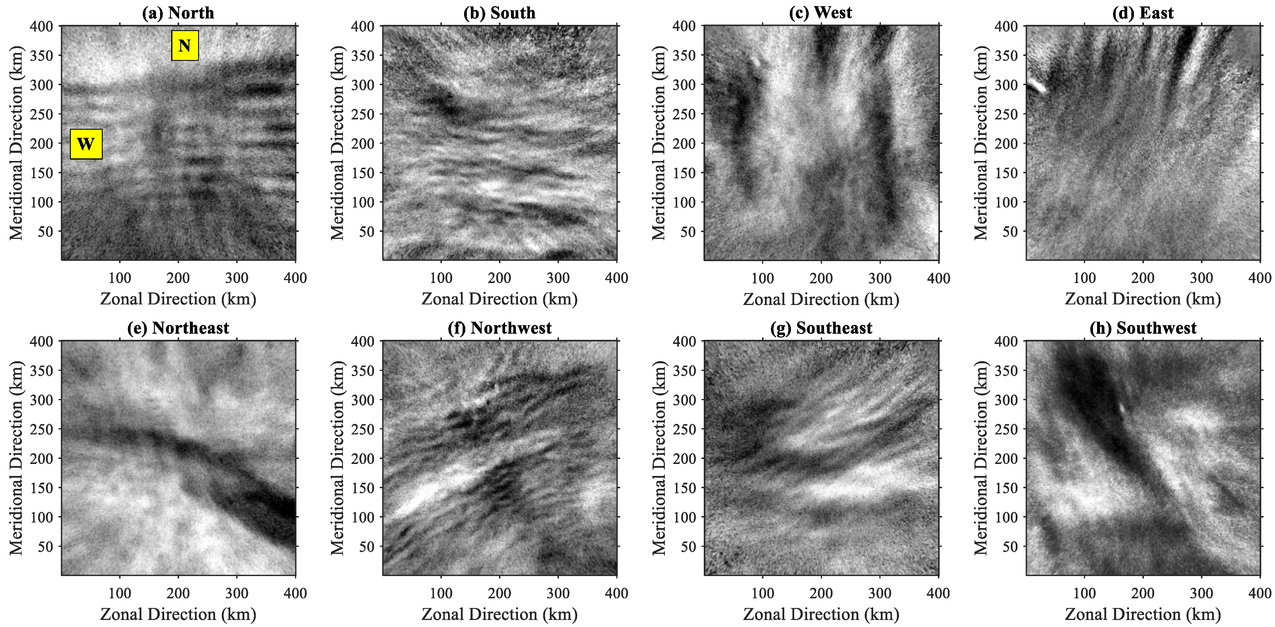
In Figure 3, a sample of AGW images of equal size is presented and regarded as a (GW) class which is elaborated by visual inspection. Each image in the sample set has 400 × 400 pixels which is equivalent to 400 × 400 km². The AGW image sample provided is considered in various directions: Figure 3a, northward; Figure 3b, southward; Figure 3c, westward; Figure 3d, eastward; Figure 3e, northwestward; Figure 3f, northeastward; Figure 3g, southwestward; and Figure 3h, southeastward. On the other hand, non-gravity wave (NGW) images are separated into a different category, which are regarded as a (NGW) class that contains corrupted images or images without AGW signatures.

To automate the classification process mentioned above, convolutional neural networks (CNNs) are suggested. The proposed CNNs are part of the deep learning neural networks (DLNNs) that specify machine learning approaches for image recognition and classification after the training process [27,28].

In Figure 4, the CNN architecture contains the following layers: input, convolution, pooling, fully connected (FC), SoftMax, and output. Notably, convolutional and pooling layers are part of the image feature extraction process. Additionally, FC, SoftMax, and output layers are part of the image classification process.

The first layer is the input layer which takes the 2D deviated image resized to 227 × 227 pixels and 224 × 224 pixels for different CNNs. All input images are enhanced by intensity adjustment to improve the low-contrast image histograms [29] in MATLAB R2023b. Consequently, the convolutional layers start to identify sub-structures and features in the input image, which is performed by convolving with kernels or filters that scan the image. Nonetheless, the rectified linear unit (ReLU) activation function is responsible for reducing the training error rate, while the max-pooling or average pooling layer performs nonlinear down-sampling to reduce the network learning parameters and simplify the output [30].

In classification stage, each neuron in the fully connected (FC) layer has weights from the training process and is connected to the previous layers. Nevertheless, the second activation function (SoftMax) is used for final conclusions by normalizing the outputs and better stating the classification results, based on revealing the classification probability of each neuron in the FC layer [31], according to the highest probability score which the image is classified upon [32].

In this article, three well-known CNNs were subjected to a comparative analysis in the training and testing phases, including AlexNet [30], GoogLeNet [33], and ResNet-50 [34]. All networks were used for image feature extraction. In

Table 2. Network hyperparameters.

Hyperparameters	Best Performance
Network	AlexNet	GoogLeNet	ResNet-50
Epochs	15	15	15
Batch Size	64	64	64
Input size (pixels)	227 × 227	224 × 224	224 × 224
Optimizer	SGDM	SGDM	SGDM
Activation Functions	ReLU, SoftMax	ReLU, SoftMax	ReLU, SoftMax
Learning Rate	1 × 10−4	1 × 10−4	1 × 10−4

, the hyperparameters for the networks are shown. They have been unified and tested to obtain the ideal constraints, which involved comparing the networks based on the prepared image dataset. As every network needs a learning algorithm to be trained, the Stochastic Gradient Descent with Momentum (SGDM) was chosen for all networks because of its high accuracy and minimal loss [35].

To calculate accuracy and precision, the confusion matrix must be introduced, which shows four classification categories: true positive (TP) when AGW images are classified as “gravity waves”, true negative (TN) when non-gravity wave images are classified as “non-gravity waves”, false positive (FP) when non-gravity waves images are classified as “gravity waves”, and false negative (FN) when AGW images are classified as “non-gravity waves” [36]. The “gravity waves” class is labeled “GW”, whereas the “non-gravity waves” class is labeled “NGW”.

Accordingly, the accuracy Equation (1) and precision Equation (2) can be calculated [37], where accuracy means the network’s overall performance, and the result is given by dividing the correct classification over the total classified images of gravity waves and non-gravity waves.

$$\begin{array}{c}Accuracy={\displaystyle \frac{True Positive+True Negative}{Total number of predictions}}\times 100\%\end{array}$$

(1)

In contrast, precision indicates how reliably the network classifies gravity wave images, reflecting the proportion of correctly identified images among those it labeled as TP, which is calculated by dividing the correct classified gravity waves (TP) over the total number of correctly and wrongly classified gravity waves images, TP and FP, respectively.

$$\begin{array}{c}Precision={\displaystyle \frac{True Positive}{True Positive+False Positive}}\times 100\%\end{array}$$

(2)

Finally, the data is randomly divided and distributed over the period from October 1998 to October 2002. Moreover, they are organized for training and testing, with 80% training, 10% validation, and 10% testing.

2.3. Atmospheric Gravity Wave Analysis

After classifying AGW images, only the GW class in the training and testing phases is chosen to be processed regarding the best CNN—resulting in comparative analysis. The classified GW images are used to calculate the phase velocities and propagation directions of AGWs in fall, spring, summer, and winter. Two methods are used to analyze AGW data: event analysis and spectral analysis [38].

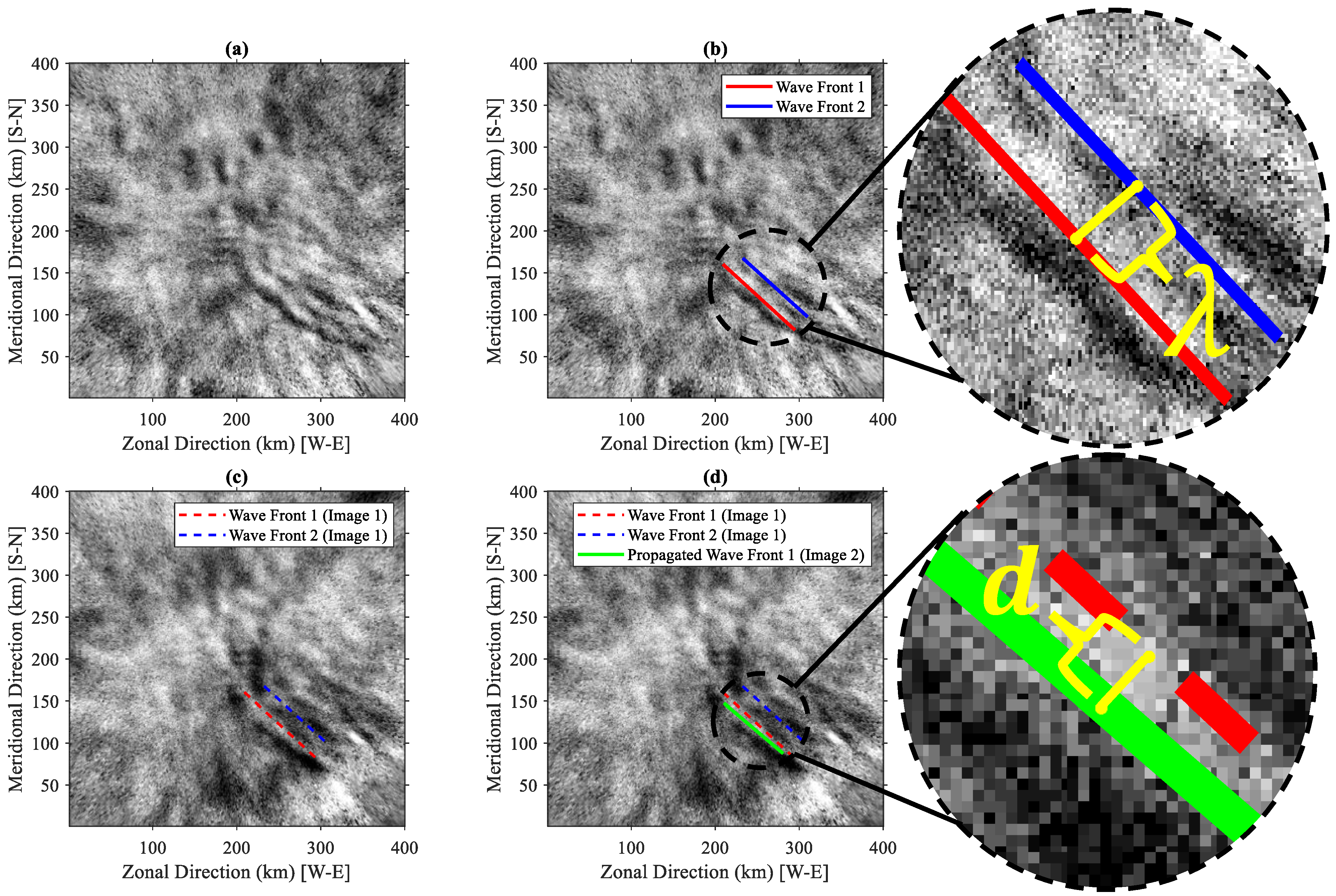
In Figure 5, two event analysis stages are concisely explained. It should be noted that Figure 5a and Figure 5b both represent the 1st AGW observation on 8 October 1998 at 10:10 UT. Similarly, Figure 5c and Figure 5d both represent the 2nd AGW observation on 8 October 1998 at 10:15 UT, where the time difference between the two AGW observations is 5 min. In the 1st AGW observation in Figure 5a, two consecutive wave fronts are selected by placing 5 points on each peak separately. In Figure 5b, least square fitting is used to draw two lines on each wave front using the preplaced points, where the red line represents wave front 1 and blue line represents wave front 2. The perpendicular distance between the red and blue lines with respect to their centers is used to calculate the wavelength (λ) as shown in the zoomed area next to Figure 5b.

In the 2nd AGW observation in Figure 5c, the two selected wave front lines appear to the left of those in Figure 5b. To indicate the wave propagation after a time-period (Δt) of 5 min, another 5 points were placed on the propagated wave front 1. In Figure 5d, least square fitting is used to draw the green line which represents the propagated wave front 1. The propagation distance/displacement ($\overrightarrow{d}$) is calculated by finding the perpendicular distance from the center of the green line to the center of the red line as indicated in the zoomed section next to Figure 5d.

Finally, the AGW propagation direction is calculated by finding the angle ϕ in degrees from the eastward direction, The angle is calculated based on the displacement vector in the meridional (${\overrightarrow{d}}_{\mathit{y}}$) and zonal (${\overrightarrow{d}}_{\mathit{x}}$) directions, which are represented by vertical and horizontal axes. Accordingly, the angle can be calculated similar to angle calculation in the cartesian coordinates from the positive x-axis which highlights the east direction. Regardless of the criteria in each quarter of the cartesian coordinates, the main equation governing the angle calculations is presented in Equation (3). However, AGW phase velocities in the zonal direction (v_zonal) and the meridional direction (v_meridional) are calculated by Equations (4) and (5). The equations seem to be very simple because of the projection advantage in geographical coordinates.

$$\begin{array}{c}\varphi =\tan \left(\left|{\displaystyle \frac{{\overrightarrow{d}}_y}{{\overrightarrow{d}}_x}}\right|\right) \end{array}$$

(3)

$$\begin{array}{c}{v}_{zonal}={\displaystyle \frac{\left|d\right|}{\Delta \mathrm{t}}}\cos \left(\varphi \right) \end{array}$$

(4)

$$\begin{array}{c}{v}_{meridional}={\displaystyle \frac{\left|d\right|}{\Delta \mathrm{t}}}\sin \left(\varphi \right) \end{array}$$

(5)

As most of the AGW observations are not simple wave structures to be distinguished by the event analysis, many complex wavefronts challenge the event analysis method and prevent extracting AGW phase velocities and direction accurately. The spectral analysis method becomes very important and essential in this case, where the AGW images are converted from the spatial domain to the frequency domain based on the 3-Dimensional Fast Fourier Transform (3-D FFT) method. However, from the spectral analysis, AGW dominant phase velocities and directions were calculated.

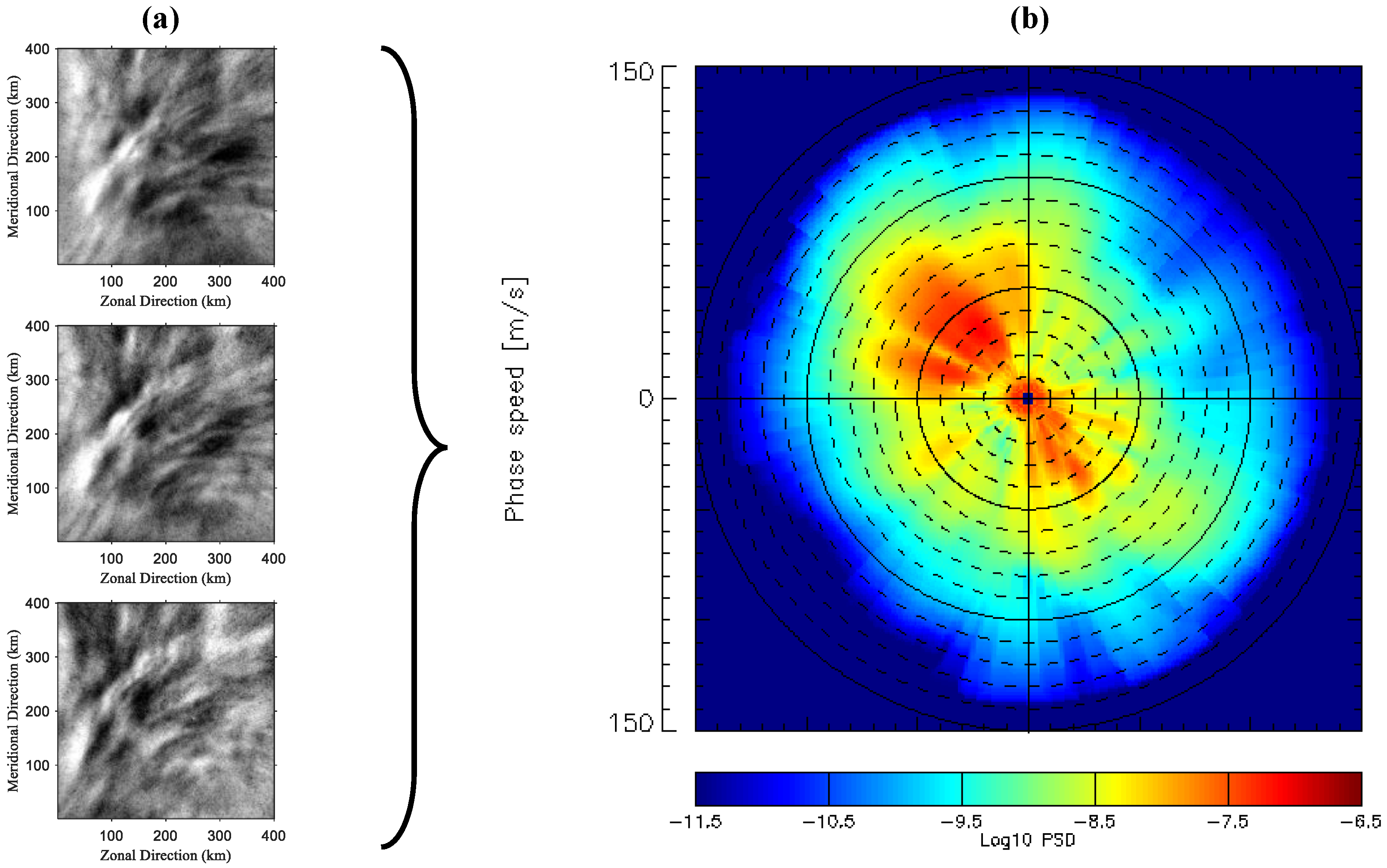
In Figure 6, three sequential AGW observations are prepared with an approximately fixed time difference to find phase velocities using spectral analysis according to Equations (6) and (7). The direction is calculated from the east (+x axis) similar to Equation (3), but involving zonal and meridional velocities instead of displacements.

$$\begin{array}{c}{v}_{zonal}={\displaystyle \frac{\omega k}{k^2+l^2}} \end{array}$$

(6)

$$\begin{array}{c}{v}_{meridional}={\displaystyle \frac{\omega l}{k^2+l^2}} \end{array}$$

(7)

where v_zonal, v_meridional, ω, k, l are the zonal velocity component, meridional velocity component, power spectrum frequency, zonal wave number, and meridional wave number, respectively. In Figure 6a, three sequential observations are presented to extract AGW phase velocities in the zonal and meridional directions, starting from date/time 24 October 2001 14:26 at the top and ending at date/time 24 October 2001 14:37 at the bottom. The result is computed in Figure 6b using 3-D FFT and presented in the log10 phase spectrum density scale from dark blue (−11.5) to dark red (−6.5). The dominant phase velocities in the zonal and meridional directions were determined from 3 to 5 consecutive images by integrating the horizontal velocity spectrum in the range of 20 to 150 m/s, where the spectrum range of 0 to 20 m/s was eliminated to avoid the contamination of white noise in airglow images.

Finally, the results of the two methods mentioned are regarded as numerical values of 1402 observations at a ~95 km altitude, where the data will be attributed to the training, validation, and testing phases of the machine learning approach based on a cascade forward neural network.

2.4. Cascade Forward Neural Network

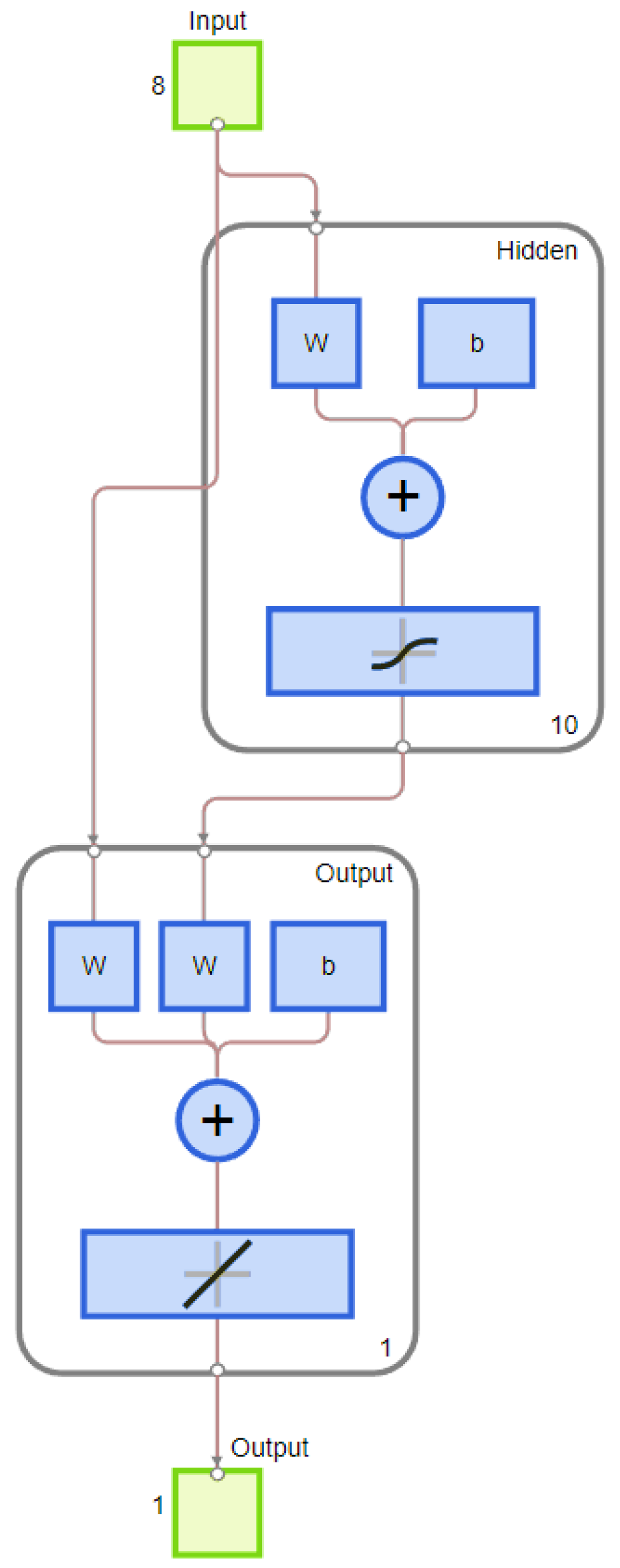
The cascade neural network (CFNN) is a distinct class from the feed-forward neural network (FFNN). A simple neural network (NN) contains computational elements called neurons, where each neuron represents a linear relationship between inputs and outputs. On the contrary, the simple structure of FFNN consists of three fundamental layers—input, hidden, and output—while a nonlinear relationship is introduced when a hidden layer is added to the simple system of neurons to convert the simple NN into an FFNN. In the hidden layer, an activation function is obtained to link the external input to the network’s output which enables the network to learn and complete complex tasks. Consequently, the output of the hidden layer is passed to the network’s output layer as a weighted sum, ensuring consistency in the transferred information. All information in FFNN moves in one direction (input layer → hidden layer → output layer). On the other hand, the input layer in CFNN is connected to both the hidden and output layers [10]; hence, its structure is shown in Figure 7.

The network is able to recognize the input–output correlation upon systematic adjustment of weights in the training phase. The input layer consists of an adjusted number of neurons, where each neuron relates to one considered variable, whereas the output layer contains a number of nodes based on the desired outputs. The observations provided to the network are equally distributed across the seasons but randomly selected by the network within each season, with a total of 1402 observations at an altitude of ~95 km. Consequently, these observations are divided into percentages of 70% (982 observations) in training, 15% (210 observations) in validation, and 15% (210 observations) in testing. In order to evaluate the network performance and dependability, both overtraining and undertraining were taken into consideration. Overtraining occurs when the network memorizes training data and produces deprived predictions/expectations, whereas undertraining is arises when the network estimates simplistic patterns that fail to capture the complexity of the provided dataset [39]. The CFNN deep neural network is introduced by the following equation.

$$\begin{array}{c}y={\displaystyle \sum _{i=1}^n}{f}^i\left({\omega }_i^i{x}_i\right)+f^0\left({\displaystyle \sum _{j=1}^m}{\omega }_j^0{f}_j^h\left({\displaystyle \sum _{a=1}^n}{\omega }_{aj}^h{x}_a\right)\right) \end{array}$$

(8)

where ${\omega }_i^i$ is the net input–output weight of one neuron y and f⁰ indicates the activation function. The input–hidden layer weights are denoted by ${\omega }_{aj}^h$; finally, the hidden layer activation function is $f_i^h$. The backpropagation training/optimization algorithm of Levenberg–Marquardt (LM) was implemented during the training phase [40,41]. The LM algorithm was chosen because of its fast convergence and low average absolute error [41,42], while ensuring updating of the weights based on Equation (9) [43].

$$\begin{array}{c}\Delta \omega ={\displaystyle \frac{1}{J^{T}J+\sigma I}}{J}^T\zeta \end{array}$$

(9)

According to Equation (9), Δω represents the weight’s errors, J is the Jacobian matrix, σ is a scalar, and the error vector is ζ. Nevertheless, the LM’s default gradient function is implemented to boost the speed in the training phase, Equation (10).

$$\begin{array}{c}\Delta \omega \left(\tau +1\right)=\psi \omega \left(\tau \right)-\rho {\displaystyle \frac{d\zeta }{d\omega }} \end{array}$$

(10)

In Equation (10), $\Delta \omega$ represents the errors per each weight, $\tau$ is the epoch, $\psi$ is the momentum parameter, and $\rho$ is the learning rate. To improve the per iteration training speed, $\rho$ should be corrected accordingly. The optimal performance of the CFNN was determined iteratively by selecting the number of neurons that yielded the lowest average Root Mean Square Error (RMSE) for both meridional and zonal velocity components as shown in Figure 8.

In the output layer, the Purelin function is employed as a linear transfer function. To introduce nonlinearity, the network employs a log-sigmoid function activation function, which defined by Equation (11).

$$\begin{array}{c}g\left(x\right)={\displaystyle \frac{1}{1+e^{-x}}} \end{array}$$

(11)

Accordingly, (x) is regarded as a matrix that defines the net input vectors. However, the network’s error is estimated by the cost function E in Equation (12).

$$\begin{array}{c}E={\displaystyle \frac{1}{n}}{\displaystyle \sum _{i=1}^n}\left(O^i-T^i\right) \end{array}$$

(12)

where n, O, and T are the overall training samples, the network’s output values, and the network’s target values, respectively. The estimation of this network performance is based on RMSE and the cross-correlation coefficient (R). The Root Mean Square Error (RMSE) is the square root of Equation (12) utilized to evaluate the difference between the estimated and observed meridional and zonal components of AGW observations, Nevertheless, the correlation coefficient (R) is defined based on Equation (13) and determines the closeness between the estimated and observed meridional and zonal components.

$$\begin{array}{c}R={\displaystyle \frac{\sum _{i-1}^n\left[\left(T^i-T\right)\left(O^i-O\right)\right]}{\sqrt{\sum _{i-1}^n{\left(T^i-\overline{T}\right)}^2}\sqrt{\sum _{i-1}^n(O^i-{\overline{O})}^2}}}\end{array}$$

(13)

However, the network can learn seasonality pattern, by defining midnight and year boundary continuity, both universal time (UT) and day of year (DOY) should be converted to a quadrature pair to help the neural network to distinguish that pattern, based on Equations (14)–(17) [44].

$$\begin{array}{c}\mathrm{DOYs}=\sin \left({\displaystyle \frac{2\pi \times \mathrm{D}\mathrm{O}\mathrm{Y}}{365.25}}\right) \end{array}$$

(14)

$$\begin{array}{c}\mathrm{DOYc}=\cos \left({\displaystyle \frac{2\pi \times \mathrm{D}\mathrm{O}\mathrm{Y}}{365.25}}\right) \end{array}$$

(15)

$$\begin{array}{c}\mathrm{UTs}=\sin \left({\displaystyle \frac{2\pi \times \mathrm{U}\mathrm{T}}{24}}\right) \end{array}$$

(16)

$$\begin{array}{c}\mathrm{UTc}=\cos \left({\displaystyle \frac{2\pi \times \mathrm{U}\mathrm{T}}{24}}\right) \end{array}$$

(17)

The training of the CFNN is based on 8 features in the input layer: wind meridional velocity, wind zonal velocity, wave phase meridional velocity, wave phase zonal velocity, wave dominant direction, and wind dominant direction, day of year sine component (DOYs), day of year cosine component (DOYc), universal time sine component (UTs), and universal time cosine component (UTc). In Figure 7, the number of input features is highlighted in the input layer, where the feature observations are obtained in the same data size and the same date/time of AGW phase velocities at a ~95 km altitude. Furthermore, to present the feature contribution (feature importance) of each neuron in the hidden layer, various approaches are introduced, such as connection weight, partial derivatives, input perturbation, and the Garson algorithm. According to a comparative study [45], the Garson algorithm commonly underestimates or overestimates feature importance values, while the rest were consistent with each other and the connection weight (CW) approach was the best.

Finally, feature importance was adopted based on the CW approach to find the feature parameters for each input-to-output contribution. The results were normalized to find the percentage of importance. Overall, this method is defined based on the importance weight Equation (18) of the input variable (neuron-i) and output variable (o), where the (input–output) neuron weight is w_io. The result is obtained from the sum of the products of connection weights, namely (input–hidden) w_ih and (hidden–output) neuron connection weight v_ho, where the hidden neuron is h and the hidden neuron number is n [46].

$$\begin{array}{c} w_{io}={\displaystyle \sum _{h=1}^n}{w}_{ih}{v}_{ho} \end{array}$$

(18)

2.5. Physics-Guided Database

Unlike physics-guided neural networks which are considered as NNs that learn the physics of specific phenomena from training datasets obtained by physics data-driven techniques under certain physics-based constraints and loss functions [47], in this study CFNN is data-driven [48] but trained on a physics-guided database, which is determined from physics-based approaches to ensure that the network exhibits physical consistency from the data input. As an illustration, AGW phase velocity and direction parameters are calculated using the event and spectral analysis methods. Nevertheless, neutral wind data parameters in the zonal and meridional directions were obtained from MU radar and HWM. The MU radar is a meteor radar which indirectly measures the wind velocities based on meteor echo distribution under Doppler and geometry constraints [23], while HWM is guided by empirical physics-based models of thermosphere wind. In HWM, wind velocities are governed by Equations (19) and (21) as well as Relation (20) [24].

$$\begin{array}{c}U\left(\tau ,\delta ,\theta ,\varphi \right)={\displaystyle \sum _J}{\beta }_j\left(z\right)u_j\left(\tau ,\delta ,\theta ,\varphi \right) \end{array}$$

(19)

where $U\left(\tau ,\delta ,\theta ,\varphi \right)$ is the zonal wind component, ${\beta }_j\left(z\right)$ is the amplitude of the j-th vertical kernel, $u_j\left(\tau ,\delta ,\theta ,\varphi \right)$ is the periodic horizontal spatiotemporal variations for the j-th vertical kernel, $\tau$ is the day of year, $\delta$ is the solar local time, $\theta$ is the colatitude, and $\varphi$ is the longitude.

However, the meridional wind component $v_j\left(\tau ,\delta ,\theta ,\varphi \right)$ is extracted from the same formulation as the zonal component using the vector spherical parity relation (20).

$$\begin{array}{c}u :\left\{C_r,C_i,B_r,B_i\right\} \leftrightarrow -v : \left\{B_r,B_i,-C_r,-C_i\right\} \end{array}$$

(20)

$C_r, C_i, B_r$, and $B_i$ represent the real and imaginary parts of the vorticity and divergence of the vector wind field.

Along a particle geographic bearing ($\varphi$), the line-of-sight wind ($w_{los}$) is expressed by Equation (21) using a linear basis that includes a zonal wind component ($u$) and a meridional wind component ($v$).

$$\begin{array}{c}{w}_{los}=u\sin \left(\varphi \right)+v\cos \left(\varphi \right) \end{array}$$

(21)

Finally, the direction of neutral wind was obtained from the meridional and zonal velocity components, where the year and midnight boundaries are calculated according to Equations (14)–(17) to help the CFNN to learn and recognize the seasonal pattern.

3. Results and Discussion

3.1. Convolutional Neural Network Classification

Classification has been achieved in all proposed networks. They are trained by 10,813 images and tested by 1194 images; all images are classified into two classes (GW and NGW). In the training and validation phases, the GW class contains 7516 images arranged sequentially and distributed over the years from October 1998 to October 2002. On the other hand, the NGW class contains 3297 images. In the testing phase, the GW class contains 831 images, and the NGW class contains 363 images. In Figure 9, accuracy and loss during the training and validation phases are presented for AlexNet in Figure 9a, GoogLeNet in Figure 9b, and ResNet-50 in Figure 9c. However, the loss was implemented to measure the difference between predicted and expected outcomes, where the loss function is very useful to optimize the network parameters by reducing that difference [49].

In the training and validation phases, AlexNet is considered as the best-performing deep neural network with the highest training and validation accuracies and the least validation loss and time consumption, as summarized in

Table 3. Summary to the best performance of all deep neural networks in the training and validation phases.

Network	Time hh:mm:ss	Epoch	Training Accuracy	Validation Accuracy	Training Loss	Validation Loss
AlexNet	00:07:05	16	100%	99.26%	0.0011	0.0206
GoogLeNet	00:22:47	16	100%	98.80%	0.0069	0.0359
ResNet-50	03:27:55	16	100%	98.61%	0.0056	0.0467

at epoch 16.

Next we sought further clarification regarding the validation accuracy during the training phase, which should be considered after stabilization. Accordingly, stabilization has approximately occurred after epoch 1, where the validation frequency is considered per every 50 iterations. The ANOVA analysis and Tukey test were conducted using ORIGIN software (version 2025). According to ANOVA analysis, the mean of the validation accuracy, in addition to the F-statistic value (~49.8) and p-value (<0.0001), collectively support that AlexNet is the best-performing deep neural network during the training phase. The supporting data are summarized in

Table 4. Summary of ANOVA analysis results.

Network	N	Mean	Standard Deviation	Tukey Test
AlexNet	46	~99.12%	~0.216	A
GoogLeNet	46	~98.40%	~0.501	B
ResNet-50	46	~97.96%	~0.813	C

, where the number of samples (N), mean of validation accuracy (Mean), standard deviation, and Tukey test are shown for all three networks. Moreover, the Tukey test ensures that the means that do not share a letter are significantly different. However, the best network will be chosen and determined after the testing phase.

The confusion matrices are presented in Figure 10, where accuracy and precision percentages are calculated based on Equations (1) and (2). However, each matrix is divided into four corners; the top left is true positive (TP), the bottom right is true negative (TN), the bottom left is false positive (FP), and the top right is false negative (FN). In the testing phase, the accuracy and precision for AlexNet in Figure 10a are 98.41% and 98.33%, for GoogLeNet in Figure 10b they are 98.24% and 98.45%, and for ResNet-50 in Figure 10c they are 97.91% and 98.21%, respectively.

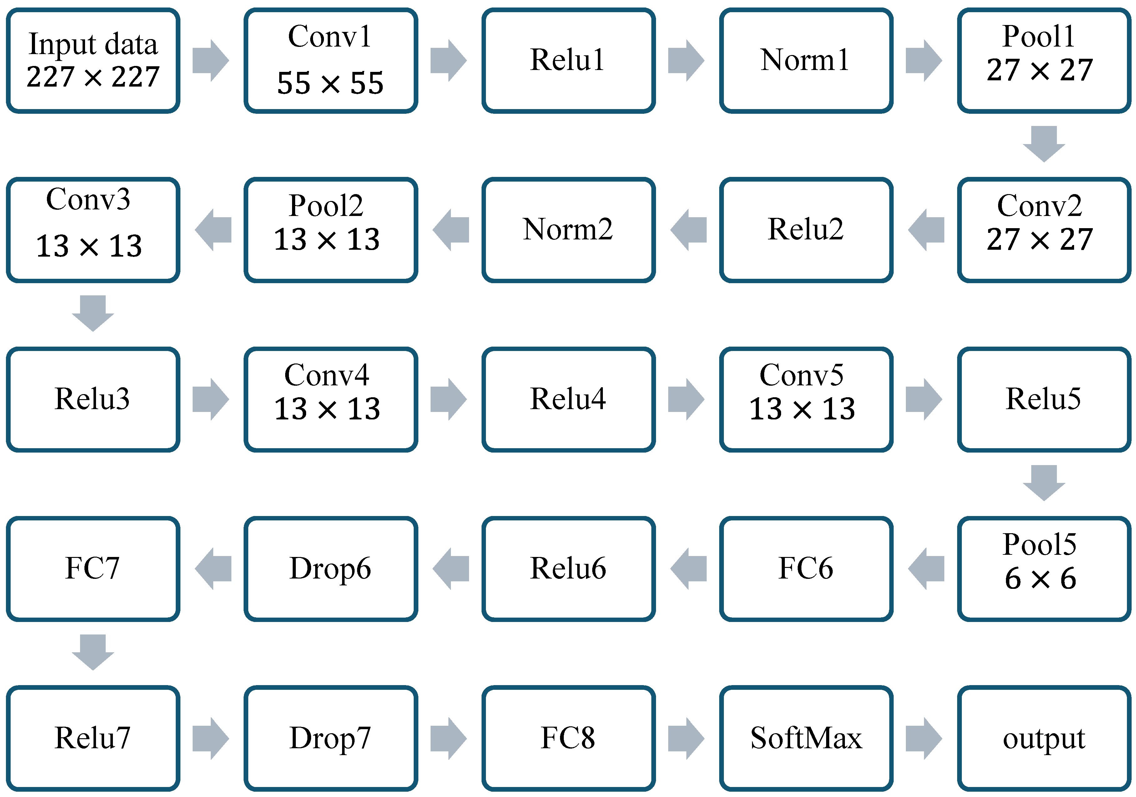
Finally, AlexNet was indicated as the best-performing deep neural network in the testing phase, which makes it ideal for classifying AGW images in projected geographic coordinates. The structure of AlexNet is presented in Figure 11. Briefly, it contains five convolutional (Conv) layers, seven rectifying linear units (ReLU), two response normalization (norm) layers that ensure learning generalization across neurons, three pooling (pool) layers were used for down-sampling while progressing through the layers, three fully connected (FC) layers, the output of the last fully connected (FC) layer going to a two-way SoftMax which generates the distribution over an equivalent number of class labels, and two dropout layers that reduce test errors, preventing overtraining and contributing to the final network’s decision. The full coverage of the network is covered by Krizhevsky [30].

3.2. Cascade Forward Neural Network Regression

The extracted features were considered for MU radar and HWM to highlight the zonal and meridional wind velocities; from these velocities, the dominant wind directions were calculated in a similar manner to AGW directions, which is stated in the event and spectral methods sections. However, based on the dominant zonal and meridional AGW phase velocities that were extracted by event and spectral analysis methods, the dominant AGW direction was calculated at each date/time that was provided by the extracted image sequence. To ensure seasonal continuity, the DOY and UT components were calculated based on each date/time provided by each image sequence according to Equations (14)–(17). All features are organized to find a hidden correlation between them and the target values of AGW phase velocities in the meridional and zonal directions. The aim of this work is to estimate/predict the atmospheric gravity wave phase velocities in the mesosphere region at a ~95 km altitude. Based on the estimated values, the AGW horizontal phase speeds and dominant directions in the mesosphere region are calculated per season, where AGW phase velocities are treated as response parameters that could be estimated by the CFNN.

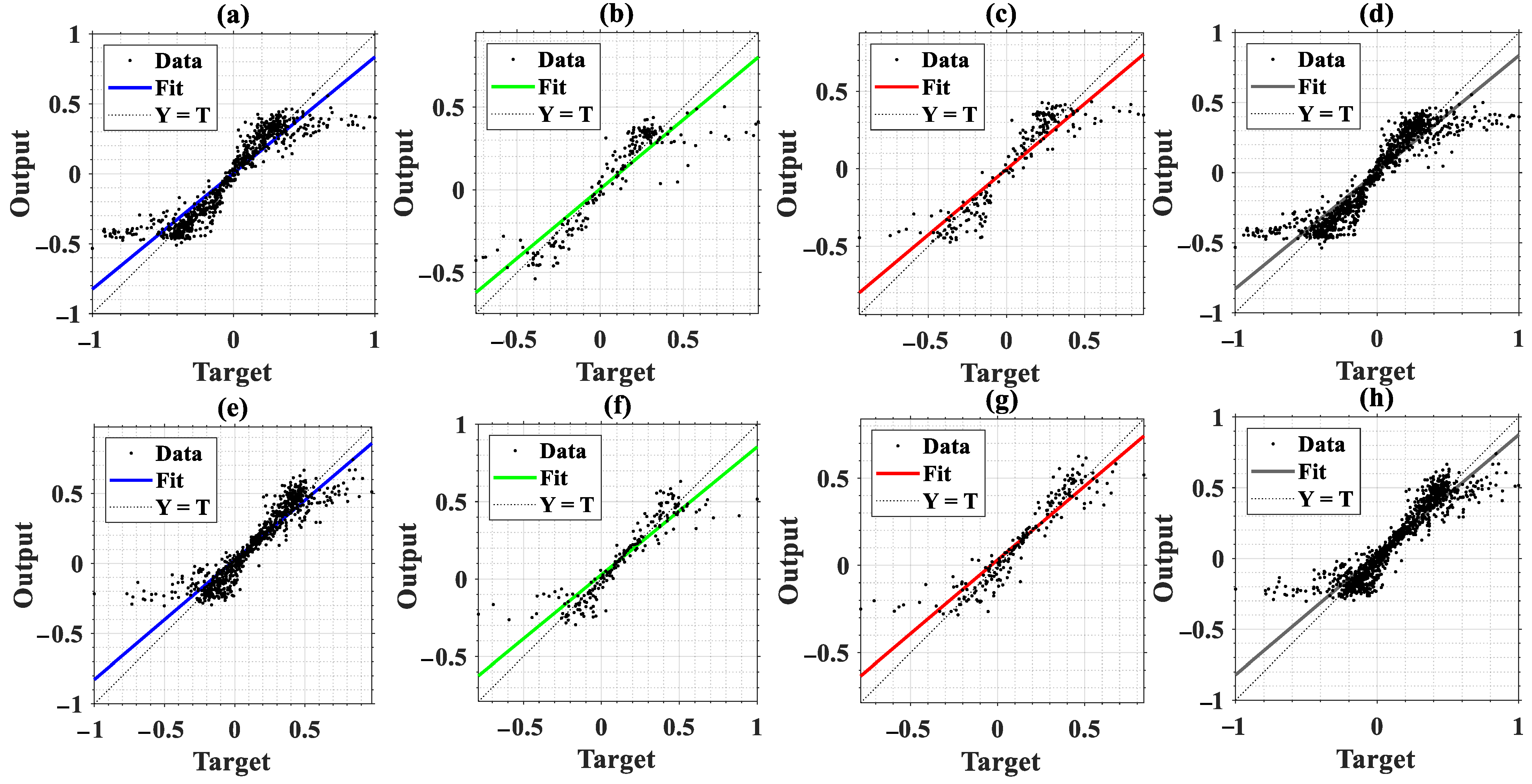
The data has been fed to the network, where each AGW phase velocity component in the meridional and zonal directions is subjected to the network separately from each other. In Figure 12, the network’s estimated values are regarded as the “output”, while the observed values are treated as the “target”. The phases of training, validation, testing, and overall performance are presented for the AGW meridional component from Figure 12a to Figure 12e, as well as the AGW zonal component from Figure 12e to Figure 12h, respectively. The correlation coefficient (R) of AGW meridional velocity was a little higher than that of AGW zonal velocity in each corresponding phase. Nonetheless, meridional and zonal AGW velocities had R values greater than 0.90 in all phases, except in the validation phase of the AGW zonal velocity which was slightly lower and given by ~0.897.

To ensure that the network was not overtrained or undertrained, CFNN was automatized to keep track of the best performance. During the training process, CFNN was adjusted at the epoch that corresponded to the lowest mean square error (MSE) value. However, exceeding this epoch might produce undesired results which correspond to overtraining.

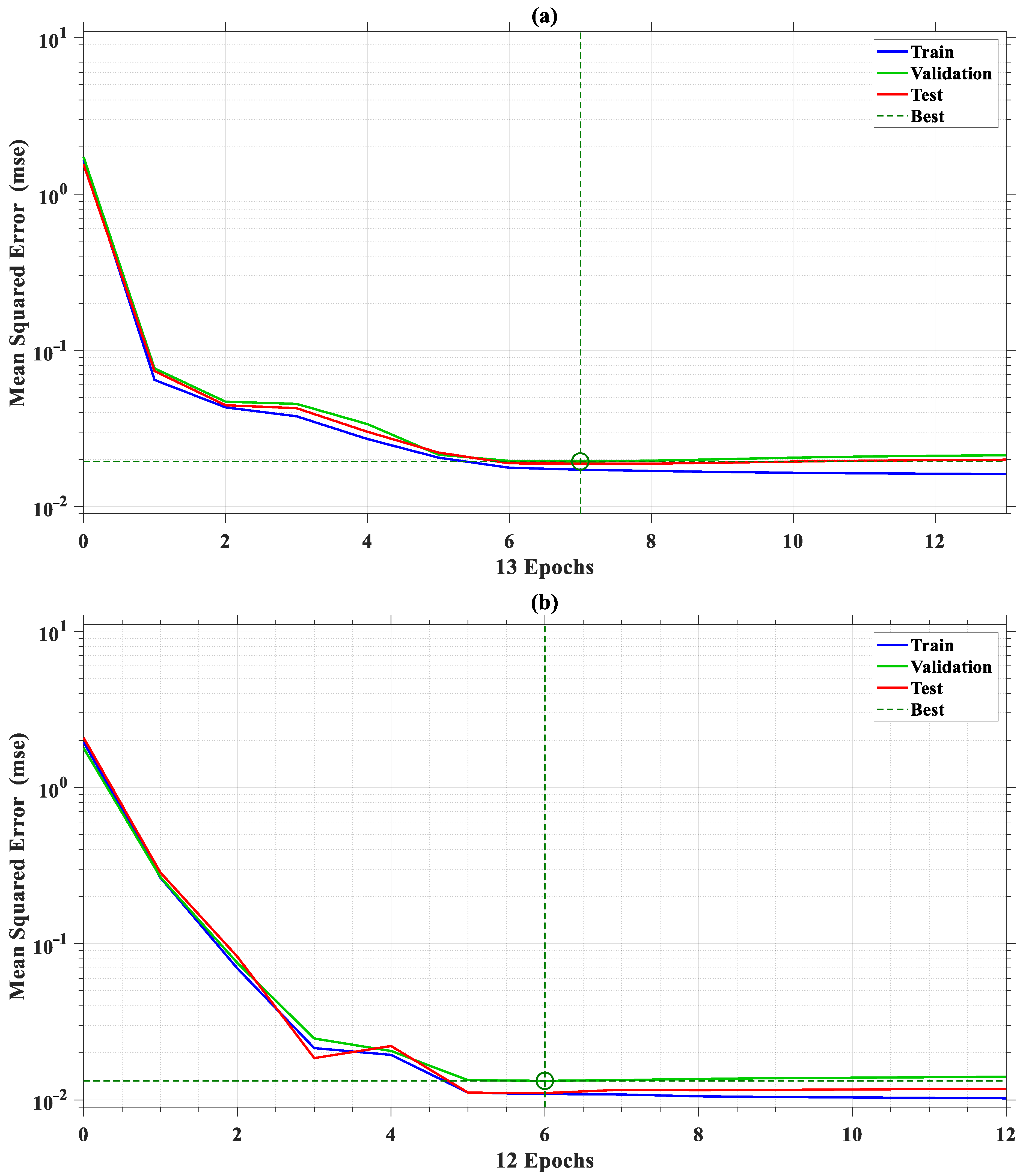
In Figure 13, the best validation performance for the AGW meridional and zonal phase velocities resulted in the lowest MSE ~0.019417 and ~0.013242 at epochs 7 and 6 in Figure 13a,b, respectively.

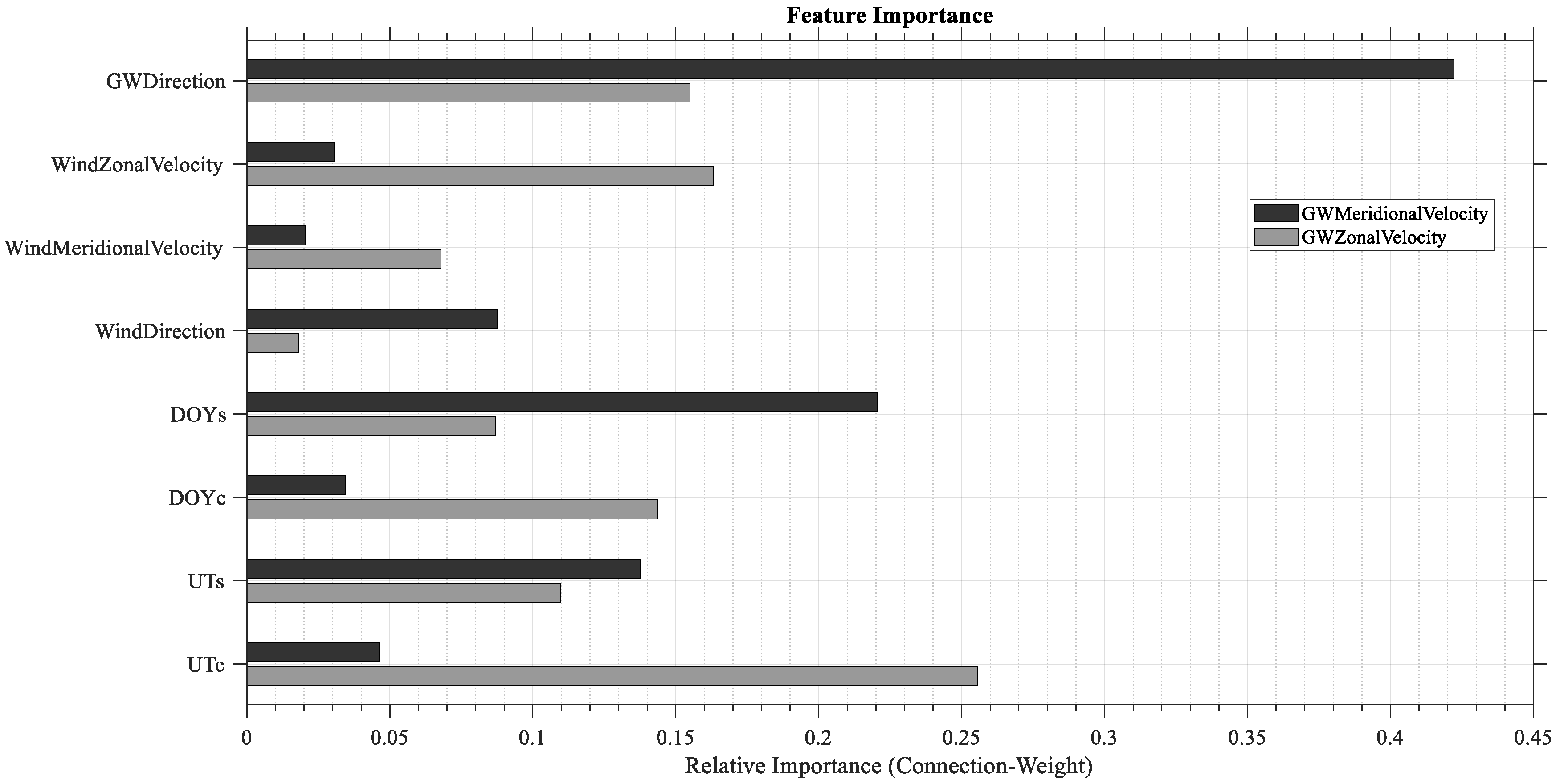
Regarding each feature parameter fed to the network, the relative importance of AGW phase velocities in the meridional and zonal directions is presented in Figure 14.

The dependence of the AGW meridional and zonal velocities was ranked based on the relative importance of the connection weight method as presented in

Table 5. Feature importance ranking.

Rank	AGW Meridional Velocity Component	Percentage (%)	AGW Zonal Velocity Component	Percentage (%)
1	Gravity Wave Direction	42.22	Cosine Component of Universal Time	25.55
2	Sine Component of Day of Year	22.06	Neutral Zonal Wind Velocity	16.32
3	Sine Component of Universal Time	13.75	Gravity Wave Direction	15.51
4	Neutral Wind Direction	8.77	Cosine Component of Day of Year	14.34
5	Cosine Component of Universal Time	4.63	Sine Component of Universal Time	10.98
6	Cosine Component of Day of Year	3.46	Sine Component of Day of Year	8.71
7	Neutral Zonal Wind Velocity	3.07	Neutral Meridional Wind Velocity	6.79
8	Neutral Meridional Wind Velocity	2.04	Neutral Wind Direction	1.81

. The best parameters used by CFNN to estimate the AGW meridional velocity were the AGW propagation direction and seasonality sine components, as well as neutral wind direction, with a percentage higher than 8%. On the contrary, the best parameters contributing to the estimation of the AGW zonal velocity were seasonality cosine components, neutral zonal wind velocity, and AGW propagation direction, with a percentage greater than 10%.

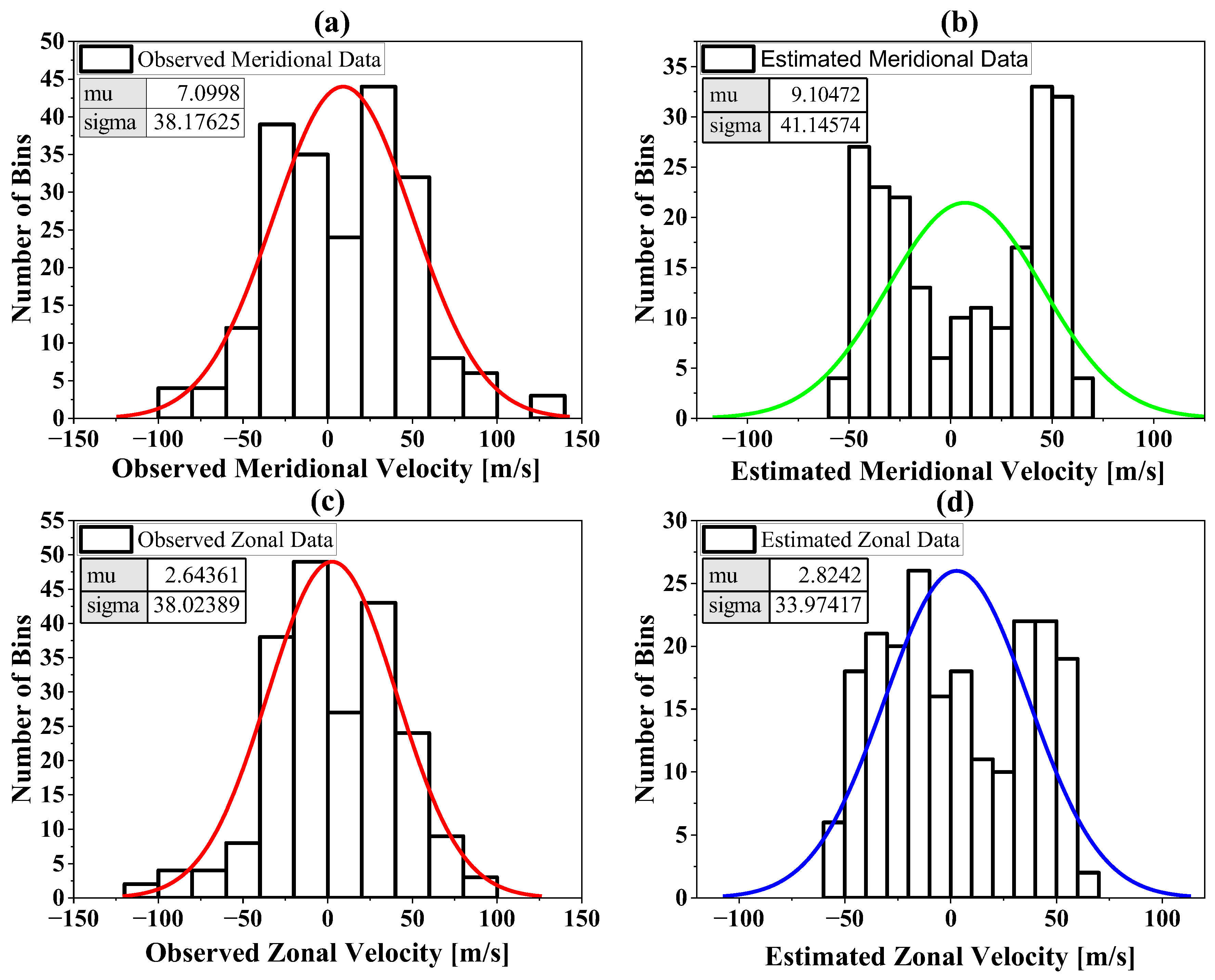
The Gaussian normal distribution of velocity data in all seasons regarding the testing phase is expressed in Figure 15. Each subfigure contains two values: the mean shown as mu (μ) and standard deviation (SD) shown as sigma (σ). In Figure 15a,b, the observed and estimated meridional components were presented; their means are ~7 m/s and ~9 m/s, and their SDs are ~38 m/s and ~41 m/s. In Figure 15c,d, the observed and estimated zonal components were presented; their means are ~3 m/s and ~3 m/s, and their SDs are ~38 m/s and ~34 m/s. However, the SD shows the velocity distribution about the respective mean value. In Figure 15a, the observed meridional velocity is distributed over ±38 m/s about the central mean of ~7 m/s, which approximately gives the meridional velocity distribution from –31 m/s to +45 m/s. In Figure 15b, the estimated meridional velocity distribution is from −32 m/s to +50 m/s about a central mean of ~9 m/s. In Figure 15c, the observed zonal velocity distribution is from −35 m/s to +41 m/s about a central mean of ~3 m/s. In Figure 15d, the estimated zonal distribution is from −31 m/s to +37 m/s about a central mean of ~3 m/s. Accordingly, the distribution of estimated phase velocities in the testing phase is close to the observed values.

Based on the existing studies [11,50,51], the dominant horizontal phase speeds and directions are presented over Shigaraki per season: in spring, they range from ~45 to ~70 m/s directed northeastward; in summer, from ~45 to ~70 m/s directed north and northeastward; in fall, from ~40 to ~60 m/s directed northwestward; and in winter, from~40 to ~50 m/s directed southwestward, respectively. Accordingly, the dominant phase speeds calculated per season based on the phase velocities estimated by the network are highlighted. In spring, they range from ~45 to ~55 m/s; in summer, from ~50 to 60 m/s; in fall, from ~50 to ~60 m/s; and in winter, from ~40 to ~60. Despite the accuracy of the results in spring, summer, and fall, around 36% of the dominant horizontal phase speeds were overestimated by a difference of ~10 m/s in winter with respect to the maximum velocity illustrated by the existing studies, which makes the network less accurate in that season.

However, the overestimation performed by CFNN in winter can be explained using Figure 1 and Table 5; the number of AGW observational hours in winter is higher than the other three seasons as shown in the figure, while according to the feature ranking table, the zonal wind velocity ranks as the second most important factor influencing the AGW velocity estimation in the zonal direction using the CFNN, which in turn affects the overall estimated dominant velocity range of AGWs. Accordingly, the number of observations in the winter was the largest among all seasons and the average neutral zonal wind velocity was the highest as well. However, the standard deviation of zonal wind velocity in winter was considered as the second-largest deviation after spring, which suggests strong variability in winter’s zonal velocity data. Overall, this may have biased the CFNN toward being more likely to estimate higher velocities for AGWs in winter, which has been achieved by assigning larger connection weights that effectively increased the probability of favoring higher zonal wind velocities during the training phase.

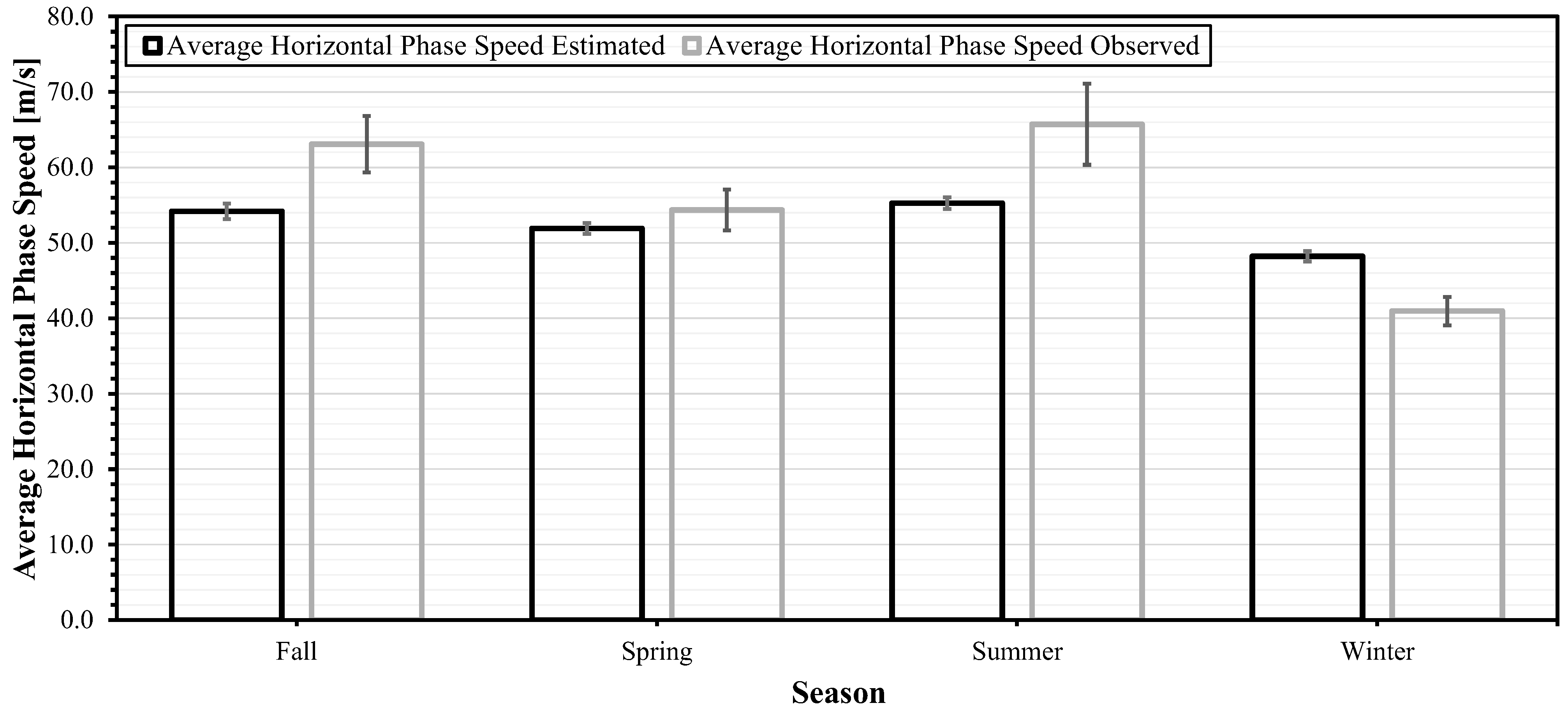
The average horizontal phase speed calculated based on the estimated AGW phase velocities by CFNN in the meridional and zonal directions is called the horizontal phase speed estimated (HPSE). On the other hand, the average horizontal phase speed calculated based on the observed AGW phase velocities by event and spectral methods is called the horizontal phase speed observed (HPSO). Moreover, each average horizontal phase speed is calculated per season and presented depending on the CFNN data in the testing phase.

In Figure 16, HPSE is plotted in comparison to HPSO per season and shown in black and gray colors, respectively. The error bars are the standard error in the testing dataset per season. The HPSE values in fall, spring, summer, and winter are 54.2 ± 1.0, 51.9 ± 0.7, 55.3 ± 0.8, and 48.2 ± 0.7 m/s, respectively. Similarly, the HPSO values are 63.1 ± 3.8, 54.3 ± 2.7, 65.7 ± 5.4, and 41.0 ± 1.9 m/s, respectively. HPSE is closer to HPSO in spring and winter than in fall and summer.

Previously, the network performed very well in estimating AGW velocities and horizontal phase speeds; another test was performed to investigate whether the network can distinguish directions correctly. In Figure 17, the directions are presented per season based on the estimated AGW phase velocities by CFNN in the zonal and meridional components, where the scale presented in each plot is the percentage per direction, which can be calculated by dividing the number of observations in a specific direction by the total number of observations of its respective season. The octants criteria for dividing directions per season into eight components adhered to Waltersceid [52]. In this study, the dominant directions E, NE, N, NW, W, SW, S, and SE are presented with the angle range in degrees as east (337.5 to 22.5°), northeast (22.5 to 67.5°), north (67.5 to 112.5°), northwest (112.5 to 157.5°), west (157.5 to 202.5°), southwest (202.5 to 247.5°), south (247.5 to 292.5°), and southeast (292.5 to 337.5°).

In Figure 17A, the estimated propagation direction of AGWs in fall was north and northwestward, both equally given by the largest percentage of 22.5%. In Figure 17B, the dominant direction in summer is north and northeastward, with the largest percentage of 34.375% each. In Figure 17C, the dominant direction in spring is northeastward with 22.5%. In Figure 17D, the dominant direction in winter is south with 23.2% and southwestward with 22.2%.

4. Conclusions

In atmospheric gravity wave research, specifically when it comes to investigating AGW phenomena observed by ASAI in the mesosphere region, the process of classifying a large dataset of images by “visual inspection” is gigantically time-consuming and might lead to biased results.

In this article, three CNNs were introduced to recognize the AGW signatures in images from OI 557.7 nm ASAI. The captured images with OI-Filter 557.7 nm are enhanced deviated images projected in geographic coordinates, and these images were classified into two separate classes (gravity waves and non-gravity waves). After the testing phase, the accuracy and precision for AlexNet were 98.41% and 98.33%, for GoogLeNet they were 98.24 and 98.45%, and for ResNet-50 they were 97.91% and 98.21%, respectively. Accordingly, the least time-consuming and most accurate neural network was AlexNet in comparison to the other proposed CNNs.

The CFNNs were trained using eight features to estimate the AGW phase velocities in the meridional and zonal directions, separately. In the validation and testing phases, the AGW meridional phase velocity correlation coefficients were 0.90833 and 0.92484, respectively, while the correlation coefficients regarding zonal velocity were 0.89673 and 0.90525, respectively.

The correlation results ensure a high correlation between the observed and estimated AGW phase velocities by CFNN. The average horizontal phase speeds and directions are presented in fall, spring, summer, and winter. Consequently, the results are given by ~54.2 m/s north and northwestward, ~51.9 m/s north and northeastward, ~55.3 m/s northeastward, and ~48.2 m/s south and southwestward, respectively. Nevertheless, AGW phase velocity distribution emphasizes a promising velocity forecast for the AGWs in the mesosphere region per season from October 1998 to October 2002.

In comparison with the existing studies, the dominant horizontal phase speed calculations were less accurate in winter. In the testing phase, the overall results depicted consistency with the existing studies regarding velocity distributions, horizontal phase speeds, and dominant directions. The network overestimated ~36% of dominant horizontal phase speeds from 50 m/s to 60 m/s, where the typical range is from 40 m/s to 50 m/s.

The limitations of CNN and CFNN utilized in this work must be acknowledged. CNNs require enhanced airglow images projected in geographical coordinates, while providing non-enhanced and non-projected images might lead to potential errors or inaccuracies. Similarly, phase velocity estimations by CFNN are regarded as spatially dependent and from one filter type, where the considered airglow images are from OI-Filter 557.7 nm ASAIs located at Shigaraki station. The CFNN, relied on a physics-based data-driven approach, has shown high performance in estimating/predicting AGW phase velocities, where more investigation is needed in different levels of solar activity, as well as estimating other parameters such as wavelengths.

However, the careful selection of the feature parameters for estimating AGW phase velocities ensures that the AGWs can be subjected to velocity forecasting in the mesosphere layer, which is helpful in investigating the cause–effect relationship between mesospheric gravity waves and plasma bubble events in the ionosphere [53], as well as traveling ionospheric disturbance

Finally, future work might integrate physics-informed neural networks under certain physical restrictions to improve generalization and physics-based interpretation.

References

1. Hines, C.O. Internal Atmospheric Gravity Waves at Ionospheric Heights. Can. J. Phys. 1960, 38, 1441–1481. [Google Scholar] [CrossRef]
2. Hecht, J.H.; Walterscheid, R.L.; Vincent, R.A. Airglow Observations of Dynamical (Wind Shear-induced) Instabilities over Adelaide, Australia, Associated with Atmospheric Gravity Waves. J. Geophys. Res. Atmos. 2001, 106, 28189–28197. [Google Scholar] [CrossRef]
3. Taylor, M.J.; Ryan, E.H.; Tuan, T.F.; Edwards, R. Evidence of Preferential Directions for Gravity Wave Propagation Due to Wind Filtering in the Middle Atmosphere. J. Geophys. Res. Space Phys. 1993, 98, 6047–6057. [Google Scholar] [CrossRef]
4. Lindzen, R.S. Turbulence and Stress Owing to Gravity Wave and Tidal Breakdown. J. Geophys. Res. Oceans 1981, 86, 9707–9714. [Google Scholar] [CrossRef]
5. Fritts, D.C. Shear Excitation of Atmospheric Gravity Waves. J. Atmos. Sci. 1982, 39, 1936–1952. [Google Scholar] [CrossRef]
6. Fritts, D.C. Gravity Wave Saturation in the Middle Atmosphere: A Review of Theory and Observations. Rev. Geophys. 1984, 22, 275–308. [Google Scholar] [CrossRef]
7. Taylor, M.J. A review of advances in imaging techniques for measuring short period gravity waves in the mesosphere and lower thermosphere. Adv. Space Res. 1997, 19, 667–676. [Google Scholar] [CrossRef]
8. Fritts, D.C.; Alexander, M.J. Gravity Wave Dynamics and Effects in the Middle Atmosphere. Rev. Geophys. 2003, 41, 1003. [Google Scholar] [CrossRef]
9. Krichen, M. Convolutional Neural Networks: A Survey. Computers 2023, 12, 151. [Google Scholar] [CrossRef]
10. Warsito, B.; Santoso, R.; Suparti; Yasin, H. Cascade Forward Neural Network for Time Series Prediction. J. Phys. Conf. Ser. 2018, 1025, 012097. [Google Scholar] [CrossRef]
11. Ejiri, M.K.; Shiokawa, K.; Ogawa, T.; Igarashi, K.; Nakamura, T.; Tsuda, T. Statistical Study of Short-Period Gravity Waves on OH and OI Nightglow Images at Two Separated Sites. J. Geophys. Res. Atmos. 2003, 108, 4679. [Google Scholar] [CrossRef]
12. Wrasse, C.M.; Nakamura, T.; Takahashi, H.; Medeiros, A.F.; Taylor, M.J.; Gobbi, D.; Denardini, C.M.; Fechine, J.; Buriti, R.A.; Salatun, A.; et al. Mesospheric Gravity Waves Observed near Equatorial and Low–Middle Latitude Stations: Wave Characteristics and Reverse Ray Tracing Results. Ann. Geophys. 2006, 24, 3229–3240. [Google Scholar] [CrossRef]
13. Mukherjee, G.K. The Signature of Short-Period Gravity Waves Imaged in the OI and near Infrared OH Nightglow Emissions over Panhala. J. Atmos. Sol. Terr. Phys. 2003, 65, 1329–1335. [Google Scholar] [CrossRef]
14. Kam, H.; Jee, G.; Kim, Y.; Ham, Y.; Song, I.-S. Statistical Analysis of Mesospheric Gravity Waves over King Sejong Station, Antarctica (62.2° S, 58.8° W). J. Atmos. Sol. Terr. Phys. 2017, 155, 86–94. [Google Scholar] [CrossRef]
15. Huang, H.; Gu, S.; Qin, Y.; Li, G.; Yang, Z.; Wei, Y.; Gong, D.; Niu, S. Statistical Analysis of Gravity Waves in the Mesopause Region Based on OI 557.7 Nm Airglow Observation over Mohe, China. J. Geophys. Res. Space Phys. 2025, 130, e2025JA033917. [Google Scholar] [CrossRef]
16. Hwang, J.-Y.; Lee, Y.-S.; Kim, Y.H.; Kam, H.; Song, S.-M.; Kwak, Y.-S.; Yang, T.-Y. Propagating Characteristics of Mesospheric Gravity Waves Observed by an OI 557.7 Nm Airglow All-Sky Camera at Mt. Bohyun (36.2° N, 128.9° E). Ann. Geophys. 2022, 40, 247–257. [Google Scholar] [CrossRef]
17. Matsuoka, D.; Watanabe, S.; Sato, K.; Kawazoe, S.; Yu, W.; Easterbrook, S. Application of Deep Learning to Estimate Atmospheric Gravity Wave Parameters in Reanalysis Data Sets. Geophys. Res. Lett. 2020, 47, e2020GL089436. [Google Scholar] [CrossRef]
18. Wu, Y.; Sheng, Z.; Zuo, X. Application of Deep Learning to Estimate Stratospheric Gravity Wave Potential Energy. Earth Planet. Phys. 2022, 6, 70–82. [Google Scholar] [CrossRef]
19. Amiramjadi, M.; Plougonven, R.; Mohebalhojeh, A.R.; Mirzaei, M. Using Machine Learning to Estimate Nonorographic Gravity Wave Characteristics at Source Levels. J. Atmos. Sci. 2023, 80, 419–440. [Google Scholar] [CrossRef]
20. Connelly, D.S.; Gerber, E.P. Regression Forest Approaches to Gravity Wave Parameterization for Climate Projection. J. Adv. Model. Earth Syst. 2024, 16, e2023MS004184. [Google Scholar] [CrossRef]
21. Lai, C.; Xu, J.; Yue, J.; Yuan, W.; Liu, X.; Li, W.; Li, Q. Automatic Extraction of Gravity Waves from All-Sky Airglow Image Based on Machine Learning. Remote Sens 2019, 11, 1516. [Google Scholar] [CrossRef]
22. Shiokawa, K.; Katoh, Y.; Satoh, M.; Ejiri, M.K.; Ogawa, T.; Nakamura, T.; Tsuda, T.; Wiens, R.H. Development of Optical Mesosphere Thermosphere Imagers (OMTI). Earth Planets Space 1999, 51, 887–896. [Google Scholar] [CrossRef]
23. Nakamura, T.; Tsuda, T.; Tsutsumi, M.; Kita, K.; Uehara, T.; Kato, S.; Fukao, S. Meteor Wind Observations with the MU Radar. Radio. Sci. 1991, 26, 857–869. [Google Scholar] [CrossRef]
24. Drob, D.P.; Emmert, J.T.; Meriwether, J.W.; Makela, J.J.; Doornbos, E.; Conde, M.; Hernandez, G.; Noto, J.; Zawdie, K.A.; McDonald, S.E.; et al. An Update to the Horizontal Wind Model (HWM): The Quiet Time Thermosphere. Earth Space Sci. 2015, 2, 301–319. [Google Scholar] [CrossRef]
25. Nakamura, T.; Higashikawa, A.; Tsuda, T.; Matsushita, Y. Seasonal Variations of Gravity Wave Structures in OH Airglow with a CCD Imager at Shigaraki. Earth Planets Space 1999, 51, 897–906. [Google Scholar] [CrossRef]
26. Kubota’, M.; Ishii’, M.; Shiokawa’, K.; Ejiri, M.K.; Ogawa, T. Height measurements of nightglow structures observed by all-sky imagers. Adv. Space Res. 1999, 24, 593–596. [Google Scholar] [CrossRef]
27. LeCun, Y.; Bengio, Y. Convolutional Networks for Images, Speech, and Time Series. Handb. Brain Theory Neural Netw. 1995, 3361, 1995. [Google Scholar]
28. Lecun, Y.; Bottou, L.; Bengio, Y.; Haffner, P. Gradient-Based Learning Applied to Document Recognition. Proc. IEEE 1998, 86, 2278–2324. [Google Scholar] [CrossRef]
29. Mittal, N. Automatic Contrast Enhancement of Low Contrast Images Using MATLAB. Int. J. Adv. Res. Comput. Sci. 2012, 3, 335–336. [Google Scholar]
30. Krizhevsky, A.; Sutskever, I.; Hinton, G.E. ImageNet Classification with Deep Convolutional Neural Networks. Commun. ACM 2017, 60, 84–90. [Google Scholar] [CrossRef]
31. Goodfellow, I.; Bengio, Y.; Courville, A. Deep Learning; MIT Press: Cambridge, UK, 2016. [Google Scholar]
32. Yamashita, R.; Nishio, M.; Do, R.K.G.; Togashi, K. Convolutional Neural Networks: An Overview and Application in Radiology. Insights Imaging 2018, 9, 611–629. [Google Scholar] [CrossRef] [PubMed]
33. Szegedy, C.; Liu, W.; Jia, Y.; Sermanet, P.; Reed, S.; Anguelov, D.; Erhan, D.; Vanhoucke, V.; Rabinovich, A. Going Deeper with Convolutions. In Proceedings of the IEEE Conference on Computer Vision and Pattern Recognition, Boston, MA, USA, 7–12 June 2015; pp. 1–9. [Google Scholar]
34. He, K.; Zhang, X.; Ren, S.; Sun, J. Deep Residual Learning for Image Recognition. In Proceedings of the IEEE Conference on Computer Vision and Pattern Recognition, Las Vegas, NV, USA, 27–30 June 2016; pp. 770–778. [Google Scholar]
35. Desai, C. Comparative Analysis of Optimizers in Deep Neural Networks. Int. J. Innov. Sci. Res. Technol. 2020, 5, 959–962. [Google Scholar]
36. Navas-Olive, A.; Amaducci, R.; Jurado-Parras, M.-T.; Sebastian, E.R.; de la Prida, L.M. Deep Learning-Based Feature Extraction for Prediction and Interpretation of Sharp-Wave Ripples in the Rodent Hippocampus. Elife 2022, 11, e77772. [Google Scholar] [CrossRef] [PubMed]
37. Yacoub, M.; Pacheco, E.E.; Abdelwahab, M.; De La Jara, C.; Mahrous, A. Automatic Detection and Classification of Spread-F in Ionograms Using Convolutional Neural Network. J. Atmos. Sol. Terr. Phys. 2025, 270, 106504. [Google Scholar] [CrossRef]
38. Matsuda, T.S.; Nakamura, T.; Ejiri, M.K.; Tsutsumi, M.; Shiokawa, K. New Statistical Analysis of the Horizontal Phase Velocity Distribution of Gravity Waves Observed by Airglow Imaging. J. Geophys. Res. Atmos. 2014, 119, 9707–9718. [Google Scholar] [CrossRef]
39. Haykin, S. Neural Networks: A Comprehensive Foundation; Prentice Hall PTR: Hoboken, NJ, USA, 1994; ISBN 0023527617. [Google Scholar]
40. Levenberg, K. A Method for the Solution of Certain Non-Linear Problems in Least Squares. Q. Appl. Math. 1944, 2, 164–168. [Google Scholar] [CrossRef]
41. Basterrech, S.; Mohammed, S.; Rubino, G.; Soliman, M. Levenberg—Marquardt Training Algorithms for Random Neural Networks. Comput. J. 2011, 54, 125–135. [Google Scholar] [CrossRef]
42. Tiwari, S.; Naresh, R.; Jha, R. Comparative Study of Backpropagation Algorithms in Neural Network Based Identification of Power System. Int. J. Comput. Sci. Inf. Technol. 2013, 5, 93. [Google Scholar] [CrossRef]
43. Minta, F.N.; Nozawa, S.; Kozarev, K.; Elsaid, A.; Mahrous, A. Forecasting the Transit Times of Earth-Directed Halo CMEs Using Artificial Neural Network: A Case Study Application with GCS Forward-Modeling Technique. J. Atmos. Sol. Terr. Phys. 2023, 247, 106080. [Google Scholar] [CrossRef]
44. Otugo, V.; Okoh, D.; Okujagu, C.; Onwuneme, S.; Rabiu, B.; Uwamahoro, J.; Habarulema, J.B.; Tshisaphungo, M.; Ssessanga, N. Estimation of Ionospheric Critical Plasma Frequencies From GNSS-TEC Measurements Using Artificial Neural Networks. Space Weather. 2019, 17, 1329–1340. [Google Scholar] [CrossRef]
45. Olden, J. An Accurate Comparison of Methods for Quantifying Variable Importance in Artificial Neural Networks Using Simulated Data. Ecol. Modell. 2004, 178, 389–397. [Google Scholar] [CrossRef]
46. Olden, J.D.; Jackson, D.A. Illuminating the “Black Box”: A Randomization Approach for Understanding Variable Contributions in Artificial Neural Networks. Ecol. Modell. 2002, 154, 135–150. [Google Scholar] [CrossRef]
47. Faroughi, S.A.; Pawar, N.; Fernandes, C.; Raissi, M.; Das, S.; Kalantari, N.K.; Mahjour, S.K. Physics-Guided, Physics-Informed, and Physics-Encoded Neural Networks in Scientific Computing. arXiv 2023, 3–13. [Google Scholar]
48. Mohammadi, M.-R.; Hemmati-Sarapardeh, A.; Schaffie, M.; Husein, M.M.; Ranjbar, M. Application of Cascade Forward Neural Network and Group Method of Data Handling to Modeling Crude Oil Pyrolysis during Thermal Enhanced Oil Recovery. J. Pet. Sci. Eng. 2021, 205, 108836. [Google Scholar] [CrossRef]
49. Terven, J.; Cordova-Esparza, D.-M.; Romero-González, J.-A.; Ramírez-Pedraza, A.; Chávez-Urbiola, E.A. A Comprehensive Survey of Loss Functions and Metrics in Deep Learning. Artif. Intell. Rev. 2025, 58, 195. [Google Scholar] [CrossRef]
50. Takeo, D.; Shiokawa, K.; Fujinami, H.; Otsuka, Y.; Matsuda, T.S.; Ejiri, M.K.; Nakamura, T.; Yamamoto, M. Sixteen Year Variation of Horizontal Phase Velocity and Propagation Direction of Mesospheric and Thermospheric Waves in Airglow Images at Shigaraki, Japan. J. Geophys. Res. Space Phys. 2017, 122, 8770–8780. [Google Scholar] [CrossRef]
51. Tsuchiya, S.; Shiokawa, K.; Fujinami, H.; Otsuka, Y.; Nakamura, T.; Yamamoto, M. Statistical Analysis of the Phase Velocity Distribution of Mesospheric and Ionospheric Waves Observed in Airglow Images over a 16-Year Period: Comparison Between Rikubetsu and Shigaraki, Japan. J. Geophys. Res. Space Phys. 2018, 123, 6930–6947. [Google Scholar] [CrossRef]
52. Walterscheid, R.L.; Hecht, J.H.; Vincent, R.A.; Reid, I.M.; Woithe, J.; Hickey, M.P. Analysis and Interpretation of Airglow and Radar Observations of Quasi-Monochromatic Gravity Waves in the Upper Mesosphere and Lower Thermosphere over Adelaide, Australia (35° S, 138° E). J. Atmos. Sol. Terr. Phys. 1999, 61, 461–478. [Google Scholar] [CrossRef]
53. Paulino, I.; Takahashi, H.; Medeiros, A.F.; Wrasse, C.M.; Buriti, R.A.; Sobral, J.H.A.; Gobbi, D. Mesospheric Gravity Waves and Ionospheric Plasma Bubbles Observed during the COPEX Campaign. J. Atmos. Sol. Terr. Phys. 2011, 73, 1575–1580. [Google Scholar] [CrossRef]
Figure 1. Clear sky hours are presented in black bars and gravity waves observational periods are shown in gray bars, both extracted from October 1998 to October 2002 according to the OMTI servers in fall, spring, summer, and winter.
Ai 06 00262 g001
Figure 2. (a) All-Sky raw image of 512 × 512 pixels; (b) All-Sky absolute image of 512 × 512 pixels; (c) mapped image of 400 × 400 pixels in geographical coordinates of 400 × 400 km2; (d) deviated image of 400 × 400 pixels in geographic coordinates of 400 × 400 km2.
Ai 06 00262 g002
Figure 3. Training set for AGW deviated images each of 400 × 400 pixels in geographical coordinates of 400 × 400 km2 covering all directions: (a) north, (b) south, (c) west, (d) east, (e) northeast, (f) northwest, (g) southeast, (h) southwest.
Ai 06 00262 g003
Figure 4. CNN architecture.
Ai 06 00262 g004
Figure 5. (a) First AGW observation at date/time 8 October 1998, 10:10 UT. (b) Fitted lines are drawn over wave fronts 1 and 2 at date/time 8 October 1998, 10:10 UT, in red and blue colors, respectively. (c) Second AGW observation at date/time 8 October 1998, 10:15 UT, with red and blue lines that indicate the preselected wavefronts in the previous observation. (d) Propagation of wavefront 1 indicated by the green line from the previous location at date/time 8 October 1998, 10:15 UT.
Ai 06 00262 g005
Figure 6. (a) Three consequential images begin at the top at date/time 24 October 2001 14:26 and end at the bottom at date/time 24 October 2001 14:37. (b) Computed 3-D FFT in log10 phase spectrum density scale.
Ai 06 00262 g006
Figure 7. CFNN network structure implemented for training and estimating atmospheric gravity wave phase velocities in meridional and zonal directions separately.
Ai 06 00262 g007
Figure 8. Average RMSE for both validation output (zonal and meridional) velocity components per the number of neurons in the hidden layer.
Ai 06 00262 g008
Figure 9. Training accuracy in dashed and smoothed red lines, validation accuracy in a dotted black line, training loss in smoothed and dashed green lines, and validation loss in a dotted blue line for (a) AlexNet, (b) GoogLeNet, and (c) ResNet-50.
Ai 06 00262 g009
Figure 10. Confusion matrices for gravity waves (GWs) and non-gravity waves (NGWs) classified images with values of true positive (TP), true negative (TN), false positive (FP), and false negative (FN) for (a) AlexNet [826,349,14,5], (b) GoogLeNet [823,350,13,8], and (c) ResNet-50 [821,348,15,10].
Ai 06 00262 g010
Figure 11. Schematic diagram of the convolutional neural network (AlexNet).
Ai 06 00262 g011
Figure 12. Machine learning regression results for AGW phase velocity with correlation coefficient (R) regarding the meridional component results of (a) training (0.92467), (b) validation (0.90833), (c) testing (0.92484), and (d) overall performance (0.92226), and the zonal component regression results of (e) training (0.92093), (f) validation (0.89673), (g) testing (0.90525), and (h) overall performance (0.91556).
Ai 06 00262 g012
Figure 13. Best validation performance for both meridional and zonal components in CFNN for training, validation, and testing phases. (a) Meridional component best validation: ~0.019417 (MSE) at epoch 7. (b) Zonal component best validation: ~0.013242 (MSE) at epoch 6.
Ai 06 00262 g013
Figure 14. Feature importance diagram for both meridional and zonal velocities.
Ai 06 00262 g014
Figure 15. Gaussian distribution to AGW phase velocities in the testing phase of CFNN: (a) observational meridional velocity (red), (b) estimated meridional velocity (green), (c) observed zonal velocity (red), and (d) estimated zonal velocity (blue).
Ai 06 00262 g015
Figure 16. Average horizontal phase speed estimated by CFNN is presented in black, average observed phase speed is presented in gray regarding fall, spring, summer, and winter seasons.
Ai 06 00262 g016
Figure 17. Seasonal directions of AGWs in testing phase as estimated by CFNN in (A) fall, (B) summer, (C) spring, and (D) winter.
Ai 06 00262 g017