

Learning Functions and Classes Using Rules

Department of Informatics and Telecommunications, University of Ioannina, 47100 Arta, Greece
AI 2022, 3(3), 751-763; https://doi.org/10.3390/ai3030044
Submission received: 24 July 2022
/
Revised: 22 August 2022
/
Accepted: 1 September 2022
/
Published: 5 September 2022
(This article belongs to the Special Issue Feature Papers for AI)
Abstract
:In the current work, a novel method is presented for generating rules for data classification as well as for regression problems. The proposed method generates simple rules in a high-level programming language with the help of grammatical evolution. The method does not depend on any prior knowledge of the dataset; the memory it requires for its execution is constant regardless of the objective problem, and it can be used to detect any hidden dependencies between the features of the input problem as well. The proposed method was tested on a extensive range of problems from the relevant literature, and comparative results against other machine learning techniques are presented in this manuscript.
1. Introduction
A variety of common datasets from real-world problems or scientific areas can be regarded as a classification or regression problem. Such problems may include problems from the area of physics [1,2,3,4], chemistry problems [5,6,7], problems induced by economic models [8,9], pollution [10,11,12], medicine problems [13,14], etc. All the above problems are in most cases handled by artificial intelligence models such as artificial neural networks [15,16], radial basis function (RBF) networks [17,18], support vector machines (SVM) [19], etc. A systematic review of these methods is the e work of Kotsiantis et al. [20]. Additionally, a discussion on how the neural networks perform on regression datasets is given in [21]. In most cases, these learning models contain a vector of parameters used to minimize the quantity:
The set is the so-called train set, with being the actual output for the pattern . The model is denoted as a function . Equation (1) is usually minimized using a variety of optimization methods, such as the back propagation method [22,23], the resilient backpropagation (RPROP) method [24,25,26], the Quasi Newton methods [27,28], particle swarm optimization [29,30,31], genetic algorithms [32,33], simulated annealing [34,35], etc. However, these techniques suffer from a number of significant problems, such as
- 1.
- The overfitting problem. A major problem with learning techniques is that when applied to unknown data, also called test data, they produce poor results even if the learning process was successful. This is because the parameters of the models fit accurately to the training data but fail to fit into unknown data. This problem is presented with details in the article by Geman et all [36]. This problem is tackled by a list of methods such as weight sharing [37,38], pruning [39,40,41], weight decaying [42,43] etc.
- 2.
- Long execution time. In most cases, in learning models, the number of parameters is at least proportional to the dimension of the objective problem and several times, as for example in artificial neural networks, the number can be multiples of the dimension. This means that the long execution times of the optimization methods are required, especially for large datasets. This problem can be tackled either by using parallel optimization techniques that exploit modern parallel architectures [44,45] or by reducing the input dimension with feature selection or construction techniques from existing ones [46,47].
- 3.
- It is difficult to explain the solution. In most cases, the generated machine learning models produce solutions consisting of numerical series and numerical parameters derived from optimization methods. For example, an artificial neural network can consist of a sum of products with several terms, especially in large dimensional problems.
In this paper, an innovative technique is presented that constructs rules in a high-level programming language to estimate the true output in a regression or classification problem. The construction of the rules is done using grammatical evolution technique [48]. Grammatical evolution is an evolutionary process that has been applied with success in many areas, such as music composition [49], economics [50], symbolic regression [51], robot control [52], caching algorithms [53], and combinatorial optimization [54].
The proposed method has an advantage over other methods from the relevant literature as it does not depend on an any prior knowledge of the dataset and it can be used without any change to both regression and classification problems. Furthermore, since the method uses grammatical evolution, it can discover hidden associations between the features of the objective problem and furthermore construct rules in a form that can be understood. Additionally, the proposed method does not require any additional use of an optimization method as in traditional machine learning models, thus avoiding problems of numerical accuracy. The proposed method requires a fixed amount of memory to store the proposed solutions, which do not directly depend on the dimension of the objective problem.
The rest of this article is organized as follows: in Section 2 the proposed method is outlined in detail; in Section 3 the used experimental datasets are presented as well as the comparative results against the proposed method and other methods from the relative literature; and finally, in Section 4, a list of conclusions from the usage of the proposed method is presented.
2. Method Description
2.1. Usage of Grammatical Evolution
The grammatical evolution technique is an evolutionary method in which chromosomes express production rules from grammar expressed in BNF (Backus–Naur form) [55]. This technique can be used to produce programs in any programming language. BNF grammar is defined as a set , where
- N. This constitutes the set of so-called non-terminal symbols.
- T. This set defines the terminal symbols of the grammar. For example, terminal symbols could be the digits or the functional symbols (exp, log, etc.).
- S is a symbol from the set N, and it is considered as the start symbol of the grammar, which means that the production initiates from this symbol.
- P is the set of production rules, used to produce new programs in the provided language. The production rules follow the scheme: or .
A basic premise for grammatical evolution to start producing rules is to modify the original grammar and put a sequence number next to each production rule. For example, consider the enhanced grammar of Figure 1. The numbers in parentheses denote the sequence numbers for each non-terminal symbol. The number N defines the original number of features for the provided dataset.
In grammatical evolution, the chromosomes are considered as arrays of integers, and every element represents a production rule. The production algorithm initiates from the start symbol and progressively builds the final program by replacing non-terminal symbols with the right-hand part of the corresponding production rule. The selection of the rule is performed in two steps:
- During the first step, the next element from the chromosome is selected. Let us denote this symbol as V.
- The next production rule is selected according to the schemewhere R denotes the number of production rules for the current non–terminal symbol.
An example produced by this grammar could be the following:
2.2. The Main Algorithm
The main algorithm consists of a series of steps such as:
- 1.
- Initialization step.
- (a)
- Read the training set. The training set consists of M pairs of points , where being the desired output for pattern .
- (b)
- Set as the maximum number of allowed generations.
- (c)
- Set the total number of chromosomes in the genetic population.
- (d)
- Set the selection rate, where .
- (e)
- Set the mutation rate, where
- (f)
- Initialize the chromosomes of the population by choosing a random number in the range for every element of each chromosome.
- (g)
- Set iter = 1 as the current number of generations.
- 2.
- Genetic Step
- (a)
- For do
- i.
- Create by invoking the algorithm of Section 2.1 an artificial program for the chromosome .
- ii.
- Apply to the training set and subsequently calculate the associated fitness as
- (b)
- EndFor
- (c)
- Execute the selection procedure:
- i.
- The chromosomes are sorted based on the fitness of each chromosome.
- ii.
- The best chromosomes are copied intact to the next generation, while the genetic operators of crossover and mutation are applied to the rest.
- (d)
- Execute the crossover procedure: The outcome of this procedure is offsprings, which will be constructed from the population. For every couple of offsprings, two mating parents are selected using tournament selection. The offsprings are constructed using one point crossover, which is graphically demonstrated in Figure 2.
- (e)
- Execute the mutation procedure: a random number is produced for each integer value of every chromosome and this value is altered if .
- 3.
- Set iter = iter + 1
- 4.
- If goto Genetic Step,
- 5.
- Otherwise define as the chromosome in the population with the lowest fitness value.
- 6.
- Create the corresponding artificial program through the procedure of Section 2.1 for chromosome
- 7.
- Apply to the test set of the dataset and report the results.
In the proposed genetic algorithm, elitism is used for the best chromosome in the population, which means that the best solution, if found, will not be lost between the iterations of the genetic algorithm.
3. Experiments
The software used in the experiments was coded using ANSI C++ and with the assistance of the QT programming library available from https://www.qt.io (accessed on 30 August 2022). The software used in the following experiments is available under the GPL license from https://github.com/itsoulos/GrammaticalRuler/ (accessed on 30 August 2022). Every experiment was reoeated 30 times, and averages were measured. In every execution, a different seed for the random number generator was used.
In the case of classification datasets, the average percent classification error is shown in the results tables. Likewise, for regression datasets the mean squared error is reported in the corresponding result tables. Additionally, the well-known method of 10-fold cross validation was used for more reliable results.
3.1. Dataset Description
The proposed method is compared against other machine learning techniques on some datasets, publicly available from some repositories. The main repositories used were:
- 1.
- The UCI Machine Learning Repository http://www.ics.uci.edu/~mlearn/MLRepository.html (accessed on 30 August 2022)
- 2.
- The Keel repository https://sci2s.ugr.es/keel/ [56] (accessed on 30 August 2022)
- 3.
- The Statlib repository http://lib.stat.cmu.edu/datasets/ (accessed on 30 August 2022)
- 4.
- The Kaggle repository https://www.kaggle.com/ (accessed on 30 August 2022)
The used classification datasets were:
- 1.
- Australian dataset [57], the dataset is used for credit card applications.
- 2.
- Balance dataset [58], which is used to predict psychological states.
- 3.
- Dermatology dataset [59], which is used dermatological deceases.
- 4.
- Glass dataset. This dataset is used in glass measurements and it has six distinct classes.
- 5.
- Hayes Roth dataset [60]. This dataset is used for concept learning.
- 6.
- Heart dataset [61], used to detect the presence of heart disease.
- 7.
- HeartAttack dataset, a dataset downloaded from https://www.kaggle.com/ (accessed on 30 August 2022), used to predict the chance of heart attack.
- 8.
- HouseVotes dataset [62], related to the votes in the U.S. House of Representatives Congressmen.
- 9.
- Liverdisorder dataset [63], used for liver disorders detection.
- 10.
- 11.
- Mammographic dataset [66], which is a medical dataset.
- 12.
- PageBlocks dataset, which is used in document analysis.
- 13.
- Parkinsons dataset [67], used to detect Parkinson’s disease (PD).
- 14.
- Pima dataset [68], used to detect the presence of diabetes.
- 15.
- PopFailures dataset [69], which contains meteorological data.
- 16.
- Regions2 dataset, a medical dataset used to detect the hepatitis C in some patients [70].
- 17.
- Saheart dataset [71], used to detect the presence of heart disease.
- 18.
- Sonar dataset [72].
- 19.
- Student dataset [73], used to predict student’s knowledge level.
- 20.
- 21.
- Wdbc dataset [76], a medical dataset used to detect breast tumors.
- 22.
- 23.
- Zoo dataset [79]. In this dataset, the goal is to categorize animals into seven classes.
The regression datasets used here are:
- 1.
- Abalone dataset [80], used to predict the age of abalone from different physical measurements.
- 2.
- Airfoil dataset, an aerodynamic dataset obtained by the NASA [81].
- 3.
- Baseball dataset, which used to estimate the income of baseball players.
- 4.
- BK dataset, used in basketball games.
- 5.
- BL dataset, a civil engineering dataset.
- 6.
- Concrete dataset, which is a civil engineering dataset [82].
- 7.
- Dee dataset. This data set is used to predict prices of electricity.
- 8.
- Diabetes dataset, a medical dataset.
- 9.
- FA dataset, a data related to body fat.
- 10.
- Housing dataset, related to housing prices [83].
- 11.
- MB dataset, available from Smoothing Methods in Statistics [84].
- 12.
- MORTGAGE dataset, an economic dataset.
- 13.
- NT dataset [85], which is related to the body temperature measurements.
- 14.
- PY dataset [86], used to estimate Quantitative Structure Activity Relationships (QSARs).
- 15.
- Quake dataset. It can be used to predict the magnitude of earthquake tremors.
- 16.
- Treasure dataset, which contains economic data information of USA.
- 17.
- Wankara dataset, which is a meteorological dataset.
3.2. Experimental Results
The parameters for the current method are shown in Table 1. The results fro the classification datasets are outlined in Table 2 and for regression datasets in Table 3. An extra line has been added to the scoreboards at the end titled AVERAGE. This line illustrates the average of the values for the data sets so that comparison between the different learning techniques can be made easier. The definition of the columns names is:
- 1.
- The column RBF represents the results obtained from an RBF network with 10 parameters.
- 2.
- The column MLP represents the results obtained from an artificial neural network with 10 sigmoidal nodes. The neural network is trained by a genetic algorithm with 500 chromosomes. At the end of the genetic algorithm, a BFGS method [87] was utilized to enhance the obtained result.
- 3.
- The column SGD represents the results obtained by the same artificial neural network trained with the incorporation of the stochastic gradient descent method [88].
- 4.
- The column LEVE represents the results from the usage of the well-known local search procedure Levenberg–Marquardt [89] to train the same artificial neural network.
- 5.
- The column PROPOSED represents the results for the proposed method.
To justify the incorporation of 10 weights in the RBF network and in the artificial neural network, they were trained with 5, 10, 15, and 20 weights for all classification data, and the results are shown graphically in the Figure 3. The neural network was trained using the BFGS local search procedure. In the graph, the average classification error for all datasets is shown. As can be seen in both neural networks, 10–15 processing nodes are enough to achieve good results.
Judging from the obtained results, it seems that the proposed method on average outperforms the other machine learning methods. In classification problems, there is a gain of 22–30%, and in regression problems the gain increases to 50–70%. Furthermore, the proposed method does not demand any knowledge for the structure of the input dataset, and hence the memory space it uses is fixed and independent of the objective problem. The results produced by the proposed method are in an understandable form in which possible dependencies between the characteristics of the objective problem can be detected. The generated result of the method could, for example, be used as a function in some high-level programming language such as the C programming language. An example program for the Wine dataset is illustrated in Figure 4. A similar constructed program for the housing regression dataset is shown in Figure 5. The proposed method constructs simple rules for classifying or learning functions while at the same time selecting features, i.e., keeping from the initial features of the problem those that have greater weight in learning.
Additionally, an additional experiment was performed to examine the impact of altering the maximum number of generations on the accuracy and the efficiency of the method (parameter ). The value for this parameter was changed from 500 to 2000, and the results for the classification datasets are shown in Table 4 and for regression datasets in Table 5. These experiments show the dynamics of the proposed method and its accuracy since even for a small number of generations it shows remarkable results. Additionally, through them is seen the need for the use of intelligent termination rules that will terminate the proposed technique in time without having to exhaust all generations of the genetic algorithm.
4. Conclusions
An innovative rule-generation method was presented in this work. The method can be applied in both classification and regression datasets. The proposed method constructs rules in a high-level programming language, similar to the C programming language. The method has no set of parameters to be estimated, such as the weights of an artificial neural network, and the only memory required is for the genetic algorithm’s chromosomes. This means that the memory required to run the method is at the same levels regardless of the size of the input problem. In addition, it can be used to indirectly select features from input features and to find dependencies between existing features. Furthermore, the results obtained are quite encouraging. The method is freely available and requires the existence of the C++ language as well as the public available QT programming library. Future extensions of the method may include
- 1.
- The usage of more advanced stopping rules for the genetic algorithm.
- 2.
- The usage of parallel programming techniques to speed up the genetic algorithm.
- 3.
- Automatic function generation by grammatical evolution.
Funding
This research received no external funding.
Institutional Review Board Statement
Not applicable.
Informed Consent Statement
Not applicable.
Data Availability Statement
Not applicable.
Acknowledgments
The experiments of this research work were performed at the high-performance computing system established at Knowledge and Intelligent Computing Laboratory, Dept of Informatics and Telecommunications, University of Ioannina, acquired with the project “Educational Laboratory equipment of TEI of Epirus” with MIS 5007094 funded by the Operational Programme “Epirus” 2014–2020, by ERDF and national finds.
Conflicts of Interest
The author declares no conflict of interest.
References
- Metodiev, E.M.; Nachman, B.; Thaler, J. Classification without labels: Learning from mixed samples in high energy physics. J. High Energy Phys. 2017, 174, 2017. [Google Scholar] [CrossRef]
- Baldi, P.; Cranmer, K.; Faucett, T.; Sadowski, P.; Whiteson, D. Parameterized neural networks for high-energy physics. Eur. Phys. J. C 2016, 76, 1–7. [Google Scholar] [CrossRef]
- Valdas, J.J.; Bonham-Carter, G. Time dependent neural network models for detecting changes of state in complex processes: Applications in earth sciences and astronomy. Neural Netw. 2006, 19, 196–207. [Google Scholar] [CrossRef]
- Carleo, G.; Troyer, M. Solving the quantum many-body problem with artificial neural networks. Science 2017, 355, 602–606. [Google Scholar] [CrossRef] [PubMed]
- Güler, C.; Thyne, G.D.; McCray, J.E.; Turner, K.A. Evaluation of graphical and multivariate statistical methods for classification of water chemistry data. Hydrogeol. J. 2002, 10, 455–474. [Google Scholar] [CrossRef]
- Byvatov, E.; Fechner, U.; Sadowski, J.; Schneider, G. Comparison of Support Vector Machine and Artificial Neural Network Systems for Drug/Nondrug Classification. J. Chem. Inf. Comput. Sci. 2003, 43, 1882–1889. [Google Scholar] [CrossRef] [PubMed]
- Singh, K.P.; Basant, A.; Malik, A.; Jain, G. Artificial neural network modeling of the river water quality—A case study. Ecol. Model. 2009, 220, 888–895. [Google Scholar] [CrossRef]
- Kaastra, I.; Boyd, M. Designing a neural network for forecasting financial and economic time series. Neurocomputing 1996, 10, 215–236. [Google Scholar] [CrossRef]
- Leshno, M.; Spector, Y. Neural network prediction analysis: The bankruptcy case. Neurocomputing 1996, 10, 125–147. [Google Scholar] [CrossRef]
- Astel, A.; Tsakovski, S.; Simeonov, V.; Reisenhofer, E.; Piselli, S.; Barbieri, P. Multivariate classification and modeling in surface water pollution estimation. Anal. Bioanal. Chem. 2008, 390, 1283–1292. [Google Scholar] [CrossRef]
- Azid, A.; Juahir, H.; Toriman, M.E.; Kamarudin, M.K.A.; Saudi, A.S.M.; Hasnam, C.N.C.; Azaman, F.; Latif, M.P.; Zainuddin, S.F.M.; Osman, M.R.; et al. Prediction of the Level of Air Pollution Using Principal Component Analysis and Artificial Neural Network Techniques: A Case Study in Malaysia. Water Air Soil. Pollut. 2014, 225, 2063. [Google Scholar] [CrossRef]
- Maleki, H.; Sorooshian, A.; Goudarzi, G.; Baboli, Z.; Tahmasebi; Birgani, Y.; Rahmati, M. Air pollution prediction by using an artificial neural network model. Clean Technol. Environ. Policy 2019, 21, 1341–1352. [Google Scholar] [CrossRef] [PubMed]
- Baskin, I.I.; Winkler, D.; Tetko, I.V. A renaissance of neural networks in drug discovery. Expert Opin. Drug Discov. 2016, 11, 785–795. [Google Scholar] [CrossRef]
- Bartzatt, R. Prediction of Novel Anti-Ebola Virus Compounds Utilizing Artificial Neural Network (ANN). Chem. Fac. 2018, 49, 16–34. [Google Scholar]
- Bishop, C. Neural Networks for Pattern Recognition; Oxford University Press: Oxford, UK, 1995. [Google Scholar]
- Cybenko, G. Approximation by superpositions of a sigmoidal function. Math. Control Signals Syst. 1989, 2, 303–314. [Google Scholar] [CrossRef]
- Park, J.; Sandberg, I.W. Universal Approximation Using Radial-Basis-Function Networks. Neural Comput. 1991, 3, 246–257. [Google Scholar] [CrossRef]
- Yu, H.; Xie, T.; Paszczynski, S.; Wilamowski, B.M. Advantages of Radial Basis Function Networks for Dynamic System Design. IEEE Trans. Ind. Electron. 2011, 58, 5438–5450. [Google Scholar] [CrossRef]
- Steinwart, I.; Christmann, A. Support Vector Machines, Information Science and Statistics; Springer: Berlin/Heidelberg, Germany, 2008. [Google Scholar]
- Kotsiantis, S.B.; Zaharakis, I.D.; Pintelas, P.E. Machine learning: A review of classification and combining techniques. Artif. Intell. Rev. 2006, 26, 159–190. [Google Scholar] [CrossRef]
- Adya, M.; Collopy, F. How effective are neural networks at forecasting and prediction? A review and evaluation. J. Forecast. 1998, 17, 481–495. [Google Scholar] [CrossRef]
- Rumelhart, D.E.; Hinton, G.E.; Williams, R.J. Learning representations by back-propagating errors. Nature 1986, 323, 533–536. [Google Scholar] [CrossRef]
- Chen, T.; Zhong, S. Privacy-Preserving Backpropagation Neural Network Learning. IEEE Trans. Neural Netw. 2009, 20, 1554–1564. [Google Scholar] [CrossRef] [PubMed]
- Riedmiller, M.; Braun, H. A Direct Adaptive Method for Faster Backpropagation Learning: The RPROP algorithm. In Proceedings of the IEEE International Conference on Neural Networks, San Francisco, CA, USA, 28 March–1 April 1993; pp. 586–591. [Google Scholar]
- Pajchrowski, T.; Zawirski, K.; Nowopolski, K. Neural Speed Controller Trained Online by Means of Modified RPROP Algorithm. IEEE Trans. Ind. Inform. 2015, 11, 560–568. [Google Scholar] [CrossRef]
- Hermanto, R.P.S.; Suharjito, D.; Nugroho, A. Waiting-Time Estimation in Bank Customer Queues using RPROP Neural Networks. Procedia Comput. Sci. 2018, 135, 35–42. [Google Scholar] [CrossRef]
- Robitaille, B.; Marcos, B.; Veillette, M.; Payre, G. Modified quasi-Newton methods for training neural networks. Comput. Chem. Eng. 1996, 20, 1133–1140. [Google Scholar] [CrossRef]
- Liu, Q.; Liu, J.; Sang, R.; Li, J.; Zhang, T.; Zhang, Q. Fast Neural Network Training on FPGA Using Quasi-Newton Optimization Method. IEEE Trans. Very Large Scale Integr. (Vlsi) Syst. 2018, 26, 1575–1579. [Google Scholar] [CrossRef]
- Zhang, C.; Shao, H.; Li, Y. Particle swarm optimisation for evolving artificial neural network. In Proceedings of the IEEE International Conference on Systems, Man, and Cybernetics, Toronto, ON, Canada, 11–14 October 2000; pp. 2487–2490. [Google Scholar]
- Yu, J.; Wang, S.; Xi, L. Evolving artificial neural networks using an improved PSO and DPSO. Neurocomputing 2008, 71, 1054–1060. [Google Scholar] [CrossRef]
- Fathi, V.; Montazer, G.A. An improvement in RBF learning algorithm based on PSO for real time applications. Neurocomputing 2013, 111, 169–176. [Google Scholar] [CrossRef]
- Wu, C.H.; Tzeng, G.H.; Goo, Y.J.; Fang, W.C. A real-valued genetic algorithm to optimize the parameters of support vector machine for predicting bankruptcy. Expert Syst. Appl. 2007, 32, 397–408. [Google Scholar] [CrossRef]
- Pourbasheer, E.; Riahi, S.; Ganjali, M.R.; Norouzi, P. Application of genetic algorithm-support vector machine (GA-SVM) for prediction of BK-channels activity. Eur. J. Med. 2009, 44, 5023–5028. [Google Scholar] [CrossRef]
- Pai, P.F.; Hong, W.C. Support vector machines with simulated annealing algorithms in electricity load forecasting. Energy Convers. Manag. 2005, 46, 2669–2688. [Google Scholar] [CrossRef]
- Abbasi, B.; Mahlooji, H. Improving response surface methodology by using artificial neural network and simulated annealing. Expert Syst. Appl. 2012, 39, 3461–3468. [Google Scholar] [CrossRef]
- Geman, S.; Bienenstock, E.; Doursat, R. Neural networks and the bias/variance dilemma. Neural Comput. 1992, 4, 1–58. [Google Scholar] [CrossRef]
- Nowlan, S.J.; Hinton, G.E. Simplifying neural networks by soft weight sharing. Neural Comput. 1992, 4, 473–493. [Google Scholar] [CrossRef]
- Zhiri, T.; Ruohua, Z.; Peng, L.; Jin, H.; Hao, W.; Qijun, H.; Sheng, C.; Qiming, M. A hardware friendly unsupervised memristive neural network with weight sharing mechanism. Neurocomputing 2019, 332, 193–202. [Google Scholar]
- Castellano, G.; Fanelli, A.M.; Pelillo, M. An iterative pruning algorithm for feedforward neural networks. IEEE Trans. Neural Netw. 1997, 8, 519–531. [Google Scholar] [CrossRef]
- Oliveira, A.L.I.; Melo, B.J.M.; Meira, S.R.L. Improving constructive training of RBF networks through selective pruning and model selection. Neurocomputing 2005, 64, 537–541. [Google Scholar] [CrossRef]
- Huang, G.B.; Saratchandran, P.; Sundararajan, N. A generalized growing and pruning RBF (GGAP-RBF) neural network for function approximation. IEEE Trans. Neural Netw. 2005, 16, 57–67. [Google Scholar] [CrossRef]
- Treadgold, N.K.; Gedeon, T.D. Simulated annealing and weight decay in adaptive learning: The SARPROP algorithm. IEEE Trans. Neural Netw. 1998, 9, 662–668. [Google Scholar] [CrossRef] [PubMed]
- Carvalho, M.; Ludermir, T.B. Particle Swarm Optimization of Feed-Forward Neural Networks with Weight Decay. In Proceedings of the 2006 Sixth International Conference on Hybrid Intelligent Systems (HIS’06), Rio de Janeiro, Brazil, 13–15 December 2006; p. 5. [Google Scholar]
- Larson, J.; Wild, S.M. Asynchronously parallel optimization solver for finding multiple minima. Math. Comput. 2018, 10, 303–332. [Google Scholar] [CrossRef]
- Kamil, R.; Reiji, S. An Efficient GPU Implementation of a Multi-Start TSP Solver for Large Problem Instances. In Proceedings of the 14th Annual Conference Companion on Genetic and Evolutionary Computation, Philadelphia, PA, USA, 7–11 July 2012; pp. 1441–1442. [Google Scholar]
- Erkmen, B.; Yıldırım, T. Improving classification performance of sonar targets by applying general regression neural network with PCA. Expert Syst. Appl. 2008, 35, 472–475. [Google Scholar] [CrossRef]
- Zhou, J.; Guo, A.; Celler, B.; Su, S. Fault detection and identification spanning multiple processes by integrating PCA with neural network. Appl. Soft Comput. 2014, 14, 4–11. [Google Scholar] [CrossRef]
- O’Neill, M.; Ryan, C. grammatical evolution. IEEE Trans. Evol. Comput. 2001, 5, 349–358. [Google Scholar] [CrossRef] [Green Version]
- Ortega, A.; Sánchez, R.; Moreno, M.A. Automatic composition of music by means of grammatical evolution. In Proceedings of the 2002 Conference on APL: Array Processing Languages: Lore, Problems, and Applications, APL ’02, Madrid, Spain, 22–25 July 2002; pp. 148–155. [Google Scholar]
- O’Neill, M.; Brabazon, A.; Ryan, C.; Collins, J.J. Evolving Market Index Trading Rules Using grammatical evolution. In Applications of Evolutionary Computing. EvoWorkshops; Boers, E.J.W., Ed.; Lecture Notes in Computer Science; Springer: Berlin/ Heidelberg, Germany, 2001; Volume 2037. [Google Scholar]
- O’Neill, M.; Ryan, C. grammatical evolution: Evolutionary Automatic Programming in a Arbitary Language, Genetic Programming; Kluwer Academic Publishers: Dordrecht, The Netherland, 2003; Volume 4. [Google Scholar]
- Collins, J.J.; Ryan, C. Automatic Generation of Robot Behaviors using grammatical evolution. In Proceedings of the AROB 2000, the Fifth International Symposium on Artificial Life and Robotics, Oita, Japan, 26–28 January 2000. [Google Scholar]
- O’Neill, M.; Ryan, C. Evolutionary Algorithms in Engineering and Computer Science; Miettinen, K., Mkel, M.M., Neittaanmki, P., Periaux, J., Eds.; John Wiley & Sons, Inc.: Jyvskyl, Finland, 1999; pp. 127–134. [Google Scholar]
- Sabar, N.R.; Ayob, M.; Kendall, G.; Qu, R. Grammatical Evolution Hyper-Heuristic for Combinatorial Optimization Problems. IEEE Trans. Evol. Comput. 2013, 17, 840–861. [Google Scholar] [CrossRef]
- Backus, J.W. The Syntax and Semantics of the Proposed International Algebraic Language of the Zurich ACM-GAMM Conference. In Proceedings of the International Conference on Information Processing, UNESCO, Paris, France, 15–20 June 1959; pp. 125–132. [Google Scholar]
- Alcalá-Fdez, J.; Fernández, A.; Luengo, J.; Derrac, J.; García, S.; Sánchez, L.; Herrera, F. Keel Data-Mining Software Tool: Data Set Repository, Integration of Algorithms and Experimental Analysis Framework. J.-Mult.-Valued Log. Soft Comput. 2011, 17, 255–287. [Google Scholar]
- Quinlan, J.R. Simplifying Decision Trees. Int. J. -Man-Mach. Stud. 1987, 27, 221–234. [Google Scholar] [CrossRef]
- Shultz, T.; Mareschal, D.; Schmidt, W. Modeling Cognitive Development on Balance Scale Phenomena. Mach. Learn. 1994, 16, 59–88. [Google Scholar] [CrossRef]
- Demiroz, G.; Govenir, H.A.; Ilter, N. Learning Differential Diagnosis of Eryhemato-Squamous Diseases using Voting Feature Intervals. Artif. Intell. Med. 1998, 13, 147–165. [Google Scholar]
- Hayes-Roth, B.; Hayes-Roth, B.F. Concept learning and the recognition and classification of exemplars. J. Verbal Learn. Verbal Behav. 1977, 16, 321–338. [Google Scholar] [CrossRef]
- Kononenko, I.; Šimec, E.; Robnik-Šikonja, M. Overcoming the Myopia of Inductive Learning Algorithms with RELIEFF. Appl. Intell. 1997, 7, 39–55. [Google Scholar] [CrossRef]
- French, R.M.; Chater, N. Using noise to compute error surfaces in connectionist networks: A novel means of reducing catastrophic forgetting. Neural Comput. 2002, 14, 1755–1769. [Google Scholar] [CrossRef]
- Garcke, J.; Griebel, M. Classification with sparse grids using simplicial basis functions. Intell. Data Anal. 2002, 6, 483–502. [Google Scholar] [CrossRef]
- Dy, J.G.; Brodley, C.E. Feature Selection for Unsupervised Learning. J. Mach. Learn. Res. 2004, 5, 845–889. [Google Scholar]
- Perantonis, S.J.; Virvilis, V. Input Feature Extraction for Multilayered Perceptrons Using Supervised Principal Component Analysis. Neural Process. Lett. 1999, 10, 243–252. [Google Scholar] [CrossRef]
- Elter, M.; Schulz-Wendtland, R.; Wittenberg, T. The prediction of breast cancer biopsy outcomes using two CAD approaches that both emphasize an intelligible decision process. Med. Phys. 2007, 34, 4164–4172. [Google Scholar] [CrossRef]
- Little, M.A.; McSharry, P.E.; Hunter, E.J.; Ramig, L. Suitability of dysphonia measurements for telemonitoring of Parkinson’s disease. IEEE Trans. Biomed. Eng. 2009, 56, 1015–1022. [Google Scholar] [CrossRef] [Green Version]
- Smith, J.W.; Everhart, J.E.; Dickson, W.C.; Knowler, W.C.; Johannes, R.S. Using the ADAP Learning Algorithm to Forecast the Onset of Diabetes Mellitus. In Proceedings of the Annual Symposium on Computer Application in Medical Care, Orlando, FL, USA, 7–11 November 1988; pp. 261–265. [Google Scholar]
- Lucas, D.D.; Klein, R.; Tannahill, J.; Ivanova, D.; Brandon, S.; Domyancic, D.; Zhang, Y. Failure analysis of parameter-induced simulation crashes in climate models. Geosci. Model Dev. 2013, 6, 1157–1171. [Google Scholar] [CrossRef]
- Giannakeas, N.; Tsipouras, M.G.; Tzallas, A.T.; Kyriakidi, K.; Tsianou, Z.E.; Manousou, P.; Hall, A.; Karvounis, E.C.; Tsianos, V.; Tsianos, E. A clustering based method for collagen proportional area extraction in liver biopsy images. In Proceedings of the Annual International Conference of the IEEE Engineering in Medicine and Biology Society, EMBS, Milan, Italy, 25–29 August 2015; pp. 3097–3100. [Google Scholar]
- Hastie, T.; Tibshirani, R. Non-parametric logistic and proportional odds regression. JRSS-C 1987, 36, 260–276. [Google Scholar] [CrossRef]
- Gorman, R.P.; Sejnowski, T.J. Analysis of Hidden Units in a Layered Network Trained to Classify Sonar Targets. Neural Netw. 1988, 1, 75–89. [Google Scholar] [CrossRef]
- Kahraman, H.T.; Sagiroglu, S.; Colak, I. Developing intuitive knowledge classifier and modeling of users’ domain dependent data in web. Knowl. Based Syst. 2013, 37, 283–295. [Google Scholar] [CrossRef]
- Raymer, M.; Doom, T.E.; Kuhn, L.A.; Punch, W.F. Knowledge discovery in medical and biological datasets using a hybrid Bayes classifier/evolutionary algorithm. IEEE Trans. Syst. Man Cybern. Part B 2003, 33, 802–813. [Google Scholar] [CrossRef]
- Zhong, P.; Fukushima, M. Regularized nonsmooth Newton method for multi-class support vector machines. Optim. Methods Softw. 2007, 22, 225–236. [Google Scholar] [CrossRef]
- Wolberg, W.H.; Mangasarian, O.L. Multisurface method of pattern separation for medical diagnosis applied to breast cytology. Proc. Natl. Acad. Sci. USA 1990, 87, 9193–9196. [Google Scholar] [CrossRef] [PubMed]
- Andrzejak, R.G.; Lehnertz, K.; Mormann, F.; Rieke, C.; David, P.; Elger, C.E. Indications of nonlinear deterministic and finite-dimensional structures in time series of brain electrical activity: Dependence on recording region and brain state. Phys. Rev. E 2001, 64, 061907. [Google Scholar] [CrossRef]
- Tzallas, A.T.; Tsipouras, M.G.; Fotiadis, D.I. Automatic Seizure Detection Based on Time-Frequency Analysis and Artificial Neural Networks. Comput. Intell. Neurosci. 2007, 2007, 80510. [Google Scholar] [CrossRef] [PubMed]
- Koivisto, M.; Sood, K. Exact Bayesian Structure Discovery in Bayesian Networks. J. Mach. Learn. Res. 2004, 5, 549–573. [Google Scholar]
- Nash, W.J.; Sellers, T.L.; Talbot, S.R.; Cawthor, A.J.; Ford, W.B. The Population Biology of Abalone (Haliotis Species) in Tasmania. I. Blacklip Abalone (H. rubra) from the North Coast and Islands of Bass Strait, Sea Fisheries Division; Technical Report No. 48; Department of Primary Industry and Fisheries, Tasmania: Hobart, Australia, 1994. [Google Scholar]
- Brooks, T.F.; Pope, D.S.; Marcolini, A.M. Airfoil Self-Noise and Prediction. Technical Report, NASA RP-1218; July 1989. Available online: https://ntrs.nasa.gov/citations/19890016302 (accessed on 30 August 2022).
- Yeh, I.C. Modeling of strength of high performance concrete using artificial neural networks. Cem. Concr. Res. 1998, 28, 1797–1808. [Google Scholar] [CrossRef]
- Harrison, D.; Rubinfeld, D.L. Hedonic prices and the demand for clean ai. J. Environ. Econ. Manag. 1978, 5, 81–102. [Google Scholar] [CrossRef]
- Simonoff, J.S. Smooting Methods in Statistics; Springer: Berlin/Heidelberg, Germany, 1996. [Google Scholar]
- Mackowiak, P.A.; Wasserman, S.S.; Levine, M.M. A critical appraisal of 98.6 degrees f, the upper limit of the normal body temperature, and other legacies of Carl Reinhold August Wunderlich. J. Amer. Med. Assoc. 1992, 268, 1578–1580. [Google Scholar] [CrossRef]
- King, R.D.; Muggleton, S.; Lewis, R.; Sternberg, M.J.E. Drug design by machine learning: The use of inductive logic programming to model the structure-activity relationships of trimethoprim analogues binding to dihydrofolate reductase. Proc. Nat. Acad. Sci. USA 1992, 89, 11322–11326. [Google Scholar] [CrossRef]
- Powell, M.J.D. A Tolerant Algorithm for Linearly Constrained Optimization Calculations. Math. Program. 1989, 45, 547–566. [Google Scholar] [CrossRef]
- Amari, S. Backpropagation and stochastic gradient descent method. Neurocomputing 1993, 5, 185–196. [Google Scholar] [CrossRef]
- Moré, J.J. The Levenberg-Marquardt algorithm: Implementation and theory. In Numerical Analysis. Lecture Notes in Mathematics; Watson, G.A., Ed.; Springer: Berlin/Heidelberg, Germany, 1978; Volume 630. [Google Scholar]
Figure 1.
The BNF grammar for the proposed method.
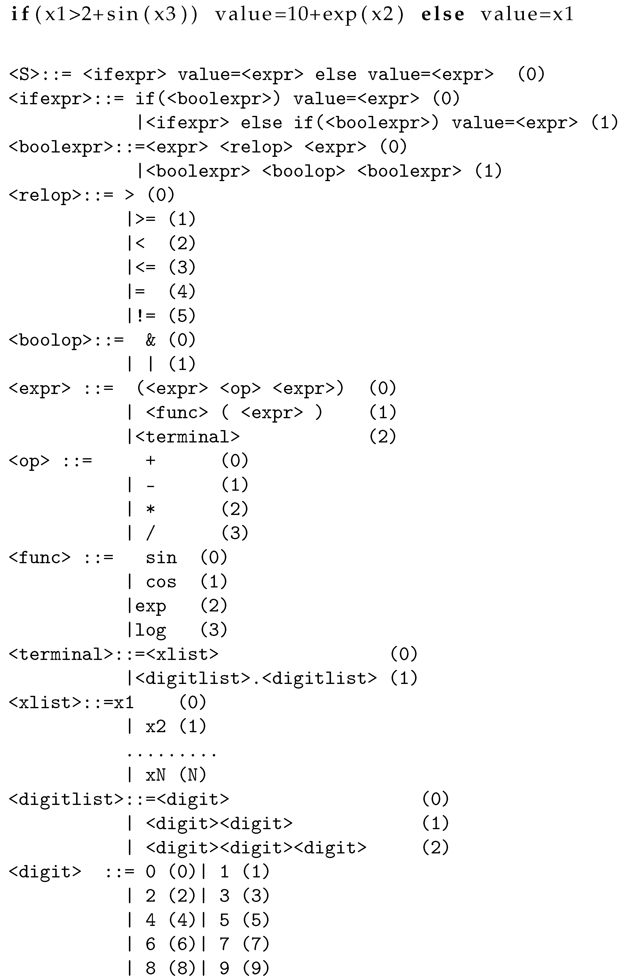
Figure 2.
Example of one-point crossover.
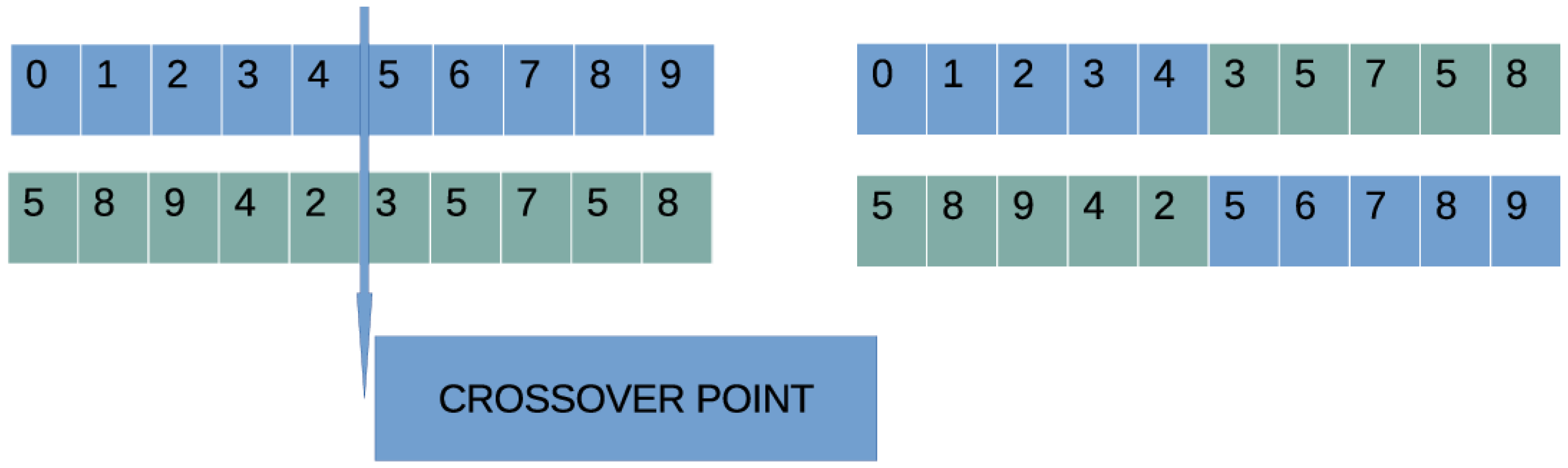
Figure 3.
Comparison of average classification error for RBF and artificial neural network for different number of weights.
Figure 3.
Comparison of average classification error for RBF and artificial neural network for different number of weights.
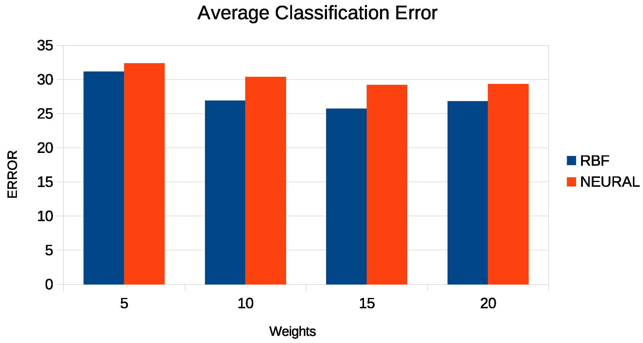
Figure 4.
Example of constructed program for the wine dataset.

Figure 5.
Example program for the housing dataset.


Table 1.
Experimental parameters.
| PARAMETER | VALUE |
|---|---|
| 500 | |
| 2000 | |
| 0.1 | |
| 0.5 |
Table 2.
Experiemental results for classification datasets.
| DATASET | RBF | MLP | SGD | LEVE | PROPOSED |
|---|---|---|---|---|---|
| AUSTRALIAN | 34.89% | 32.21% | 42.92% | 22.17% | 14.84% |
| BALANCE | 33.42% | 8.97% | 6.16% | 14.10% | 10.40% |
| DERMATOLOGY | 62.34% | 30.58% | 45.52% | 50.98% | 29.40% |
| GLASS | 50.16% | 60.25% | 51.41% | 61.68% | 55.19% |
| HAYES ROTH | 64.36% | 56.18% | 60.23% | 57.97% | 32.08% |
| HEART | 31.20% | 28.34% | 43.57% | 27.57% | 19.70% |
| HEARTATTACK | 32.83% | 31.54% | 36.48% | 21.20% | 22.07% |
| HOUSEVOTES | 5.99% | 6.62% | 3.48% | 8.64% | 3.00% |
| IONOSPHERE | 16.22% | 15.14% | 10.14% | 13.10% | 11.11% |
| LIVERDISORDER | 30.84% | 31.11% | 33.69% | 29.40% | 32.32% |
| MAMMOGRAPHIC | 21.38% | 19.88% | 21.01% | 17.08% | 17.54% |
| PARKINSONS | 17.41% | 18.05% | 32.91% | 18.67% | 13.11% |
| PIMA | 25.75% | 32.19% | 35.32% | 24.53% | 24.90% |
| POPFAILURES | 7.04% | 5.94% | 3.43% | 5.24% | 5.33% |
| REGIONS2 | 37.49% | 29.39% | 41.29% | 37.77% | 26.87% |
| SAHEART | 32.19% | 34.86% | 34.70% | 29.78% | 30.97% |
| SONAR | 27.85% | 26.97% | 19.60% | 27.20% | 28.38% |
| STUDENT | 5.74% | 7.23% | 3.43% | 5.21% | 5.47% |
| WDBC | 7.27% | 8.56% | 17.95% | 7.98% | 5.66% |
| WINE | 31.41% | 19.20% | 29.08% | 34.69% | 11.35% |
| Z_F_S | 13.16% | 10.73% | 28.58% | 14.32% | 7.97% |
| ZO_NF_S | 9.02% | 8.41% | 29.00% | 9.73% | 8.20% |
| ZONF_S | 4.03% | 2.60% | 18.45% | 3.59% | 1.98% |
| Z_O_N_F_S | 48.71% | 65.45% | 60.09% | 61.04% | 45.98% |
| ZOO | 21.77% | 16.67% | 5.00% | 45.70% | 9.70% |
| AVERAGE | 26.90% | 24.28% | 28.54% | 25.97% | 18.94% |
Table 3.
Experiments for regression datasets.
| DATASET | RBF | MLP | SGD | LEVE | PROPOSED |
|---|---|---|---|---|---|
| ABALONE | 7.32 | 7.17 | 4.55 | 4.94 | 5.05 |
| AIRFOIL | 0.05 | 0.003 | 0.004 | 0.002 | 0.002 |
| BASEBALL | 78.89 | 103.60 | 146.46 | 112.75 | 51.18 |
| BK | 0.02 | 0.03 | 0.02 | 0.02 | 0.02 |
| BL | 0.01 | 5.74 | 0.002 | 0.09 | 0.01 |
| CONCRETE | 0.01 | 0.01 | 0.005 | 0.005 | 0.009 |
| DEE | 0.17 | 1.01 | 0.93 | 0.65 | 0.24 |
| DIABETES | 0.49 | 19.86 | 0.38 | 2.72 | 0.67 |
| HOUSING | 57.68 | 43.26 | 81.45 | 89.44 | 23.35 |
| FA | 0.01 | 1.95 | 0.02 | 0.02 | 0.01 |
| MB | 1.91 | 3.39 | 0.06 | 0.06 | 0.06 |
| MORTGAGE | 1.45 | 2.41 | 10.10 | 8.64 | 0.09 |
| NT | 8.15 | 0.05 | 0.01 | 0.06 | 0.08 |
| PY | 0.02 | 0.10 | 0.02 | 0.06 | 0.02 |
| QUAKE | 0.07 | 0.04 | 0.04 | 0.04 | 0.04 |
| TREASURY | 2.02 | 2.93 | 11.60 | 10.35 | 0.10 |
| WANKARA | 0.001 | 0.012 | 0.0002 | 0.0002 | 0.0004 |
| AVERAGE | 9.31 | 11.27 | 15.04 | 13.52 | 4.76 |
Table 4.
Experiments with the number of generations for the classification datasets.
| DATASET | |||
|---|---|---|---|
| AUSTRALIAN | 14.77% | 14.89% | 14.84% |
| BALANCE | 20.14% | 15.47% | 10.40% |
| DERMATOLOGY | 39.46% | 35.06% | 29.40% |
| GLASS | 57.10% | 55.38% | 55.19% |
| HAYES ROTH | 32.23% | 30.92% | 32.08% |
| HEART | 19.30% | 19.33% | 19.70% |
| HEARTATTACK | 23.80% | 22.57% | 22.07% |
| HOUSEVOTES | 4.13% | 4.17% | 3.00% |
| IONOSPHERE | 12.83% | 11.68% | 11.11% |
| LIVERDISORDER | 34.06% | 33.59% | 32.32% |
| MAMMOGRAPHIC | 17.95% | 17.81% | 17.54% |
| PARKINSONS | 13.63% | 14.00% | 13.11% |
| PIMA | 26.64% | 25.84% | 24.90% |
| POPFAILURES | 5.98% | 5.54% | 5.33% |
| REGIONS2 | 29.47% | 28.84% | 26.87% |
| SAHEART | 29.50% | 29.59% | 30.97% |
| SONAR | 26.95% | 26.45% | 28.38% |
| STUDENT | 6.15% | 5.80% | 5.47% |
| WDBC | 6.27% | 5.97% | 5.66% |
| WINE | 14.94% | 13.06% | 11.35% |
| Z_F_S | 9.80% | 8.87% | 7.97% |
| ZO_NF_S | 10.88% | 9.82% | 8.20% |
| ZONF_S | 2.46% | 2.58% | 1.98% |
| Z_O_N_F_S | 50.14% | 48.02% | 45.98% |
| ZOO | 14.90% | 11.70% | 9.70% |
| AVERAGE | 20.94% | 19.88% | 18.94% |
Table 5.
Experiments with the number of generations using the proposed method for the regression datasets.
Table 5.
Experiments with the number of generations using the proposed method for the regression datasets.
| DATASET | |||
|---|---|---|---|
| ABALONE | 5.42 | 5.30 | 5.05 |
| AIRFOIL | 0.003 | 0.002 | 0.002 |
| BASEBALL | 52.81 | 51.67 | 51.18 |
| BK | 0.02 | 0.02 | 0.02 |
| BL | 0.02 | 0.02 | 0.01 |
| CONCRETE | 0.01 | 0.01 | 0.009 |
| DEE | 0.30 | 0.27 | 0.24 |
| DIABETES | 0.45 | 0.46 | 0.67 |
| HOUSING | 25.51 | 23.97 | 23.35 |
| FA | 0.01 | 0.03 | 0.01 |
| MB | 0.05 | 0.05 | 0.06 |
| MORTGAGE | 0.13 | 0.11 | 0.09 |
| NT | 0.01 | 0.01 | 0.08 |
| PY | 0.02 | 0.02 | 0.02 |
| QUAKE | 0.04 | 0.04 | 0.04 |
| TREASURY | 0.12 | 0.11 | 0.10 |
| WANKARA | 0.0004 | 0.0004 | 0.0004 |
| AVERAGE | 4.99 | 4.83 | 4.76 |
Publisher’s Note: MDPI stays neutral with regard to jurisdictional claims in published maps and institutional affiliations. |
© 2022 by the author. Licensee MDPI, Basel, Switzerland. This article is an open access article distributed under the terms and conditions of the Creative Commons Attribution (CC BY) license (https://creativecommons.org/licenses/by/4.0/).
Share and Cite
MDPI and ACS Style
Tsoulos, I.G. Learning Functions and Classes Using Rules. AI 2022, 3, 751-763. https://doi.org/10.3390/ai3030044
AMA Style
Tsoulos IG. Learning Functions and Classes Using Rules. AI. 2022; 3(3):751-763. https://doi.org/10.3390/ai3030044
Chicago/Turabian StyleTsoulos, Ioannis G. 2022. "Learning Functions and Classes Using Rules" AI 3, no. 3: 751-763. https://doi.org/10.3390/ai3030044
APA StyleTsoulos, I. G. (2022). Learning Functions and Classes Using Rules. AI, 3(3), 751-763. https://doi.org/10.3390/ai3030044