Vision Based Drone Obstacle Avoidance by Deep Reinforcement Learning

Abstract

Research on autonomous obstacle avoidance of drones has recently received widespread attention from researchers. Among them, an increasing number of researchers are using machine learning to train drones. These studies typically adopt supervised learning or reinforcement learning to train the networks. Supervised learning has a disadvantage in that it takes a significant amount of time to build the datasets, because it is difficult to cover the complex and changeable drone flight environment in a single dataset. Reinforcement learning can overcome this problem by using drones to learn data in the environment. However, the current research results based on reinforcement learning are mainly focused on discrete action spaces. In this way, the movement of drones lacks precision and has somewhat unnatural flying behavior. This study aims to use the soft-actor-critic algorithm to train a drone to perform autonomous obstacle avoidance in continuous action space using only the image data. The algorithm is trained and tested in a simulation environment built by Airsim. The results show that our algorithm enables the UAV to avoid obstacles in the training environment only by inputting the depth map. Moreover, it also has a higher obstacle avoidance rate in the reconfigured environment without retraining.

1. Introduction

Also known as unmanned aerial vehicle (UAV), the drone refers to a flying object without a human pilot aboard. Currently, UAVs mainly rely on remote control in practical applications. The maintenance cost is high, the response speed is slow, and it is subject to the transmission quality of the communication channel. Therefore, autonomous motion planning is urgently required in the UAV sector. One of the major requirements for the motion planning of drones is obstacle avoidance. Compared to ultrasonic and laser radar technology, the visual obstacle avoidance technology is more suitable for UAVs, because visual sensor does not require a transmitting device. In addition, the receiving device is simple, making it easier for UAVs to achieve small size, light weight, and low energy consumption. Visual obstacle avoidance technology also does not require signal transmission. This means that there is no radiation and signal interference. Furthermore, it is not limited by geographical conditions and locations.

In the visual obstacle avoidance strategy, visual simultaneous localization and mapping (VSLAM) is one of the main representative methods applied to land robots [1].

The goal of SLAM is to construct a real-time map of the surrounding environment based on sensor data and infer its own location based on this map [2]. A SLAM that uses only a camera as an external sensor is called visual SLAM (VSLAM [3]). Compared to the traditional SLAM algorithm, it has the advantages of rich visual information and low hardware cost. Owing to the complexity of the flight environment, VSLAM has no significant effect on drones. Although the SLAM solution that simultaneously uses cameras, lidar, and other sensors at the same time can achieve better results [4], it also has some limitations, such as high dependence on the computing performance of the processing chip, and difficulty in coping with visual changes in the target area.

With the development of machine learning, many obstacle avoidance solutions based on deep learning have emerged. Such methods are mainly divided into supervised and unsupervised learning and deep reinforcement learning. In supervised learning, a large amount of data must be collected in the training environment of the drone before training. This method is only feasible if the dataset is sufficiently large and has high-quality labels. Considering the complexity of the drone operating environment, it is very difficult to manually create a dataset. Therefore, some studies have used unsupervised learning methods to label datasets automatically. In the field of UAVs, research related to unsupervised learning mainly tends to assist the model of supervised learning to automate the production of datasets to reduce the human effort of labeling data [5]. On the other hand, the deep reinforcement learning (DRL) method can solve the problem of creating a dataset by making the drones collect data by themselves in the training environment.

In contrast to the discrete action space obstacle avoidance strategy [6] that has achieved certain results in recent years, in this research we use the soft actor critic algorithm (SAC) [7,8] to implement the UAV obstacle avoidance scheme based on continuous action space, so that the UAV can make more accurate and smooth action selection. We use the depth maps as input and combine SAC with a variational auto-encoder (VAE) to train the UAV to complete obstacle avoidance tasks in a simulation environment composed of multiple wall obstacles.

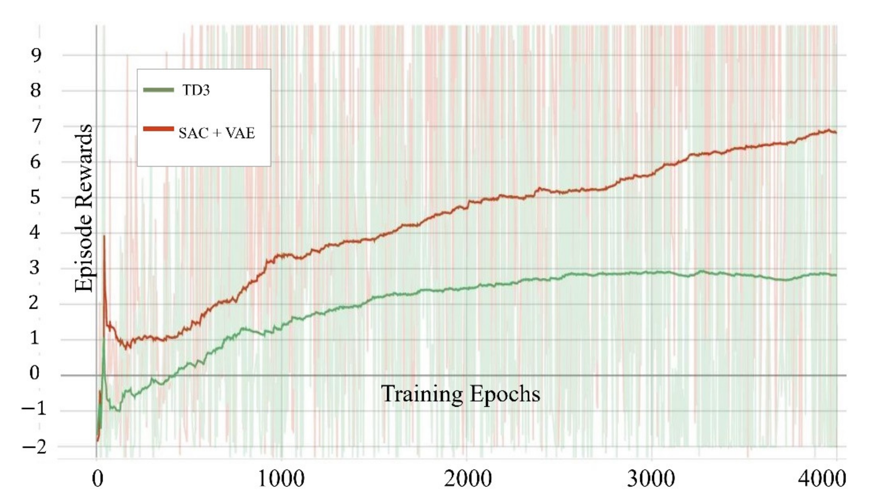
Experiments have proved that by using the delay-learning method, our algorithm can obtain a more stable training effect in the UAV obstacle avoidance task than the general SAC algorithm. Compared with the traditional DRL algorithm that directly uses images as input in UAV obstacle avoidance tasks, our model combining VAE and SAC can converge faster and achieve higher rewards in UAV obstacle avoidance tasks.

In this study, Airsim is used as the simulator, Unreal Engine 4 as the image engine, and python pytorch as the machine learning framework. The three constitute an integrated machine learning simulation environment. In the simulation environment, the quadrotor aircraft acts as the learning agent. The front depth image of the environment collected by Airsim from the UE4 engine serves as the input data. The output is the flying and obstacle avoidance action taken by the agent in each time step.

The results show that the trained agent can not only achieve an average obstacle avoidance rate of 90% in the training environment, but also has an average obstacle avoidance rate of over 80% and over 70% in an environment where obstacles are rearranged and reconstructed. This means that our model has not only a good obstacle avoidance ability in the training environment, but also a certain ability to adapt to the new environment.

The rest of this paper is organized as follows: Section 2 describes related works on the visual based and deep reinforcement learning strategy of drone navigation. Section 3 focuses on the methods used in this research. Section 4 explains the experimental process of the study in detail. Finally, Section 5 summarizes our research results along with their limitations and proposes future research plans.

2. Related Work

Recently, several drone algorithms based on deep learning have emerged, and they have been applied to various drone-related tasks, such as localization and navigation [9]. Among them, supervised learning has many research results on drone control, while the main results of unsupervised learning are still concentrated on feature extraction tasks such as action recognition. Deep reinforcement learning has also made certain breakthroughs in the field of drone control, and it is increasingly becoming mainstream.

2.1. UAV Navigation Based on Supervised Learning

Supervised learning requires a large amount of data as the basis for training. With the gradual enrichment of datasets, supervised learning can also empower UAVs to complete more complex tasks. With different datasets, the tasks that drones can accomplish under supervised learning are also different. For example, using convolutional neural networks, UAVs can be trained to navigate autonomously and find a specific target in small indoor environments using only monocular vision [10]. By collecting collision and crash data, drones can be trained to effectively avoid collisions [11]. In contrast, by using a dataset of gates captured in various environments, drones can be trained to pass through the gate in a targeted manner [12]. Similarly, by collecting a large amount of data on urban roads, drones can also navigate in urban environments and avoid common urban obstacles [13]. Because UAV navigation technology that uses supervised learning can solve problems in various scenarios in a targeted manner, it already has some mature applications in actual industrial technologies, such as the Internet of Things (loT) systems [14]. Collectively, these studies outline a critical role for datasets in UAV navigation with supervised learning. However, supervised learning via datasets has two major drawbacks: (1) Researchers need to manually collect and label a large amount of data; (2) the data are highly oriented to a specific environment, so the model needs to be retrained or an entirely new model needs to be rebuilt when transferred to a new environment.

2.2. The Auxiliary Role of Unsupervised Learning for Drone Navigation

Although unsupervised learning cannot complete the drone navigation task independently, it has a certain auxiliary effect on supervised learning and reinforcement learning models. In addition to helping supervised learning to label data [15], unsupervised learning models can also estimate depth maps from monocular vision images [5,16]. There are also examples of using unsupervised learning to train rescue drones for human detection [17]. In this study, we use VAE [18] to process visual perception information, which is also a method of using unsupervised learning to assist DRL training.

2.3. UAV Navigation Based on Reinforcement Learning

Reinforcement learning adopts the “trial and error” mechanism in human and animal learning. It emphasizes learning in interaction with the environment and uses evaluative feedback signals to optimize decision-making. Because reinforcement learning does not need to be given teacher signals in various states during the learning process, it has broad application prospects in solving complex optimization decision-making problems, such as UAV navigation.

Reinforcement learning can be divided into value function-based reinforcement learning and policy-based reinforcement learning. In reinforcement learning based on the value function, Q learning algorithm is the most commonly used learning algorithm. Several studies have applied it to the navigation of mobile robots [19,20]. However, because the state space and action space of the Q-learning algorithm are both discrete, the planned route has poor flying ability and finds it difficult to deal with dynamic threats. In response to these shortcomings, researchers have proposed a combination of deep learning and reinforcement learning to form a deep reinforcement learning (DRL) algorithm to meet the needs of state space or action space continuity. The initial DRL was Deep Q Network (DQN), proposed by DeepMind in 2013 [21]. Some studies [22,23] introduced different improved DQNs in path planning and achieved satisfactory results. However, since the action space of the DQN is still in discrete form, there is still room for further improvement in the quality of the planned path.

To achieve a continuous state space and action space, researchers further combined another branch of reinforcement learning with deep learning: policy-based reinforcement learning and proposed a policy-based DRL algorithm, including the deep deterministic policy gradient algorithm (deep deterministic policy gradient, DDPG) [24] and distributed proximal policy optimization (DPPO) [25].

2.4. Visual Perception

Although some studies have attempted to apply policy-based DRL algorithms to the path planning of UAVs and unmanned vehicles [26], the scenarios involved in these studies are still far from the complex operating environment of UAVs. In fact, the training of end-to-end vision-based DRL navigation strategy is very time-consuming, because the CNN used to learn vision-based functions involves multiple matrix operations. Moreover, CNN models require millions of images, and several days of training to acquire an adequate DRL policy [27,28]. In addition, because there are many constraints in a complex environment, compared with discrete space-based methods, such as Q learning and DQN, the policy-based DRL algorithm may not easily converge [29]. For policy-based DRL algorithms, obtaining feature-rich and compact visual perception information from images is a very important research direction.

In the field of UAV navigation, some studies tend to simplify the image to achieve the effect of compressing information and retaining features. For example, in [30], while training the actor-critic algorithm, a U-net is skillfully trained to convert the RGB image into a dense optical flow, and then the dense optical flow matrix is flattened as the state of DRL training.

VAE-based models are often used to extract low-dimensional feature information from images [18,31]. Microsoft recently used a framework called cross modal variational autoencoder (CM-VAE) to generate tightly bridged representations to simulate the reality gap [32]. The perception module of the system compresses the input image into the above-mentioned low-dimensional representation, from 27,648 variables to the most basic 10 variables that can describe it. These 10 variables that can be decoded into blurred images are used to replace the image itself for supervised learning and output the position information of the gate that the drone needs to pass through and the drone’s velocity. Using only the dataset processed by CM-VAE to train in a simulated environment can achieve the effect of completing the same task in a real environment. This makes it possible to use VAE for visual perception in the field of UAV DRL obstacle avoidance.

In this research, we attempt to combine VAE as an unsupervised learning auxiliary role with a policy-based DRL algorithm. We use VAE to compress image information, and then use the compressed image information as a state to participate in the training of the SAC algorithm. This method makes the network structure in the DRL algorithm more lightweight, so that the UAV visual obstacle avoidance algorithm can converge faster while utilizing less hardware resources. In the next section, we introduce the model composition and algorithm structure in detail.

3. Simulation Experiment Method

3.1. Simulation Environment

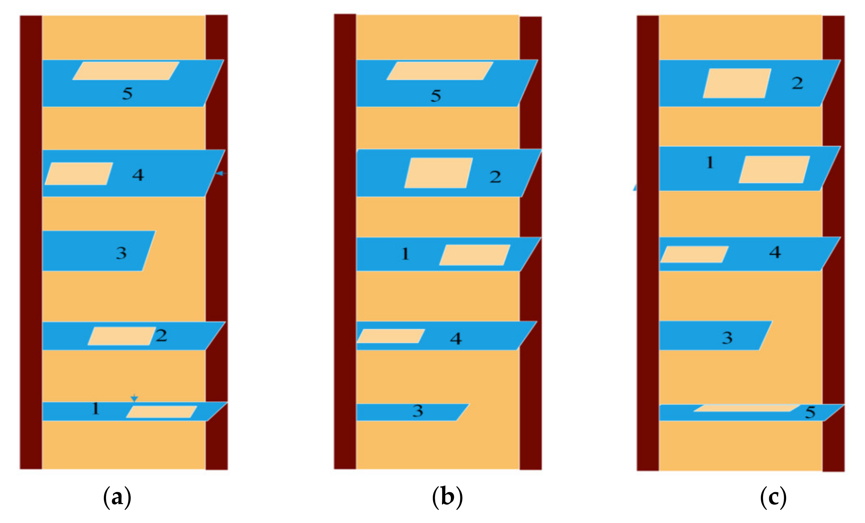
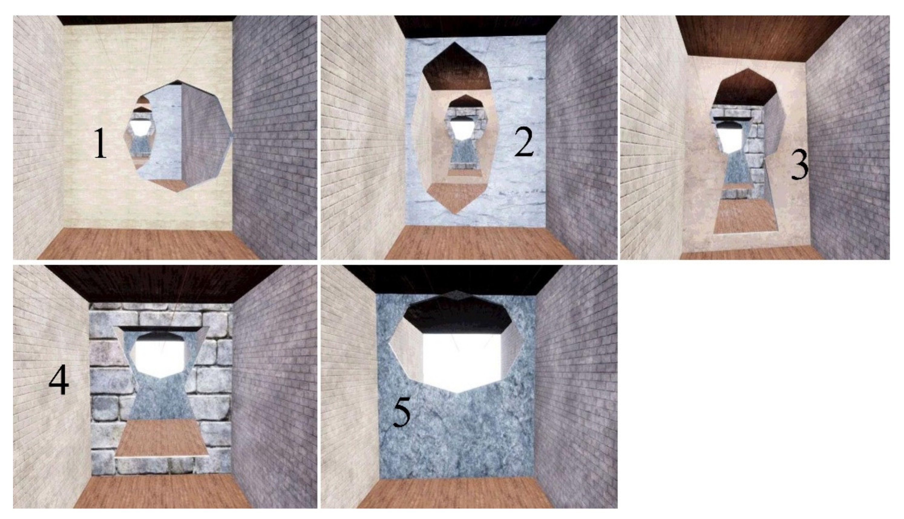
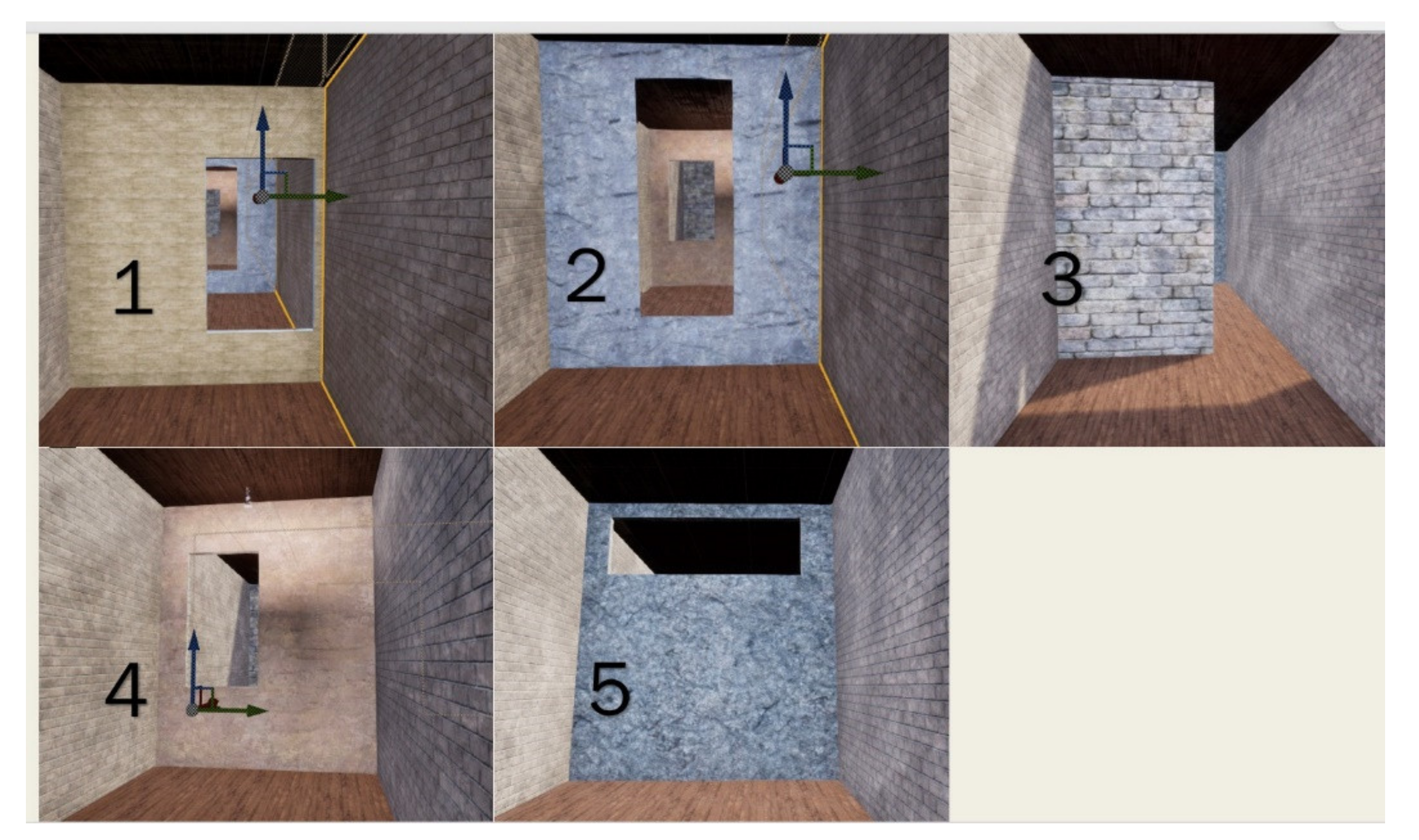
Airsim is an open-source drone and unmanned vehicle simulator launched by Microsoft [33]. It supports Unity 3D and Unreal 4 graphic engines. In this study, we chose Unreal 4, which has a variety of drawing tool libraries. Researchers can construct detailed scenes and obstacles with minimal effort. This study utilizes a rectangular closed corridor built by the Unreal Engine as the flying environment of the drone.

Binocular depth cameras can obtain high-resolution depth maps of immediate scenes. Owing to their small size and low power consumption, they are suitable for scene recognition when used with forward moving drones. In Airsim, we can directly retrieve the front depth map generated by the binocular depth camera. In the experiment, we used these depth maps as input to the deep reinforcement learning network.

3.2. Soft-Actor-Critic Framework

Among the DRL algorithms for continuous control, currently there are three mainstream algorithms. PPO [34] is an algorithm that requires a large amount of sampling to learn, and it is difficult to adapt it to the complex working environment of drones. DDPG is a deterministic strategy, that is, only the optimal action is considered in each state. When using DDPG, we found that it has a strong dependence on the parameters. The optimal solution depends on the tuning of a large number of parameters and repeated training. SAC cleverly combines the actor-critic algorithm with maximum-entropy reinforcement learning. Compared with DDPG, SAC is a random strategy that can explore a variety of optimal routes in complex environments.

For a general DL, the learning goal is straightforward, which is to learn a policy to maximize the accumulated reward expectation:

$${\mathsf{\pi }}^{*}=\arg \underset{\mathrm{x}}{\max }\mathrm{E}\left({\mathrm{s}}_{\mathrm{t}},{ \mathrm{a}}_{\mathrm{t}}\right) ~ {\mathsf{\rho }}_{\mathsf{\pi }}\left[{{\displaystyle \sum }}_{\mathrm{t}}\mathrm{R}\left({\mathrm{s}}_{\mathrm{t}},{ \mathrm{a}}_{\mathrm{t}}\right)\right]$$

(1)

In maximum entropy reinforcement learning, in addition to the above basic requirements, the entropy of each action output of each policy is required to be the maximum:

$${\mathsf{\pi }}^{*} =\arg \underset{\mathrm{x}}{\max }\mathrm{E}\left({\mathrm{s}}_{\mathrm{t}},{ \mathrm{a}}_{\mathrm{t}}\right) ~ {\mathsf{\rho }}_{\mathsf{\pi }}\left[{{\displaystyle \sum }}_{\mathrm{t}}\mathrm{R}\left({\mathrm{s}}_{\mathrm{t}},{ \mathrm{a}}_{\mathrm{t}}\right)+ \mathsf{\alpha }\mathrm{H}\left(\mathsf{\pi }\left(·|{\mathrm{s}}_{\mathrm{t}}\right)\right)\right]$$

(2)

Under such a strategy, the probability of each action output will be dispersed as much as possible, rather than concentrated on one action, such that the agent has stronger exploration ability and robustness.

In Equation (2), temperature α is the weight of entropy. Because of the constant change of reward, the use of a fixed temperature will make training unstable, so it is necessary to adjust this temperature automatically. Here, SAC constructs a constrained optimization problem, so that the average entropy weight is limited, but the entropy weight is variable in different states:

$$\underset{{\mathsf{\pi }}_0 :\mathrm{T}}{\max }{\mathrm{E}}_{{\mathsf{\rho }}_{\mathsf{\pi }}}\left[{{\displaystyle \sum }}_{\mathrm{t}=0}^{\mathrm{T}}\mathrm{R}\left({\mathrm{s}}_{\mathrm{t}},{ \mathrm{a}}_{\mathrm{t}}\right)\right]\mathrm{s}.\mathrm{t} \mathrm{E}\left({\mathrm{s}}_{\mathrm{t}},{ \mathrm{a}}_{\mathrm{t}}\right) ~{ \mathsf{\rho }}_{\mathsf{\pi }}\left[-\log \left({\mathsf{\pi }}_{\mathrm{t}}\left({\mathrm{a}}_{\mathrm{t}}{|\mathrm{s}}_{\mathrm{t}}\right)\right)\right]\ge \mathrm{H}\forall \mathrm{t}$$

(3)

By automatically adjusting the temperature, the agent can at first increase it when exploring a new area to explore more space. After becoming familiar with a given area, it gradually decreases the temperature to stabilize the strategy choice.

During the SAC training period, we use strategy and environment interaction and store the data of each interaction, the current state ${\mathrm{s}}_{\mathrm{t}}$, the behavior ${\mathrm{a}}_{\mathrm{t}}$, the reward ${\mathrm{r}}_{\mathrm{t}}$, and the post-action state ${\mathrm{s}}_{\mathrm{t}+1}$ into the buffer. After that, we sample (${\mathrm{s}}_{\mathrm{t}}$, ${\mathrm{s}}_{\mathrm{t}+1}$, ${\mathrm{r}}_{\mathrm{t}}$, ${\mathrm{a}}_{\mathrm{t}}$) from the buffer and estimate its quality (Q value) for the transition ${\mathrm{s}}_{\mathrm{t}}$→${\mathrm{a}}_{\mathrm{t}}\to {\mathrm{s}}_{\mathrm{t}+1}$. 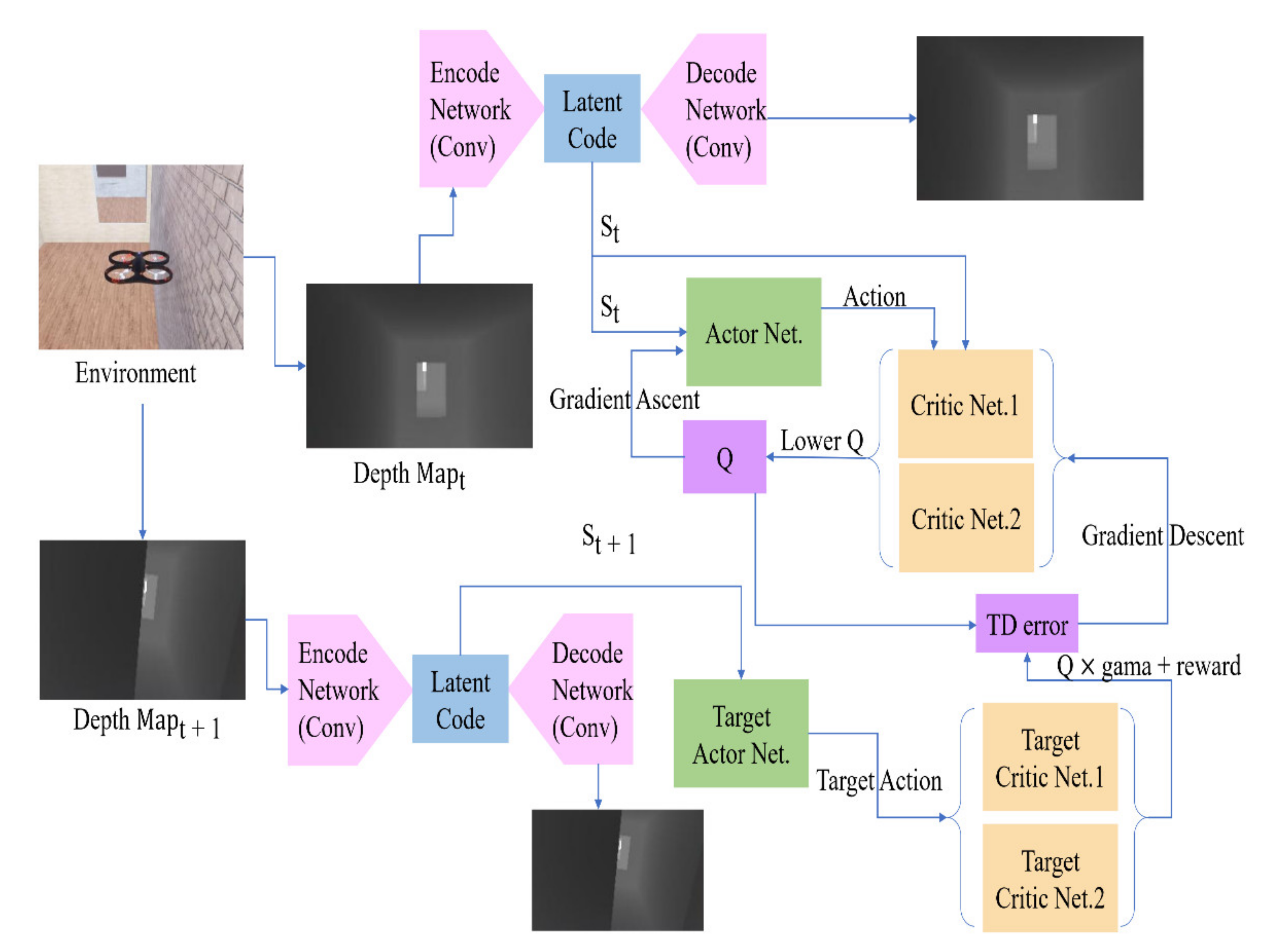We use this Q value to weigh our strategy and optimize the strategy in the direction of maximizing it. The workflow of the entire reinforcement learning system is illustrated in Figure 1. We simultaneously train a VAE to generate the same depth map as the input depth map. Then, we use VAE’s encode network to convert the depth map into latent code to participate in training as a state. Different from DDPG, SAC also uses two sets of critic networks to estimate the Q value. In our study, the smaller one is chosen as a candidate for updating.

Figure 1. Flow diagram of training of the whole system.

3.3. Variational Auto-Encoder

The policy-based DRL algorithm requires an algorithm to achieve high accuracy owing to the continuous action space, while DRL needs to use the newly trained model immediately after a few seconds of training. This means that this type of DRL can only use a relatively shallow network to ensure fast fitting. Moreover, the training data of reinforcement learning is not as stable as supervised learning, and it is not possible to divide the training and test sets to avoid overfitting. Therefore, such a DRL cannot be used in wide networks.

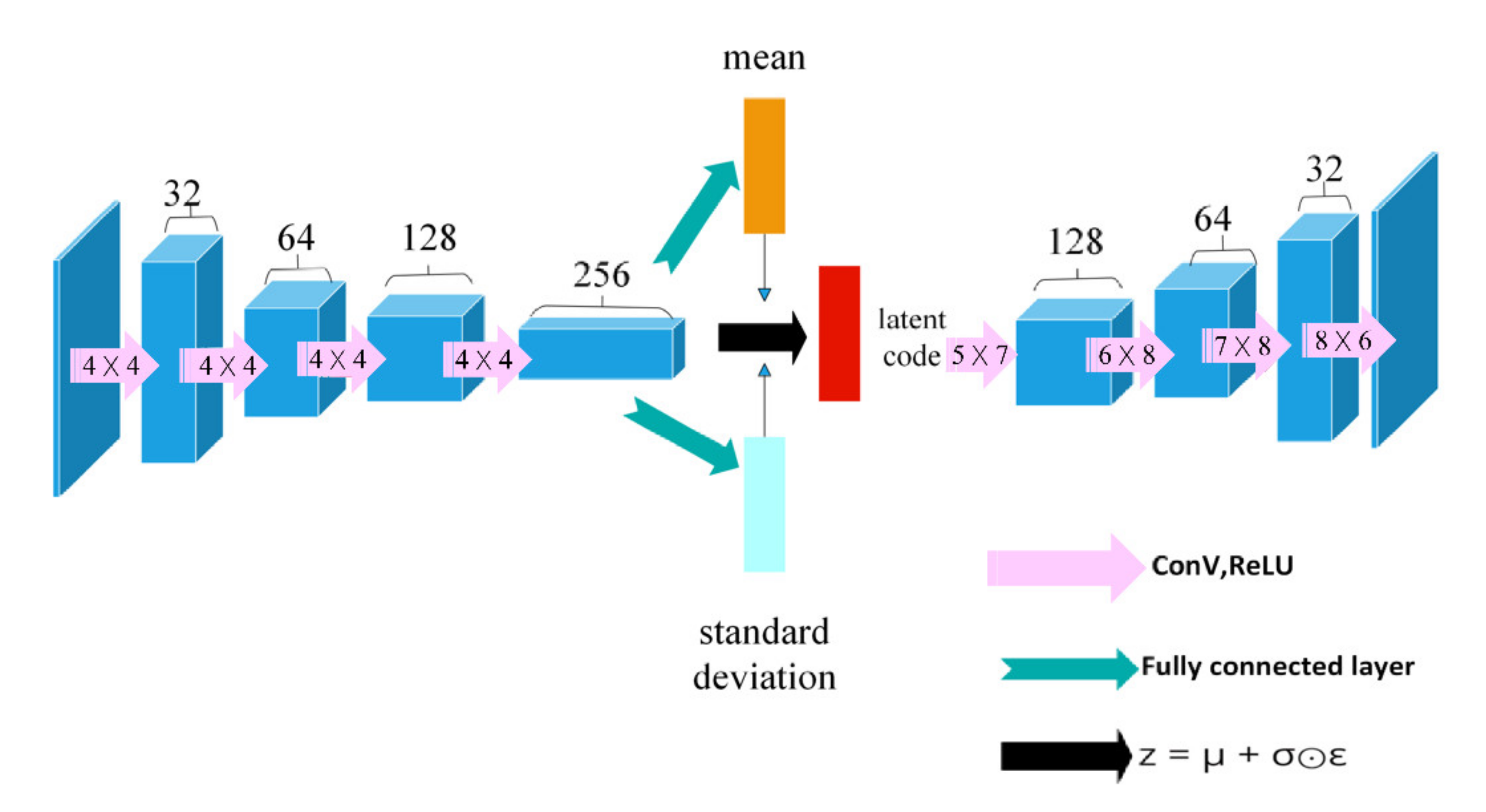
The policy-based DRL algorithm falls into a dilemma when faced with visual input. On the one hand, image recognition networks such as AlexNet [35] and ResNet [36] are too complicated for such algorithms, while on the other hand, using too lightweight networks is not sufficient to deal with complex image information. In order to solve this problem, we train a VAE synchronously during the first 10,000 steps of training. We let the same depth map be used as both the input of the VAE and the label map, so that the VAE can generate the depth map itself. When the VAE converges, the latent code generated in the VAE encode part is a code with a length of 32 and retains the original depth map features. Using such code as the state to participate in DRL training can make the state not only contain the effective information of the original image, but also light enough to use simple fully connected layers to achieve rapid convergence. The structure of the VAE we used is shown in Figure 2. The input depth map is a 128 × 72 grayscale image with a channel number of 1. The encode network is composed of a four-layer convolutional neural network, and each convolutional layer uses a (4 × 4) convolution kernel. Before decoding, we unflatten the latent code as data with a size of 1024 × 1 × 3. In order to successfully restore the data to its original size, we use convolution kernels with sizes (5 × 7), (6 × 8), (7 × 8), and (8 × 6) in the decode section.

Figure 2. The structure of the VAE.

3.4. The Structure of the Actor Network and the Critic Network

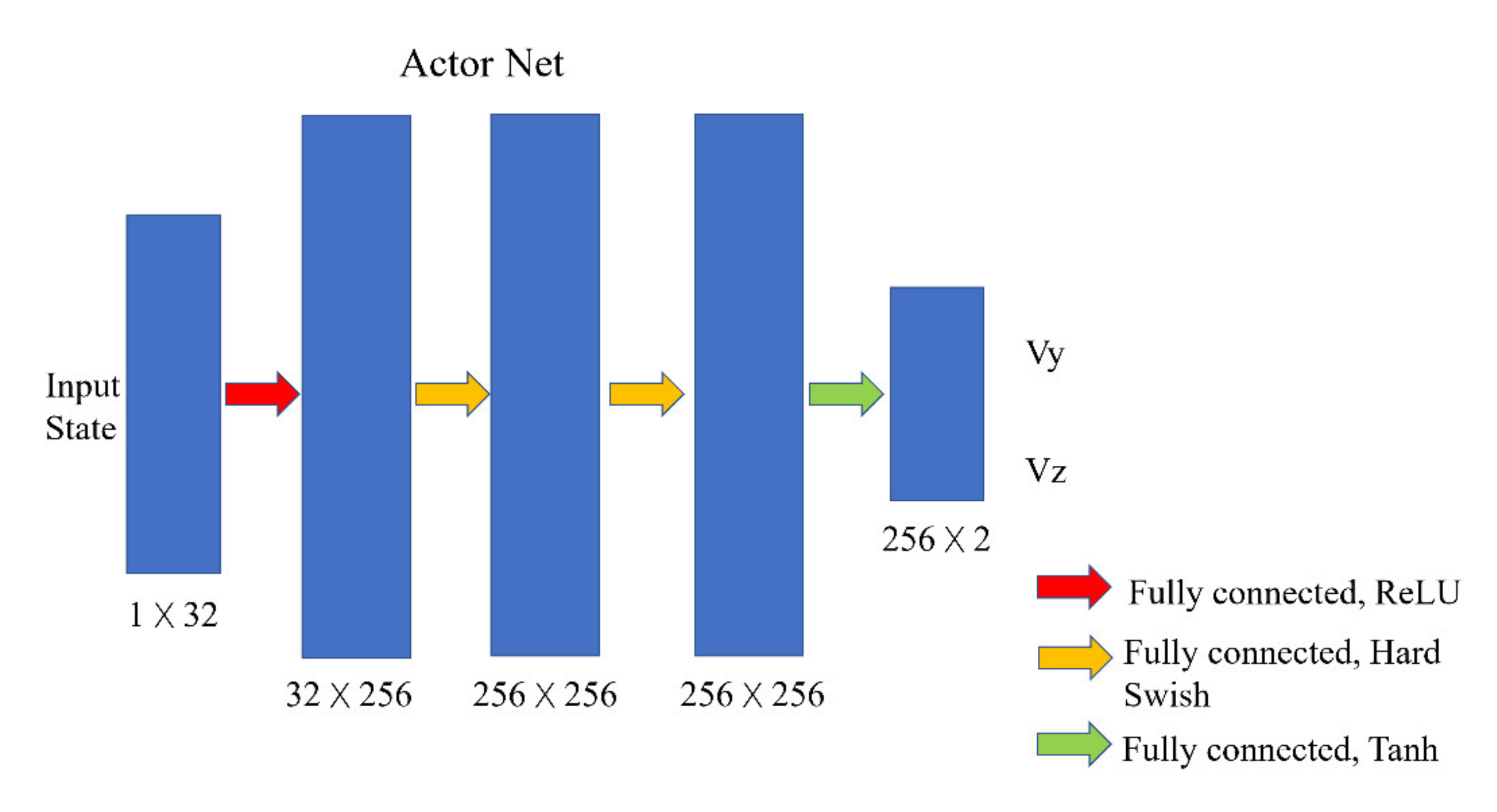
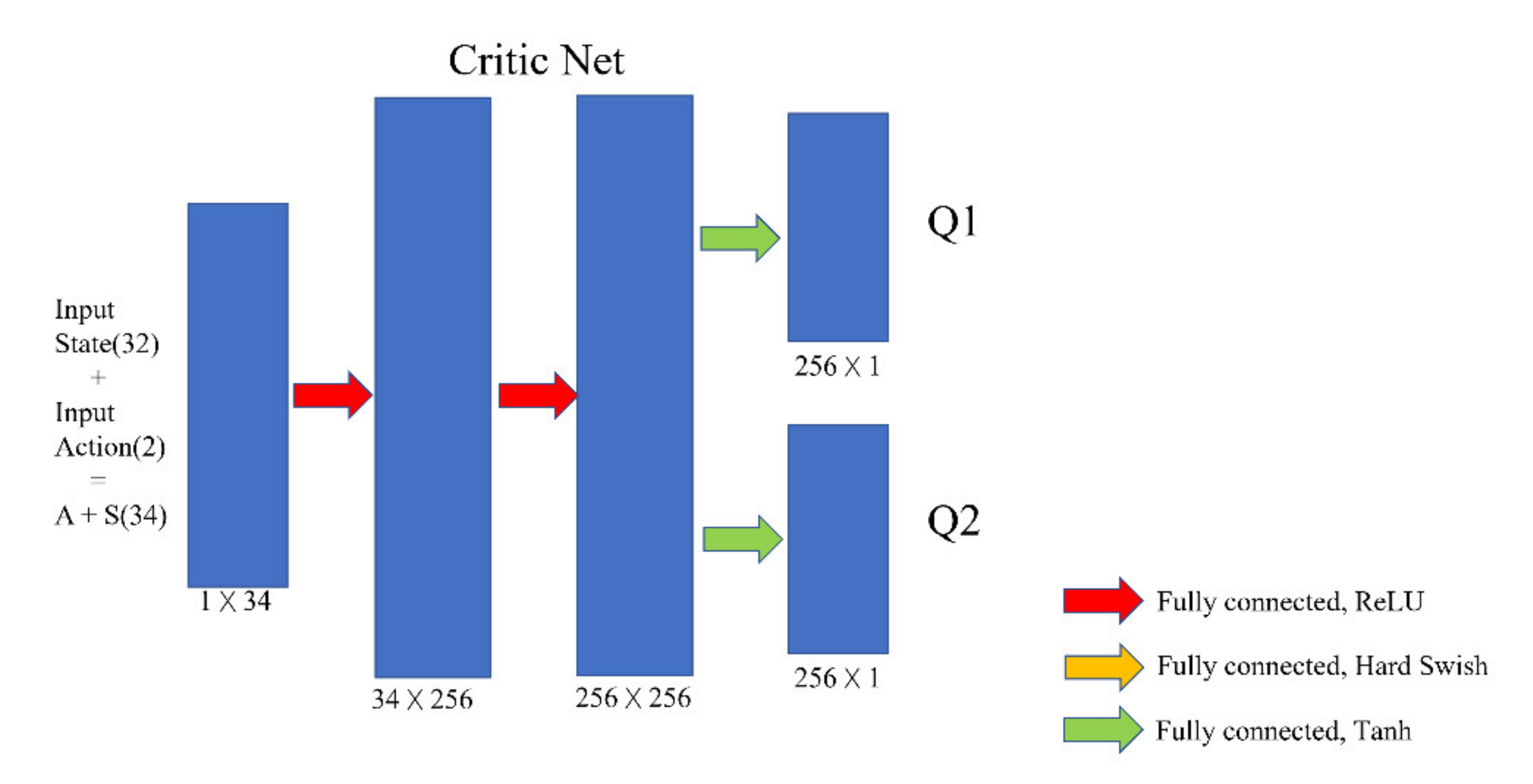
The structure of the actor and critic network is shown in the Figure 3. The actor network is a neural network composed of four fully connected layers. The 32-length latent code generated by the VAE is input into the actor network as the state. The output of the actor network has two values ranging from −1 to 1, representing the velocity of the drone in the y direction (left and right directions) and z direction (up and down directions).

Figure 3. Structure of the actor network and the critic network.

The critic network consists of three fully connected layers. Its function is to estimate the Q value that can be obtained when a certain action value is selected in a certain state. Therefore, the input value of the critic network is a combination of state and action, that is, a code with a length of 34. At the same time, to prevent the overestimation of the Q value, the SAC critic network uses two fully connected layers in the output layer to output two different Q values and take the smallest value in each update.

3.5. Replay Buffer

The size of the replay buffer is set to 2¹⁷, which means that 2¹⁷ number of actions, rewards, states, and next states are stored and sampled for training. However, unlike the replay buffer in traditional deep reinforcement learning, we divide the replay buffer into two parts:

(1)

Success buffer area that stores the success of avoiding obstacles; and

(2)

Regular buffer area for recording regular movements.

Dividing the replay buffer data into two categories is necessary because the data of normal flight and collision occupies a large proportion of the data collected by the drone, while the experience of avoiding obstacles only accounts for a small proportion. Especially at the very beginning of training, the UAV can hardly complete obstacle avoidance successfully. If all the data are stored in a single replay buffer and a certain amount of data are randomly extracted from it every time the model is updated, it will be difficult for the agent to learn successful experience.

Each time the model updates the learning networks, we extract data from the two buffers for training at a ratio of 0.125:0.875. Doing so ensures that a certain amount of successful experience can be learned every time the model is updated.

3.6. Reward Function

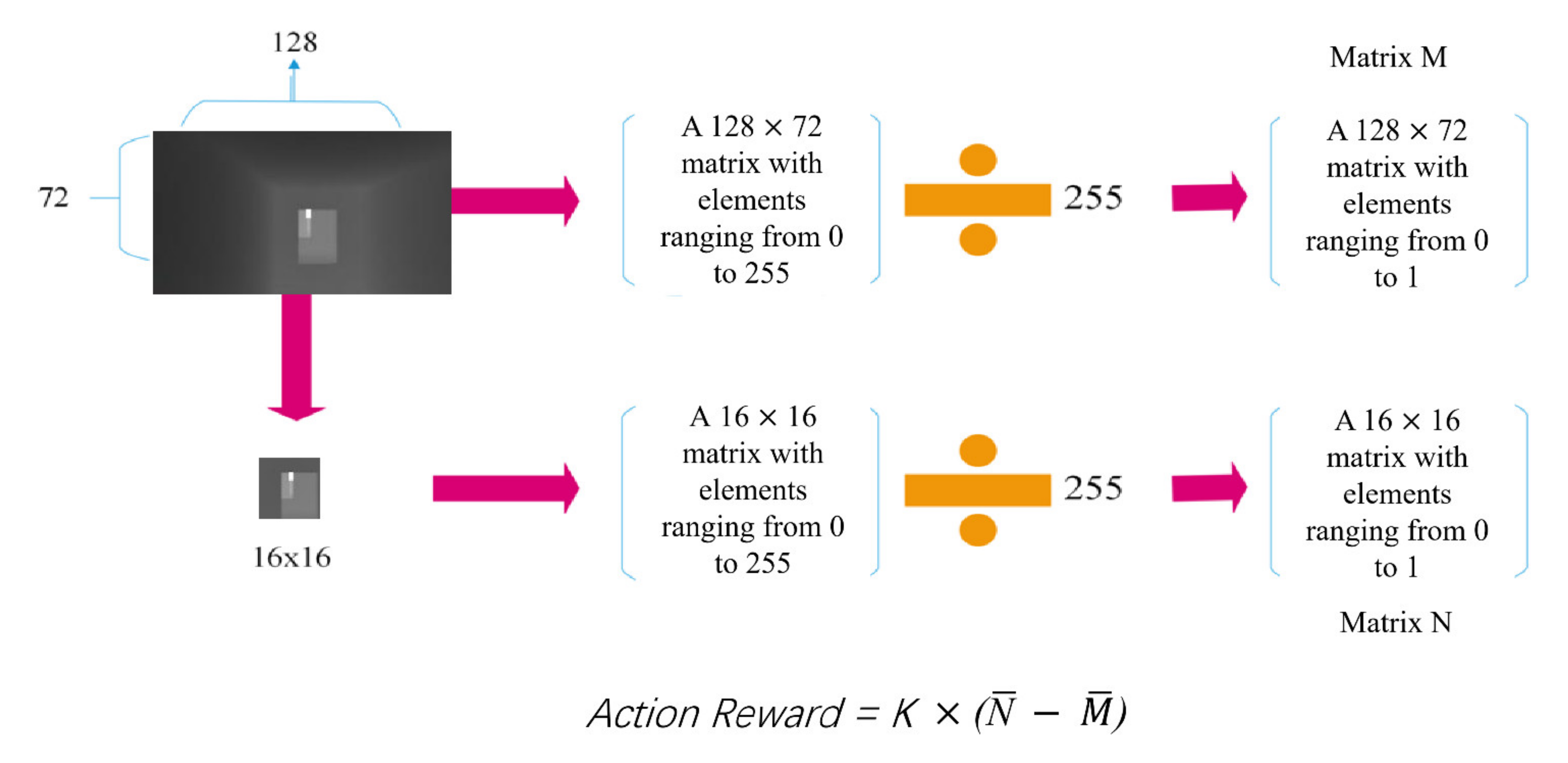
At the end of each step, the system gives the corresponding rewards or penalties based on whether it is a collision, whether it has been upgraded or whether it has reached the destination. Every time the drone moves, it records the center of the depth map ahead. The action reward takes the normalized average of the pixel values in the central 16 × 16 portion of the depth map matrix and subtracts normalized average value of the entire depth map matrix. The result will be multiplied by a parameter k. If the action reward is positive, it proves that the drone is moving away from the obstacle, that is, avoiding the obstacle, it is rewarded at this time. If the obstacle avoidance reward is negative, it means that the drone is approaching the obstacle and receives a certain penalty.

The specific reward values are presented in Table 1. The solution process of action reward is shown in the fourth row of Table 1 and Figure 4. The action reward is the difference between the normalized mean value of the central part of the depth map and the normalized mean value of the entire depth map.

Table 1. Reward function.

Reward Type	Reward Value
Collision	−2.0
Level Up	2.0
Reach Destination	2.0
Action Reward	Mean (depth map center (16 × 16)/255) − Mean (depth map/255)

Figure 4. The calculation process of action rewards.

3.7. Delay Learning

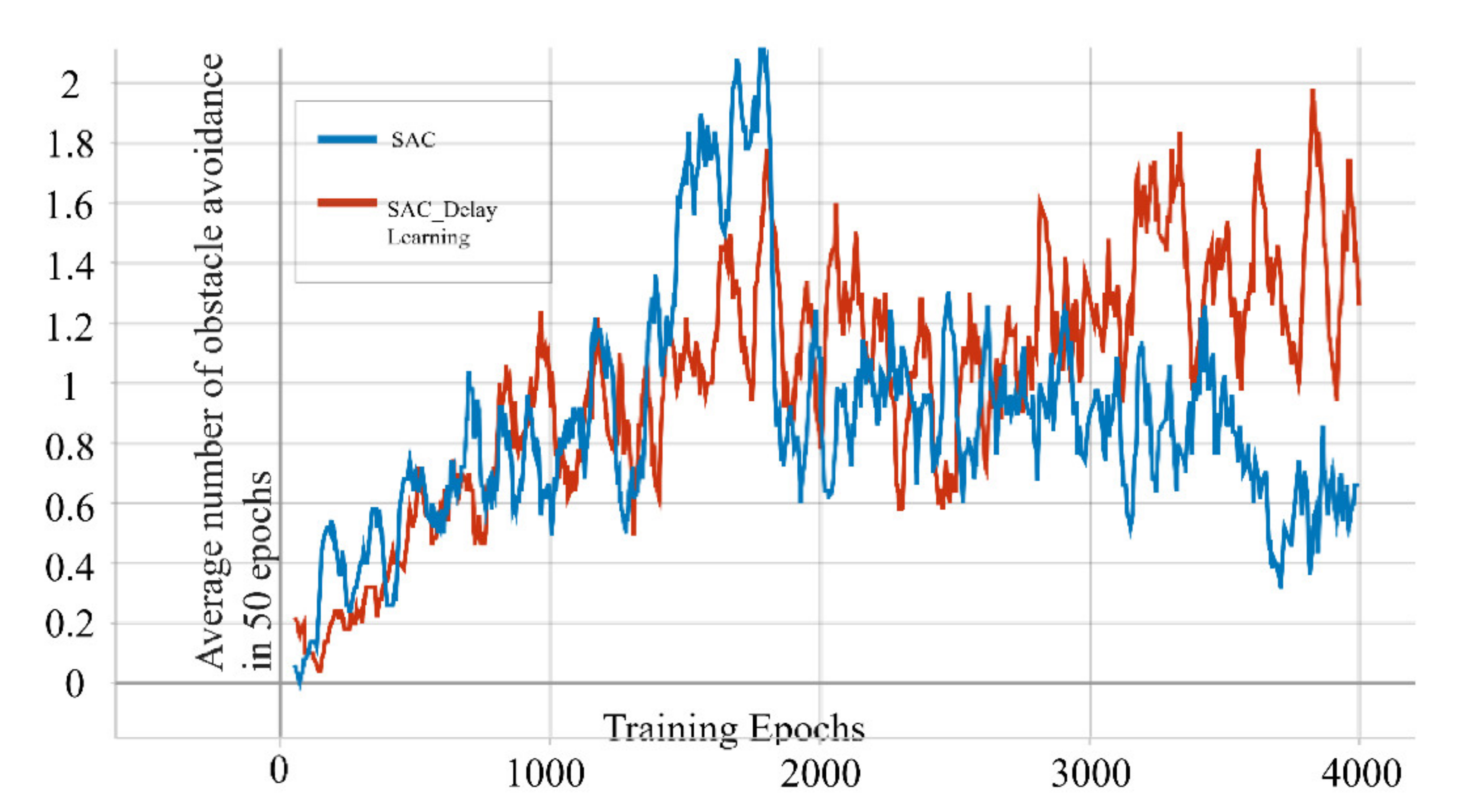
The original actor-critic type algorithm often uses a direct update scheme in the learning process, in which the critic and actor networks are updated at each time step. Theoretically, direct update will generate more training steps, thereby accelerating convergence. However, in practical applications, we found that this method frequently changes the policy selection plan during training, which confuses the agent about the strategy selection during learning and causes policy jittering.

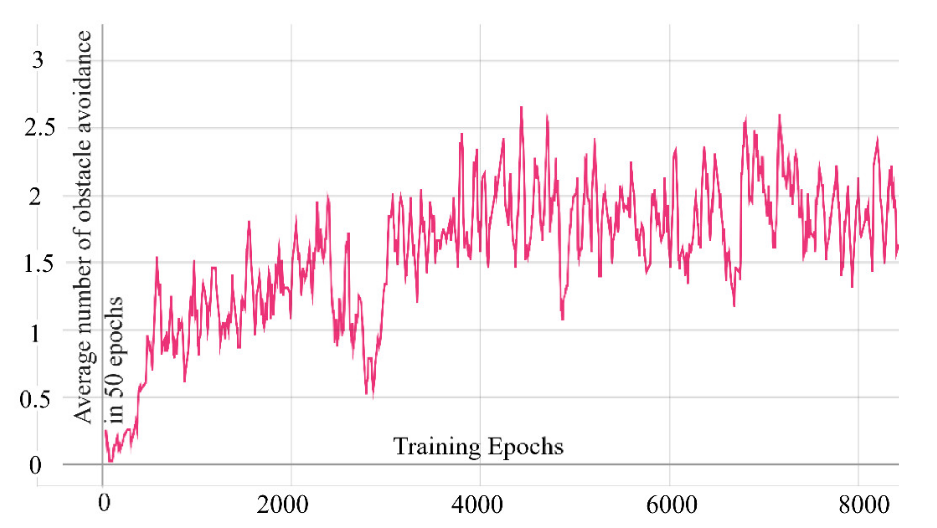
In order to solve this shortcoming, we designed a delayed learning scheme in which we delayed the update of the network until after the end of each epoch. This ensures that every complete flight of the drone follows the same policy. This method stabilizes the training process to a certain extent. To compare the differences between the two algorithms, we trained the two algorithms in the same environment for 4000 epochs and recorded their average obstacle avoidance times in the last 50 epochs. It can be seen from Figure 5 that although the difference in the results is not large, the conventional SAC has greater volatility in our task than the SAC with delayed learning.

Figure 5. SAC and delayed learning SAC are trained for 4000 epochs under our experimental task.

4. Experiments

4.1. Learning Environment

The settings of the workstation and simulation environment are listed in Table 2:

Table 2. Workstation and simulation environment settings.

Hardware/Frameworks	Parameters and Versions
CPU	AMD Ryzen Threadripper 3970 × 3.69 GHz
GPU	2 × NVIDIA RTX 3090
RAM	32 GB
Operating System	Windows 10
Program Language	Python 3.6
ML Library	Pytorch 1.9
CV Library	OpenCV 4.4
Simulator	Airsim 1.2.8
Game Engine	Unreal Engine 4.24.3

In this experiment, we used Unreal Engine to build a closed corridor with length 60 m, width 6 m, and height 7 m as the flying environment of the drone. Every ten meters in the corridor, a wall with different opening positions was used as an obstacle, as shown in Figure 6. We use these obstacles to divide the corridor into 5-level areas. Every time the drone crosses an obstacle in a single test, it is considered as a level-up. We consider the drone to take off from one end of the corridor and avoid all obstacles (passing through all the openings in the walls) as passing the test.

Figure 6. Five walls with different opening positions serve as obstacles in the experimental environment.

4.2. Training Process

The purpose of this experiment is to determine whether the soft-actor-critic network designed in Section 3 can train the UAV to attain obstacle avoidance capabilities. According to our reward function setting, the drone accumulates more rewards when it continuously avoids obstacles. These rewards will finally be settled as epoch rewards, that is, the rewards accumulated from take-off to crash or reach the end.

To enable the UAV to collect adequately diverse data during the training process, we used a segmented training method. After every 10 epochs, the drone takes off from the starting point of a new level. The switching of the starting point follows the order from level 1 to level 5 and returns to level 1 after training for 10 epochs in the level 5 environment.

4.3. Test Process

During the test, the drone takes off only at the initial starting point and attempts to avoid obstacles without any noise. The drone that passes the five obstacles safely and touches the end wall is deemed to have passed the test. To verify whether the drone can adapt to certain environmental changes, we repeatedly changed the order of the walls for testing, as shown in Figure 7. The test environment contained three different obstacles arranged sequentially. They are a training environment (the obstacle order is 12345) and two reconfigured environments (the obstacle order is 34125 and 53412).

Figure 7. The test environment. The test environment contained three different obstacles arranged sequentially. They are a training environment (a), the obstacle order is 12345 and two reconfigured environments (b,c), the obstacle order is 34125 and 53412.

After training, we tested the model with the highest average number of obstacle avoidances in the above three different environments. The drone flies 1000 epochs in these three environments under the control of the trained model. We recorded the number of successful avoidances of each obstacle and the average obstacle avoidance success rate after the tests.

To further verify the adaptability of the trained agent to the new environment, we constructed a test environment composed of five non-rectangular gates. In this test environment, the five obstacles are arranged in sequence according to the numbers shown in Figure 8, and the length, width, and height of the corridor are the same as those of the training environment.

Figure 8. Five non-rectangular obstacles in the new reconstructed test environment.

4.4. Results

In our experiments, the network was updated after each epoch. Figure 9 shows the graph with the training epochs on the horizontal axis and episode rewards on the vertical axis. It can be seen from Figure 9 that after about 200 epochs (only collecting data in the first 2000 steps without updating the network), episode rewards began to grow gradually. Since the use of reward to reflect the obstacle avoidance ability is not intuitive enough, we recorded the average number of obstacle avoidance times of the agent within 50 epochs during training. Fifty epochs were used to calculate the average value because the agent changed the starting point to the next level every 10 epochs. After 50 epochs, the starting point passed through all levels and then returned to level 1. In an ideal state, if the UAV completes all obstacle avoidance without any collision in 50 epochs, the average number of obstacle avoidances should be 3. As can be seen in Figure 10, as the training progresses, the average number of obstacle avoidances can gradually stabilize above 1 and approach 2 after 4000 epochs training.

Figure 9. The episode rewards graph.

Figure 10. The average obstacle avoidance times in 50 epochs.

We number the five obstacles from 1 to 5 in the order of the training environment. During the training progress, we save the model with the highest average number of obstacle avoidances. After completing the training, we test it in the training environment (the obstacles are arranged in the order of 12345), the two rearranged environments (the obstacles are in the order of 34125 and 53412, respectively), and a reconstructed environment (the shape of the obstacles is shown in Figure 8) for 100 epochs test. We record the number of times the drone reached each level in the three environments and calculate the obstacle avoidance rate of the drone using the following equation:

$$R=\frac{t_1 ÷100+ t_2 ÷100 + t_3 ÷100 + t_4 ÷100 + t_5 ÷100}{5}$$

(4)

where $R$ is the average obstacle avoidance rate, and $t_n$ is the number of times the nth obstacle has been avoided in 100 epochs. Refer to Table 3 for the specific data:

Table 3. Test results.

Obstacle Sequence	1 2 3 4 5	3 4 1 2 5	5 3 4 1 2	Environment Reconstructed
Level 1	96	90	85	72
Level 2	87	68	75	62
Level 3	74	56	60	44
Level 4	67	53	45	35
Level 5	59	46	33	24
Average obstacle avoidance rate	90.1%	85.9%	80.3%	75.4%

The experimental results show that as the number of training epochs increases, our model can finally achieve an obstacle avoidance rate of more than 90% in the training environment. After a long period of training, it can achieve an obstacle avoidance rate of over 80% in a rearranged environment and more than 70% in a reconstructed environment. This proves that when the training environment is sufficiently diverse, the model not only has the ability to learn quickly, but also has certain adaptability to the new environment.

At the same time, when comparing other similar research results horizontally, we can find that the UAV obstacle avoidance algorithm using TD3 needs 50,000 updates to reach more than 90% obstacle avoidance rate in the test environment when directly using the convolutional neural network as the policy network [37]. The actor critic algorithm that uses U-net for image data compact requires 2,000,000 updates to converge [22]. Our algorithm can achieve relatively ideal results in both the training environment and the reconfigured environment with only 8000 updates. This proves that our model can indeed solve the problem of slow convergence of the policy-based DRL algorithm on the UAV visual obstacle avoidance problem to a certain extent.

In order to compare the superiority of the model, we also conducted 4000 epochs training on our model and the TD3 algorithm in an experimental environment and compared the reward values obtained. As shown in Figure 11, the improved SAC in our experimental task is significantly better than the TD3 algorithm in both the growth rate and the peak value of the reward value.

Figure 11. The episode rewards graph of TD3 and SAC+VAE.

5. Conclusions

In this study, we proposed a deep reinforcement learning method using VAE to preprocess image data. This method enables UAVs to learn quickly and efficiently to avoid obstacles and does not need to rely on any sensors other than the depth camera. Compared to other visual obstacle avoidance algorithms, our method can complete obstacle avoidance in a continuous action space and does not require complex image recognition networks to perform DRL training.

However, this method still has room for improvement. We found that the trained VAE can indeed preserve the image features to a large extent while greatly simplifying the complex image information. In the next stage of research, we want to try to train VAE in a test environment to generate a depth map containing depth information or even a dense optical flow containing both depth and speed information from a given RGB image and test whether the latent code in this case as a state participating in DRL training has a good effect. If the RGB image can directly generate code that retains depth and even speed information, it means that the obstacle avoidance task of the UAV can be completed with a monocular camera, which makes the UAV lighter than the algorithm that requires a binocular camera.

SAC is a mature algorithm that does not rely on hyperparameters, but the quality of the reward function has a great impact on its learning efficiency. In the current experiment, in order to simplify the reward function, we fixed the advancement speed of the UAV to 1. This makes the UAV’s obstacle avoidance task in the simulation environment simpler than in the real world. The limitation of this method is that the drone cannot avoid obstacles that need forward speed adjustment or backward movement (reversing) to avoid collision. It will be our main task in the next stage of research to make a complete and accurate UAV obstacle avoidance in the full coordinate direction. In a completely reconstructed environment, the UAV’s obstacle avoidance capability shows some decline. Enhancing the ability of drones to adapt to the new environment will also be an important goal of our further research.