Research on Data-Driven Linear Prediction and Real-Time Control Method for Ship Rolling Control System in Beam Sea

Abstract

Predicting a ship’s motion trend in waves is crucial for safe navigation and operation. Existing prediction models are mostly based on the assumption of local linear dynamics, which can achieve great performance in idealized ocean environments. However, ships typically sail in real marine environments with regular or irregular waves, which makes the robustness and real-time performance of ship motion estimation models particularly important. To address this limitation, this paper proposes a global linear predictor (GLP) based on the Koopman operator, which can effectively represent the nonlinear rolling dynamics of ships. Furthermore, the GLP model is used to predict and control the rolling motion of a ship in real time. The proposed method is validated in both regular and irregular wave environments. The simulation experiment results show that the accuracy of the proposed method is about 14% higher than that of other classical methods on ships’ rolling dynamics. And it achieves a more than 91% rolling reduction efficiency in all wave conditions, significantly decreasing the amplitude of a ship’s rolling.

1. Introduction

Ships are subject to displacement and oscillatory motions induced by wind and waves in marine environments [1]. These motions generally involve six degrees of freedom (DOF) and are coupled with each other [2]. Among them, roll motion is particularly critical because of the geometric characteristics of ships and the associated risk of capsizing under severe wave conditions [3]. Therefore, ship roll motion has attracted considerable attention, and ship roll control has gradually developed into an important research field.

Various approaches have been developed to mitigate wave-induced rolling motion, including improving ship hydrodynamic properties and installing additional stabilization devices. For passive stabilization, ship designers can modify the submerged structure of the ship to increase roll damping. For example, bilge keels generate roll-damping moments through their interaction with water [4]. However, their stabilizing effectiveness is limited, making it difficult to significantly enhance ship stability under complex wave disturbances [5]. Consequently, a series of ship stabilization devices have been developed to suppress wave-induced roll motion [6], including rudders, fin stabilizers [7,8], anti-roll tanks, and gyrostabilizers. Rudders provide stabilizing moments through the coupling of roll and yaw [9]. Rudder-based studies usually rely on 4 DoF ship dynamics, including surge, sway, yaw, and roll [10], to achieve trajectory tracking and roll control simultaneously. However, the coupling among different degrees of freedom introduces strong nonlinearity [11], which imposes a high computational burden on the controller. By contrast, ship dynamics with dedicated roll stabilizers are commonly modeled as 1 DoF roll dynamics to simplify computation. Nevertheless, ship roll motion is inherently nonlinear [12]. In addition, roll hydrodynamic coefficients are difficult to obtain accurately through theoretical calculation, which further increases the difficulty of ship roll state prediction [13]. Especially under real sea conditions with irregular wave frequencies and amplitudes, prediction accuracy and computational delay caused by nonlinear dynamics become core challenges in ship roll control [14].

To address the state prediction and control problems of nonlinear ship roll dynamics, existing studies can be broadly divided into nonlinear control methods and linear-control-based methods. On the one hand, some studies have adopted nonlinear control algorithms to improve control accuracy in the presence of nonlinear dynamics [15]. For example, sliding mode control [6] has been proposed to compensate for nonlinear terms in ship roll dynamics by enforcing the system to operate near the sliding surface and thereby reduce control errors. However, sliding mode control may suffer from chattering, which can induce undesirable system vibrations. Cao et al. [16] designed a model predictive controller, which significantly improves control accuracy and mitigates the vibration problem. By explicitly modeling the nonlinear dynamics, these methods can improve state estimation and control accuracy. However, directly solving nonlinear optimization problems, which are typically nonconvex [17], increases computational delay and limits their applicability to real-time ship roll control [18].

On the other hand, classical linear controllers tend to exhibit better real-time performance than nonlinear controllers in practical applications. For example, Taskin et al. [19,20] proposed a controller based on $H_{\infty }$ control, and Song et al. [21] proposed an angular-rate-feedback controller for ship roll control. State prediction in these controllers typically relies on locally linearized roll models, which provide favorable real-time performance in both regular and irregular wave environments. However, local linear predictors are generally linearized around an equilibrium point, with higher-order terms neglected. Therefore, these approaches are generally most reliable under small-roll-angle assumptions, typically less than 30 degrees. Such local linear approximation may introduce prediction errors, especially under large-amplitude or irregular wave conditions, thereby degrading control accuracy.

Based on the above analysis, although local linear predictors can significantly improve real-time control performance, prediction errors caused by local linearization remain a key limitation. To overcome this limitation, this paper proposes a global linear predictor based on Koopman operator theory. The basic idea is to lift nonlinear dynamics into a high-dimensional space [22,23], in which the evolution of the lifted states can be approximated by a linear model [24]. Because the proposed predictor is identified from ship roll data, it can reduce dependence on analytically derived hydrodynamic coefficients [25] and improve prediction accuracy. Then, a model predictive controller (MPC) based on the proposed predictor is designed to control ship roll motion under diverse wave conditions. In this work, the stabilizing torque produced by the gyrostabilizer is utilized to counter wave disturbances, while the high-dimensional linear predictor and the MPC are used to estimate the system state and generate the control strategy, respectively. The main contributions of this paper are summarized as follows:

(1)

A data-driven global linear predictor based on Koopman operator theory is developed for nonlinear ship roll dynamics.

(2)

The proposed predictor is integrated with a linear MPC framework to achieve real-time ship roll control with a gyrostabilizer.

(3)

The prediction accuracy and roll reduction performance of the proposed method are validated under both regular and irregular wave conditions.

The paper is organized as follows. In Section 2.1, nonlinear ship roll dynamics with gyrostabilizers are described. In Section 2.2, the theory and realization of a global linear predictor based on the Koopman operator are presented in detail. In Section 2.3, a linear model predictive controller is designed for ship roll dynamics. In Section 3, numerical simulations are performed under several wave conditions to validate the effectiveness of the proposed algorithm. In Section 4, the strengths and limitations of the study are discussed. Finally, Section 5 presents the conclusions.

2. Materials and Methods

2.1. Dynamics of Ship’s Rolling with Gyrostabilizers

According to the principle of ship dynamics, a ship generates a 6 DOF motion in response to wave disturbances. However, since rolling motion is the most dominant factor causing ship instability, it is commonly simplified from a 6 DOF motion to a 1 DOF rolling motion, which has been used in many previous studies [14,21,26]. Therefore ship rolling dynamics are described as a second order nonlinear system:

$$I(\ddot{\varphi },t)+C(\dot{\varphi },t)+K(\varphi ,t)={\tau }_{wave}\left(t\right)$$

(1)

where $\varphi$, $\dot{\varphi }$, $\ddot{\varphi }$ indicate the ship’s rolling angle, angular velocity, and acceleration, respectively. $I(\ddot{\varphi },t)=(I_{xx}+J_{xx})\ddot{\varphi }$ is the mass moment of inertia, and $I_{xx}$, $J_{xx}$ are the ship’s rolling inertia and additional inertia, respectively. $C(\dot{\varphi },t)=c_1\dot{\varphi }+c_3{\dot{\varphi }}^3$ is the damping term, and $c_1$, $c_3$ are the 1st and 3rd order rolling damping coefficients [27,28], respectively. $K(\varphi ,t)=k_1\varphi +k_3{\varphi }^3+k_5{\varphi }^5$ is the restoring term, and  $k_1$, $k_3$, $k_5$ are the 1st, 3rd and 5th order rolling restoring coefficients, respectively. The high order terms of the above model mean that the rolling motion of the ship is nonlinear. ${\tau }_{wave}\left(t\right)$ is the disturbance term related to waves, which is a function of the wave tilt $\alpha$ [29] and is generally calculated via the wave spectrum.

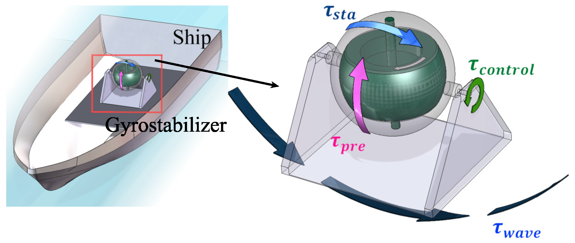
The gyrostabilizer is usually installed inside the cabin of the ship, and its precession axis is perpendicular to the ship’s roll axis, as shown in Figure 1. Its output torque and dynamics can be described as follows [14,21]:

$$\begin{array}{cc}\hfill & {\tau }_{sta}=h_0\dot{\beta }cos\left(\beta \right)\hfill \end{array}$$

(2)

$$\begin{array}{cc}\hfill & J_g\ddot{\beta }+b_1\dot{\beta }+b_2\beta -h_0\dot{\varphi }cos\left(\beta \right)={\tau }_{control}\hfill \end{array}$$

(3)

where $\beta$, $\dot{\beta }$, and $\ddot{\beta }$ indicate the precession angle, angular velocity, and angular acceleration, respectively. ${\tau }_{sta}$ is the stabilizing torque created by the gyrostabilizer. $J_g$ is the inertia in the precession axis. $b_1$ and $b_2$ are the damping and restoring coefficients. $h_0$ is the angular momentum of the gyro rotor. ${\tau }_{control}$ is the control torque applied to the precession axis, which is produced by the motor [30] in general:

$$\left\{\begin{array}{c}{J}_m{\dot{\omega }}_m=C_m{I}_d-T_L-D_m{\omega }_m\hfill \\ L_m{\dot{I}}_d=-C_m{\omega }_m-R_m{I}_d+U_{d0}\hfill \end{array}\right.$$

(4)

The model of the motor is represented in Equation (4), where $J_m$ is the inertia. $C_m$ and $D_m$ denote the motor torque and damping coefficient, respectively. $R_m$ and $L_m$ are the resistance and inductance, respectively. $U_{d0}$ and $I_d$ are the voltage and current, respectively. $C_m{I}_d$ is the electromagnetic torque generated by the motor. Since the motor and the gyrostabilizer’s precession axis are directly connected, $C_m{I}_d={\tau }_{control}$, and ${\omega }_m=\beta$. $T_L$ is the load torque, which is the part to the left of the equal sign in Equation (3).

In summary, the nonlinear dynamics of ship rolling with gyrostabilizers can be described by Equation (5), and it will be used as the simulation model for computing the global linear predictor.

$$\left\{\begin{array}{c}I(\ddot{\varphi },t)+C(\dot{\varphi },t)+K(\varphi ,t)={\tau }_{wave}(\alpha ,t)-{\tau }_{sta}\hfill \\ (J_g+J_m)\ddot{\beta }=C_m{I}_d-(b_1+D_m)\dot{\beta }-b_2\beta +h_0\dot{\varphi }cos\left(\beta \right)\hfill \\ L_m{\dot{I}}_d=-C_m{\omega }_m-R_m{I}_d+U_{d0}\hfill \end{array}\right.$$

(5)

2.2. Global Linear Prediction

As can be seen from (5), the ship roll control system is a significant nonlinear dynamical system, which is quite unfavourable for the stable control of the ship. To cope with the nonlinearity, this section introduces the global linear predictor based on the Koopman operator.

2.2.1. Global Linear Predictor Based on the Koopman Operator

The Koopman operator for autonomous systems is available in the literature [31]. Let us discuss the Koopman operator for controlled dynamics with disturbances. Consider the following dynamics:

$$x^{+}=f(x+w,u)$$

(6)

where $x\in X\subset {\mathbb{R}}^n$, $u\in U\subset {\mathbb{R}}^m$ are vectors of system state, and control, respectively. f is a continuously differentiable function. X, U are tight subsets [32]. Specifically, to enhance the realism of the simulation results, we add measurement noise $w\in {\mathbb{R}}^n$ in the equation of state. Compared with autonomous systems, the state in the future of system (6) depends not only on the current state but on the control applied to it. Therefore, the evolution of the system in the space $\mathcal{H}$ should contain the control. We define the extended state $\chi ={[x,u]}^T$, and the system (6) can be formulated as

$${\chi }^{+}=\mathrm{F}\left(\mathrm{Ø}\right):=\left[\begin{array}{c}f(x+w,\overline{u})\\ \overline{u}\end{array}\right]$$

(7)

where $\overline{u}\left(t\right)=u\left(t^{+}\right)$ is the control sequence applied to the system. $t^{+}$ is the next time of t. The Koopman operator corresponding to (7) can be expressed as

$$\mathcal{K}\left[\mathrm{g}\right(\mathrm{Ø}\left)\right]=\mathrm{g}\left(\mathrm{F}\right(\mathrm{Ø}\left)\right).$$

(8)

Actually, in the space $\mathcal{H}$, the global linear representation of the original dynamics can always be obtained by constructing Koopman operators, even if it is nonlinear [31] (but typically infinite-dimensional).

Further, the Koopman operator can be decomposed into two matrices:

$$\mathcal{K}=\left[\begin{array}{c}{A}_{\infty \times \infty }{B}_{\infty \times m}\end{array}\right]$$

(9)

where $A\in {\mathbb{R}}^{\infty \times \infty }$, $B\in {\mathbb{R}}^{\infty \times m}$ are the transfer matrices of states and control obtained by slicing the Koopman operator, respectively.

Finally, a linear predictor can be constructed:

$$\left\{\begin{array}{c}{z}^{+}=Az+Bu\hfill \\ \widehat{x}=Cz\hfill \end{array}\right.$$

(10)

where $z=\mathrm{g}\left(\mathit{x}\right)\in {\mathbb{R}}^{\infty }$ is the lifted state which is mapped into the higher-dimensional space. $\widehat{x}\in {\mathbb{R}}^n$ is the state restored from the higher-dimensional space. $C\in {\mathbb{R}}^{n\times \infty }$ is the state restoring matrix.

2.2.2. Data Driven Method for the Global Linear Predictor Realization

It is attractive that the Koopman operator makes the evolution of the system in a higher-dimensional space linear. However, it is difficult to compute due to the space being infinite-dimensional. Fortunately, the finite dimensional approximation of the Koopman operator can be achieved by the Extended Dynamic Mode Decomposition [33] (EDMD) method, and it is offline and data-driven. The process is described in detail below.

Firstly, the system (6) should be discretized to prepare the data, and the discrete dynamics can be expressed as

$$x_{k+1}=f(x_k+w_k,u_k)$$

(11)

where $k\in [0,+\infty )$ is the sampling point. $x_k\in X\subset {\mathbb{R}}^n$, $u_k\in U\subset {\mathbb{R}}^m$, $w_k\in {\mathbb{R}}^n$ are sampling values of the system state, control and measurement noise at the kth moment, respectively.

Let $\check{\mathcal{H}}$ be a finite-dimensional function space consisting of a series of scalar observables about $x_k$, where each element is defined as

$$\mathrm{h}({\mathit{x}}_{\mathit{k}}+{\mathit{w}}_{\mathit{k}})={[{\mathrm{h}}_1({\mathit{x}}_{\mathit{k}}+{\mathit{w}}_{\mathit{k}}),{\mathrm{h}}_2({\mathit{x}}_{\mathit{k}}+{\mathit{w}}_{\mathit{k}}),\dots ,{\mathrm{h}}_{\mathrm{N}}({\mathit{x}}_{\mathit{k}}+{\mathit{w}}_{\mathit{k}})]}^{\mathit{T}}$$

(12)

where $\mathrm{h}:{\mathbb{R}}^{\mathit{n}}\to {\mathbb{R}}^{\mathit{N}}$ is the state lifting function.

To preserve the features of the original system maximally when it evolves in the higher-dimensional space, in practice x, and u are included in the computation along with the state lifting function in the following form:

$$\mathbf{H}{({\mathit{x}}_{\mathit{k}}+{\mathit{w}}_{\mathit{k}},{\mathit{u}}_{\mathit{k}}):=[{\mathit{x}}_{\mathit{k}},\mathrm{h}({\mathit{x}}_{\mathit{k}}+{\mathit{w}}_{\mathit{k}}),{\mathit{u}}_{\mathit{k}}]}^{\mathit{T}}.$$

(13)

Then prepare the data. Let the initial state be $x_0\in X$, and the sampling size be K, the control sequence be ${\left\{\begin{array}{c}{u}_k\end{array}\right\}}_{k=1}^K\in U$. The dynamics (6) is solved using the fourth-order Runge–Kutta method [34], and the state, control, and disturbance data are recorded at each time step. The calculation process is described below:

$$x^{+}=x+{\displaystyle \frac{\Delta t}{6}}(k_1+2k_2+2k_3+k_4)$$

(14)

where $k_1=f(x,u)$, $k_2=f\left(x+{\displaystyle \frac{\Delta t}{2}}{k}_1,u\right)$, $k_3=f\left(x+{\displaystyle \frac{\Delta t}{2}}{k}_2,u\right)$, $k_4=f\left(x+\Delta t{k}_3,u\right)$, $\Delta t$ is the sampling time.

Notice that the control value is a random value in U. It makes the data contain as much behavior as possible to improve the estimation. Let ${\mathcal{K}}_T$ be a discrete Koopman operator defined in the space $\check{\mathcal{H}}$, and let the observables of the system state evolve to the next step. Thus, the discrete Koopman operator can be approximated by the following least squares:

$$\underset{{\mathcal{K}}_T}{min}{\displaystyle \sum _{k=1}^K}\left|\right|\mathbf{H}({\mathit{x}}_{\mathit{k}+\mathit{1}},{\mathit{u}}_{\mathit{k}+\mathit{1}})-{\mathcal{K}}_{\mathit{T}}\mathbf{H}({\mathit{x}}_{\mathit{k}},{\mathit{u}}_{\mathit{k}}){\left|\right|}_{\mathit{2}}^{\mathit{2}}.$$

(15)

Actually, the discrete Koopman operator ${\mathcal{K}}_T$ could be decomposed into matrices $A_T$ and $B_T$ (see (9) for details). Unfold (16) as follows:

$$\underset{A_T,B_T,D_T}{min}{\displaystyle \sum _{k=1}^K}\left|\right|z_{k+1}-A_T{z}_k-B_T{u}_k{\left|\right|}_2^2$$

(16)

where $z_k=[x_k;\mathrm{h}\left({\mathit{x}}_{\mathit{k}}\right)]\in {\mathbb{R}}^{(\mathit{n}+\mathit{N})}$ is the extended lifted state. $A_T\in {\mathbb{R}}^{(n+N)\times (N+n)}$, $B_T\in {\mathbb{R}}^{(n+N)\times m}$ are transfer matrices of the state and control, respectively. And ${\mathcal{K}}_T=[A_T,B_T]$.

The state restoring matrix $C_T$ can be solved by

$$\underset{C_T}{min}{\displaystyle \sum _{k=1}^K}\left|\right|x_k-C_T{z}_k{\left|\right|}_2^2$$

(17)

where $C_T\in {\mathbb{R}}^{n\times (n+N)}$.

The discrete Koopman operator can be easily obtained by solving least squares functions such as (Equations (17) and (18)). The pseudo-code of the discrete Koopman operator finite-dimensional approximation algorithm via EDMD can be summarized as Algorithm 1, where “†” denotes the solution of the pseudo-inverse.

Algorithm 1: Global linear predictor

2.3. Model Predictive Control Base on the Koopman Operator

The theory and construction process of the linear predictor based on the Koopman operator is presented in the above. The method provides a linear predictor:

$$\left\{\begin{array}{c}{z}_{k+1}=A_T{z}_k+B_T{u}_k\hfill \\ \widehat{x_k}=C_T{z}_k\hfill \end{array}\right.$$

(18)

where $z_k=[x_k;\mathrm{h}\left({\mathit{x}}_{\mathit{k}}\right)]$, $\mathrm{h}\left({\mathit{x}}_{\mathit{k}}\right)$ is the lifting function defined in (12), and $x_k=[\varphi ;\dot{\varphi };\beta ;\dot{(}\beta );I_d]$ is the state of dynamics of ship rolling. The nonlinear dynamical model (5) can be represented as a state space by means of the linear predictor described above.

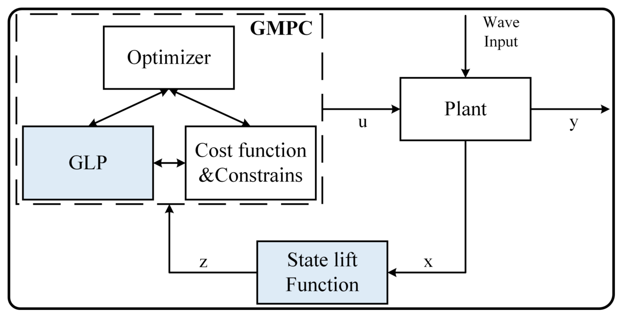
This session presents the construction of the model predictive controller using the global linear predictor based on the Koopman operator. The model predictive control optimizes a specific, user-defined objective function at each time step. Generally, the function of the linear MPC is transformed into a convex quadratic programming problem [35] (QP) to be solved quickly. However, nonlinear MPC may cause a nonconvex optimization problem along with long time consumption and local optimums. The structure of the global linear predictor-based MPC (GMPC) proposed in this paper is shown in Figure 2. Notice that the model used for prediction at each time step is provided by the global linear predictor.

Firstly, the state of the system is being measured at each time step. Then, the lifted state is acquired by the state lifting function. And the global linear predictor based on the Koopman operator is engaged in the scrolling optimization. Finally the optimized control parameters are applied to the plant. The optimization objective function is defined as follows:

$$\left\{\begin{array}{c}\underset{u_i}{min}J=({\displaystyle {\sum }_{i=0}^{N_p-1}}{z}_i^{T}Q{z}_i+u_i^{T}R{u}_i)+z_{N_p}^{T}P{z}_{N_p}\hfill \\ \mathrm{subject}\mathrm{to}\left\{\begin{array}{c}{z}_{i+1}={\mathit{Az}}_i+{\mathit{Bu}}_i,i=0,1,\dots ,N_{p-1}\hfill \\ z_{N_p}\in X_f\hfill \\ u_i\in U\hfill \end{array}\right.\hfill \\ \mathrm{parameters}{\mathit{z}}_{\mathit{0}}=[{\mathit{x}}_{\mathit{0}};\mathrm{h}\left({\mathit{x}}_{\mathit{0}}\right)]\hfill \end{array}\right.$$

(19)

where $Q\in {\mathbb{R}}^{(n+N)\times (n+N)}$, $R\in {\mathbb{R}}^{m\times m}$, $P\in {\mathbb{R}}^{(n+N)\times (n+N)}$ are weight matrices of the process state, control and terminal state, respectively. $X_f$ is the terminal state constraint set, and U is the control constraint set.

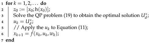
Since the state vector engaged in the scrolling optimization is lifted to the higher-dimensional space instead of the original state, leading to its physical significance becoming unclear. Thus, the actual state $x_k$ of the system at each time step is expanded into $z_k$ to specify the value of its weight matrix. The pseudo-code of the GLP-MPC algorithm can be summarized as Algorithm 2.

Algorithm 2: GLP-MPC

2.4. Control System Stability Analysis

The proposed GMPC is constructed based on the finite-dimensional Koopman predictor given in (18). To guarantee the stability of the closed-loop control system, a Lyapunov-based analysis is presented in this subsection.

Consider the lifted linear prediction model:

$$z_{k+1}=A_T{z}_k+B_T{u}_k$$

(20)

where $z_k\in {\mathbb{R}}^{n+N}$ denotes the lifted state vector and $u_k\in {\mathbb{R}}^m$ is the control input.

The cost function of the proposed GMPC can be written as

$$J\left(k\right)={\displaystyle \sum _{i=0}^{N_p-1}}\left(z_{k+i}^{T}Q{z}_{k+i}+u_{k+i}^{T}R{u}_{k+i}\right)+z_{k+N_p}^{T}P{z}_{k+N_p}$$

(21)

where $Q⪰0$, $R\succ 0$, and $P\succ 0$ denote the state weighting matrix, control weighting matrix, and terminal weighting matrix, respectively.

Assume that:

(A1)

The pair $(A_T,B_T)$ is stabilizable.

(A2)

The terminal weighting matrix P satisfies the discrete-time algebraic Riccati equation.

(A3)

The optimization problem is feasible at the initial sampling instant.

Under these assumptions, define the Lyapunov candidate function as the optimal value function of the MPC problem:

$$V\left(z_k\right)=J^{\ast }\left(z_k\right)$$

(22)

where $J^{\ast }\left(z_k\right)$ denotes the optimal cost obtained by solving the MPC optimization problem at time instant k.

For the optimal control sequence $\{u_k^{\ast },u_{k+1}^{\ast },\cdots ,u_{k+N_p-1}^{\ast }\}$, a feasible control sequence at the next sampling instant can be constructed by shifting the optimal sequence forward and appending the terminal feedback control law. Therefore,

$$V\left(z_{k+1}\right)-V\left(z_k\right)\le -z_k^{T}Q{z}_k-u_k^{T}R{u}_k.$$

(23)

Since $Q⪰0$ and $R\succ 0$, it follows that:

$$V\left(z_{k+1}\right)-V\left(z_k\right)\le 0.$$

(24)

Thus, the Lyapunov function $V\left(z_k\right)$ is non-increasing along the closed-loop trajectories. Moreover,

$$V\left(z_{k+1}\right)-V\left(z_k\right)=0$$

(25)

holds only when

$$z_k=0,u_k=0.$$

(26)

According to the discrete-time Lyapunov stability theorem, the equilibrium point of the lifted prediction system is asymptotically stable. Since the original ship roll states are reconstructed from the lifted states through

$${\widehat{x}}_k=C_T{z}_k,$$

(27)

the asymptotic convergence of $z_k$ implies the asymptotic convergence of the original roll states. Therefore, the proposed GMPC guarantees the closed-loop stability of the ship roll control system.

Remark 1. 

The above stability proof is established in the lifted-state space generated by the Koopman operator. Since the lifting mapping preserves the dominant dynamical characteristics of the original nonlinear system and the reconstruction matrix $C_T$ is bounded, the stability of the lifted linear system can be transferred to the original ship roll dynamics. Therefore, the proposed control framework inherits the computational efficiency of linear MPC while retaining the capability to stabilize the nonlinear roll motion.

3. Results

3.1. Simulation Setup

In this section, we designed numerical simulations to validate the effectiveness of the proposed method, and comparative simulations to verify the advancement and innovation of the system. In detail, to ensure the reliability of the simulation experiment, we made efforts in two ways. On the one hand, the actual parameters of ship’s the own gyrostabilizer are used as the simulation conditions, and the parameters of the boat made in the laboratory are used as the simulation carrier parameters. On the other hand, both regular and irregular long-crested wave environments are simulated and tested. The detailed parameters of the ship and gyrostabilizer are shown in

Table 1. Hydrodynamics of JH-7500 and parameters of the gyrostabilizer.

System	Parameter	Value
Ship (JH-7500)	$L_{oa}$ (m)	7.5
	$B_{wl}$ (m)	3.2
	$\Delta$ (t)	3.7
	$GM$ (m)	0.5
	$I_{xx}+J_{xx}$ ($\mathrm{kg}·{\mathrm{m}}^2$)	1655.11
	$c_1$ ($\mathrm{kg}·{\mathrm{m}}^2/\mathrm{s}$)	258.25
	$c_3$ ($\mathrm{kg}·{\mathrm{m}}^2/\mathrm{s}$)	113.74
	$k_1$ ($\mathrm{kg}·{\mathrm{m}}^2/{\mathrm{s}}^2$)	1054.35
	$k_3$ ($\mathrm{kg}·{\mathrm{m}}^2/{\mathrm{s}}^2$)	−531.15
	$k_5$ ($\mathrm{kg}·{\mathrm{m}}^2/{\mathrm{s}}^2$)	35.32
Gyrostabilizer	$h_0$ ($\mathrm{N}·\mathrm{ms}$)	1000
	$J_g$ ($\mathrm{kg}·{\mathrm{m}}^2$)	1.57
	$b_1$ ($\mathrm{kg}·{\mathrm{m}}^2/\mathrm{s}$)	29.76
	$b_2$ ($\mathrm{kg}·{\mathrm{m}}^2/{\mathrm{s}}^2$)	0.259
	$J_m$ ($\mathrm{kg}·{\mathrm{m}}^2$)	2 × 10−4
	$C_m$ ($\mathrm{kg}·{\mathrm{m}}^2/\mathrm{s}$)	10.875
	$D_m$ ($\mathrm{kg}·{\mathrm{m}}^2/\mathrm{s}$)	0.003
	$R_m$ ($\mathrm{\Omega }$)	0.85
	$L_m$ ($\mathrm{H}$)	0.506

. And all parameters are based on experimental measurements.

Firstly, we conducted numerical simulations under regular wave conditions to verify the effectiveness of the proposed method under ideal conditions. Wave-induced forces under regular wave conditions can be calculated as follows:

$${\tau }_{wave}^{\left(r\right)}\left(t\right)=\Delta GM{\alpha }_r\left(t\right)$$

(28)

where ${\alpha }_r\left(t\right)={\delta }_{r}cos\left({\omega }_{r}t\right)$, ${\delta }_r$, ${\omega }_r$ represent the amplitude and frequency of the wave-induced torque under regular wave conditions, respectively.

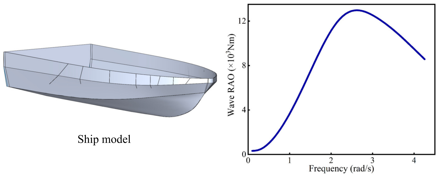
In addition, to validate the effectiveness of the proposed method in a real ocean environment, we computed the response amplitude operator (RAO) for wave-induced moments using potential flow theory. The ship model and computational results are shown in Figure 3.

According to the above results, the wave-induced moment in beam sea conditions can be calculated as

$${\tau }_{wave}^{\left(ir\right)}\left(t\right)={\displaystyle \sum _{j=1}^{N_w}}\sqrt{2S\left(\omega \right)\Delta \omega )}Recos({\omega }_{j}t+Im+{ϵ}_j)$$

(29)

where $N_w$ denotes the number of wave frequencies. $\Delta \omega$ denotes the difference between two neighbouring frequencies. ${ϵ}_j$ denotes the random initial phase. $Re$ and $Im$ denote the real and imaginary parts of the wave moment RAO of the ship. ${\omega }_j$ denotes the wave frequency component. $S\left(\omega \right)$ denotes the wave spectrum. In this paper, the ITTC two-parameter wave spectrum is used:

$$S\left(\omega \right)={\displaystyle \frac{173H_s^2}{T_p^4{\omega }^5}}exp\left({\displaystyle \frac{-691}{T_p^4{\omega }^4}}\right)$$

(30)

where $H_s$ is the significant wave height, $T_p$ is the spectral peak period of the irregular wave, and $\omega$ is the frequency band for simulation. In order to minimize the self-repetition of irregular waves, $\omega$ is sampled from the frequency range $[0,6\pi /T_p]$ with unequal intervals.

More importantly, in order to enhance the credibility of the simulation and further verify the effectiveness of the method, we carried out simulations in a beam sea environment with regular and irregular waves. Furthermore, wave parameters were based on typical sea conditions in the North Atlantic [36], as shown in

Table 2. Sea condition parameters.

Case	Type	${\mathit{H}}_{\mathit{s}}$ ($\mathbf{m}$)	${\mathit{\delta }}_{\mathit{r}}$ ($\mathbf{deg}$)	${\mathit{T}}_{\mathit{p}}$ ($\mathbf{s}$)
1	Regular wave	-	4	10
2	Irregular wave	0.25	-	4.75
3	Irregular wave	0.68	-	6.34
4	Irregular wave	1.12	-	7.92
5	Irregular wave	2.30	-	9.90
6	Irregular wave	3.10	-	11.88

.

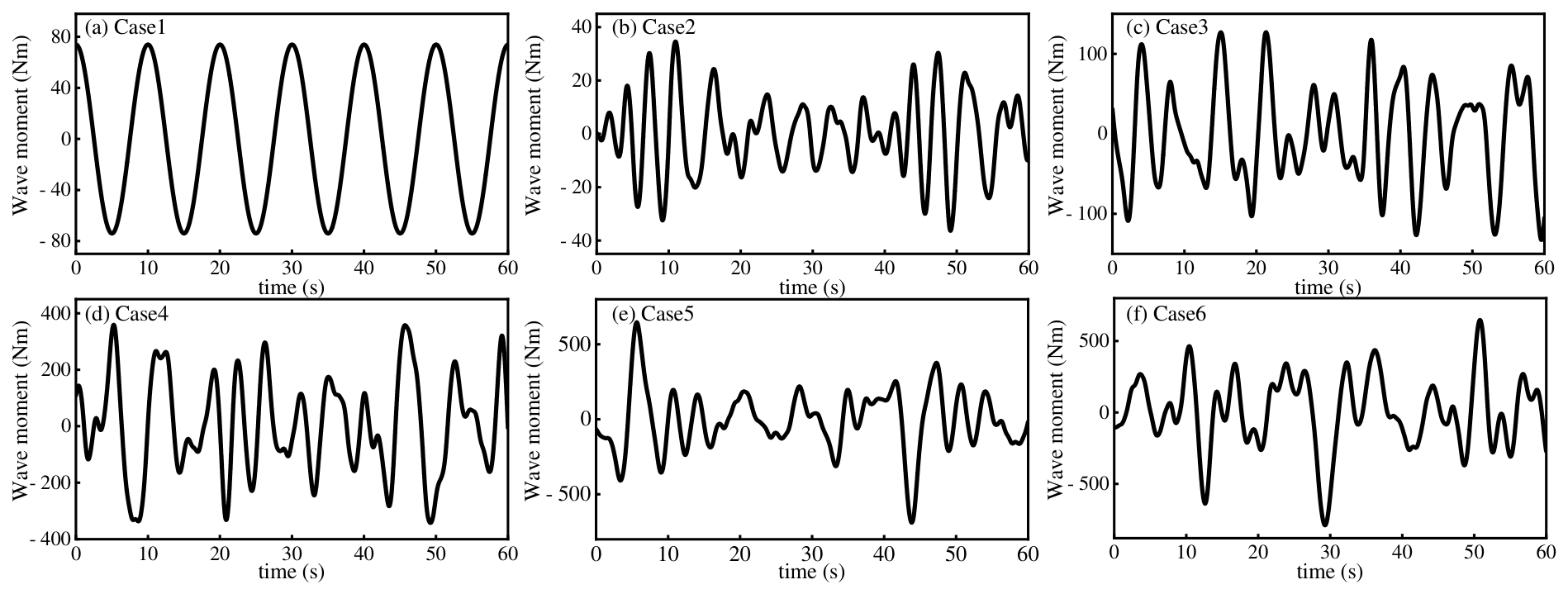
The simulation results for the effects of wave-induced moments on the ship’s roll axis in beam seas are shown in Figure 4.

Under the above conditions, we designed two simulations:

(1)

Linear prediction simulation. The effectiveness of the global linear predictor is verified by comparison with the classical linear prediction algorithm (Algorithm 1).

(2)

Controller comparative simulation. In different wave environments, the control stability and accuracy of the proposed system (Algorithm 2) and the other two classical systems are verified by comparing the three performance indicators.

The abbreviations of the proposed method and other compared methods are listed in

Table 3. Abbreviations of methods.

Abbreviations	Details
LLP	Local linear predictor based on Taylor series.
GLP	Global linear predictor based on the Koopman operator.
LMPC	Model predictive control based on the local linear predictor.
NMPC	Model predictive control based on the nonlinear predictor.
GMPC	Model predictive control based on the global linear predictor.

.

3.2. Linear Predict Simulation

In order to evaluate the effectiveness of the proposed method on system state predictions, we compare its prediction properties with LLP, which is commonly used. Firstly, we construct training datasets and testing datasets under different parameter settings as follows:

• Training: The sampling interval of the training data is set to 0.01 s, step stride is 100, and the sampling period is 10 s. The control data is generated by a sine wave with an amplitude ranging from [1, 10] and a period ranging from [0.35 s, 1.55 s]. The moment applied to the roll axis of the ship, which is calculated using this control data, covers the range of waves-induced moments for the six typical sea conditions shown in Table 2. The state data are obtained from Equation (5) with random initial values.
• Testing: The sampling interval of testing data is set to 0.01 s, step stride is 300, and the sampling period is 3 s. The settings of other parameters are consistent with those of the training phase. Notably, to simulate sensor noise, we added normally distributed noise with standard deviations of [0.02, 0.01, 0.02, 0.01, 0.05] to the testing set during the prediction phase.

In order to verify the sensitivity of various lifting functions to the performance of the predictor, we conducted numerical simulations using Gaussian, polynomial, trigonometric, and mixed observers, respectively. We define the original state variables of the system as $x=[\varphi ,\dot{\varphi },\beta ,\dot{\beta },I_d]$. The lifting functions are expressed as follows:

$${\mathrm{h}}_{{\mathrm{G}}_{\mathrm{i}}}=\exp \left({\displaystyle \frac{-\left|\right|{\mathit{x}}_{\mathit{k}}-{\mathit{r}}_{{\mathit{b}}_{\mathit{i}}}{\left|\right|}_{\mathit{2}}^{\mathit{2}}}{\mathit{2}}}\right)$$

(31)

$${\mathrm{h}}_{{\mathrm{P}}_{\mathrm{i}}}={\displaystyle \prod _{\mathit{j}=\mathit{1}}^{\mathit{n}}}{\mathit{x}}_{\mathit{j}}^{{\mathit{ff}}_{\mathit{ij}}}$$

(32)

$${\mathrm{h}}_{{\mathrm{T}}_{\mathrm{i}}}=\sin \left({\mathit{k}}_{\mathit{ij}}^{\mathit{T}}\mathit{x}\right)$$

(33)

$${\mathrm{h}}_{{\mathrm{M}}_{\mathrm{i}}}={[\mathit{x},{\mathrm{h}}_{{\mathrm{G}}_{\mathrm{i}}},{\mathrm{h}}_{{\mathrm{P}}_{\mathrm{i}}},{\mathrm{h}}_{{\mathrm{T}}_{\mathrm{i}}}]}^{\mathrm{T}}$$

(34)

where ${\mathrm{h}}_{{\mathrm{G}}_{\mathrm{i}}},{\mathrm{h}}_{{\mathrm{P}}_{\mathrm{i}}},{\mathrm{h}}_{{\mathrm{T}}_{\mathrm{i}}},{\mathrm{h}}_{{\mathrm{M}}_{\mathrm{i}}}$ represent the i-th ($i=1:N$) Gaussian observer, polynomial observer, trigonometric observer, and mixed observer, respectively. $r_{b_i}$ denotes the center of the kernel function for the i-th lifting function. ${\alpha }_{ij}$ denotes the power-index vector of the j-th ($j=1:5$) primitive state in the i-th lifting function. $k_{ij}$ denotes the periodicity feature of the j-th primitive state in the i-th lifting function.

In addition, the state lifting dimension is also one of the important parameters of GLP, as it directly affects the predictor’s sensitivity to a nonlinear dynamical system. As is well known, the average RMSE between the predicted state and the true state can effectively be used to characterize the accuracy of the linear predictor. Therefore, we conducted ablation simulation experiments to test the state RMSE performance of system prediction under different parameter settings. The parameter range of the state lifting dimension was set from 10 to 100, with unequal interval sampling. We ran 100 experiments for each parameter and recorded the average RMSE of the repeated simulation experiments, as shown in

Table 4. Comparison of predictions for different lifting dimensions.

Lifting Dimension	Average RMSE (%)
	GLP (Ours)				LLP
	Gaussian	Polynomial	Trigonometric	Mixed	-
$N=10$	4.90	7.67	5.15	6.42	18.02
$N=30$	4.65	8.05	4.76	6.33	19.35
$N=50$	4.11	7.13	4.96	5.84	18.27
$N=100$	3.10	6.69	3.98	6.13	18.66

.

It can be observed from Table 4 that the prediction performance of all GLP-based predictors is significantly superior to that of LLP under all tested parameter settings. Regardless of the lifting dimension, the average RMSE of the four lifting-function configurations remains substantially lower than that of LLP, demonstrating the effectiveness of the proposed lifting-based linear prediction framework in capturing the nonlinear dynamics of the roll stabilization system. Furthermore, as the lifting dimension N increases, the average prediction RMSE generally exhibits a decreasing trend, although the reduction is not strictly monotonic for every lifting function. This indicates that a larger lifted state space provides richer observable information and enables the predictor to characterize the underlying nonlinear dynamics more accurately.

Comparing different lifting functions, the Gaussian observer consistently achieves the best prediction accuracy among all tested configurations. Its average RMSE decreases from 4.90% at $N=10$ to 3.10% at $N=100$, indicating that Gaussian radial basis functions possess strong local approximation capability for nonlinear roll dynamics. The trigonometric observer provides the second-best performance, suggesting that periodic basis functions are effective in describing the oscillatory characteristics of ship roll motion. Although the polynomial observer can partially capture the nonlinear restoring moments of the system, its prediction accuracy is inferior to Gaussian and trigonometric observers, especially at lower lifting dimensions. The mixed observer combines multiple basis-function types and achieves stable prediction performance over different lifting dimensions, but its accuracy does not surpass that of the Gaussian observer in the considered case. Based on the above results, in the subsequent numerical simulation phase, we selected the Gaussian observer as the lifting function. Simultaneously, the state lifting dimension was set to 100.

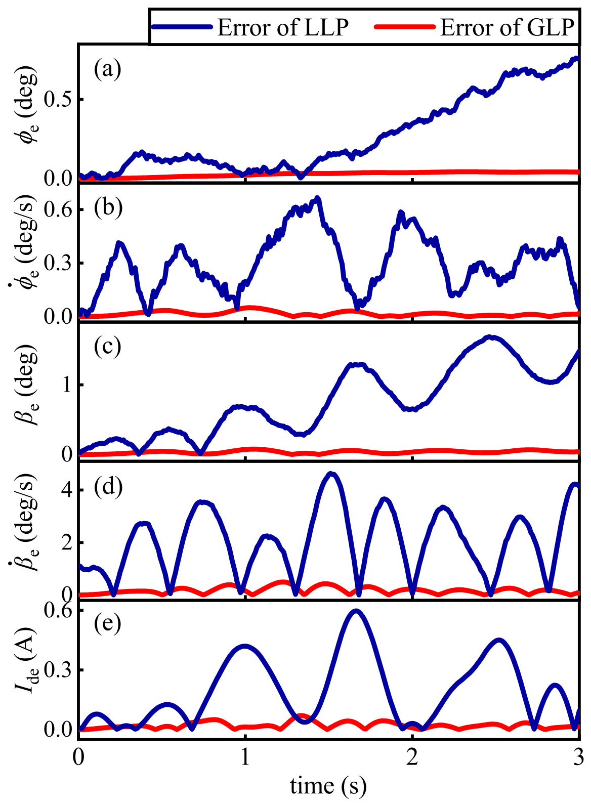
Furthermore, we conduct a comparison experiment between the proposed algorithm and the commonly used LLP. We select the ship rolling angle error (${\varphi }_e$), rolling angular velocity error (${\dot{\varphi }}_e$), gyro precession angle error (${\beta }_e$), precession angular velocity error (${\dot{\beta }}_e$) and motor current error ($I_{de}$) for estimating accuracy comparison parameters. The simulation experiment results are shown in Figure 5.

As can be seen from the figure, the prediction error of the GLP algorithm is lower than that of the LLP algorithm for all five state variable estimates, which indicates that the prediction results of the GLP algorithm are closer to the true values. This is because the LLP algorithm typically expands linearly around the system’s equilibrium point and ignores higher-order subterms, which cannot accurately represent the system behavior when the system deviates from the equilibrium point, while the GLP algorithm achieves accurate modeling of nonlinear systems through the behavioral data of the nonlinear system in all state spaces, and thus can characterize the system more accurately. Therefore, the algorithm’s state estimation results perform better regardless of the system’s arbitrary position in the state space.

3.3. Controller Comparative Simulation Experiment

In order to further evaluate the accuracy of the proposed algorithm in ship rolling control, we constructed a GMPC controller using the GLP algorithm (see Algorithm 2 and Figure 2 for details), and carried out control simulations in beam sea environments (including regular and irregular waves), respectively.

$$\eta ={\displaystyle \frac{{\varphi }_N-{\varphi }_P}{{\varphi }_N}}\times 100\%$$

(35)

where ${\varphi }_N$ denotes the standard deviation of the ship’s free rolling (without gyrostabilizers) angle and ${\varphi }_P$ denotes the standard deviation of the ship’s rolling angle with controlled gyrostabilizers.

In addition, we constructed LMPC and NMPC for comparison simulations under the same control parameters to verify the advantages of GMPC in terms of control accuracy and real-time performance. Both GMPC and LMPC are solved by the open source quadratic programming tool in MATLAB 2024a, while NMPC is solved using the CASAdi toolkit [37]. The controller parameter settings are shown in

Table 5. Controller parameters.

Parameters	LMPC	NMPC	GMPC
Sampling time	0.01 s
Simulation time	60 s (6000 steps)
Prediction horizon	3 steps
Weight matrix Q	diag$(10,0,0,0,3)$		diag$(10,0,0,0,3,0,\dots ,0)$
Weight matrix R	0.05
Weight matrix P	diag$(10,0,0,0,3)$		diag$(10,0,0,0,3,0,\dots ,0)$

.

Notice that the parameters of the four controllers in Table 5 are the same except for the weight matrices Q and P. Since the state vector used for rolling optimization in GMPC is concatenated by the original state vector $x\in {\mathbb{R}}^5$, the lifted state vector $\mathrm{h}\left(\mathit{x}\right)\in {\mathbb{R}}^{100}$, and the control vector $u\in {\mathbb{R}}^1$ (see (13) for details). Therefore, the dimension of the state vector is set to be 106 (i.e., $(5+100+1)$), which is different from the other two controllers. In order to maintain maximum consistency of the parameters, we set the parameters related to the original system state (the first 5) in the Q and P weight matrices of the GMPC to the same values as those used in the other two controllers.

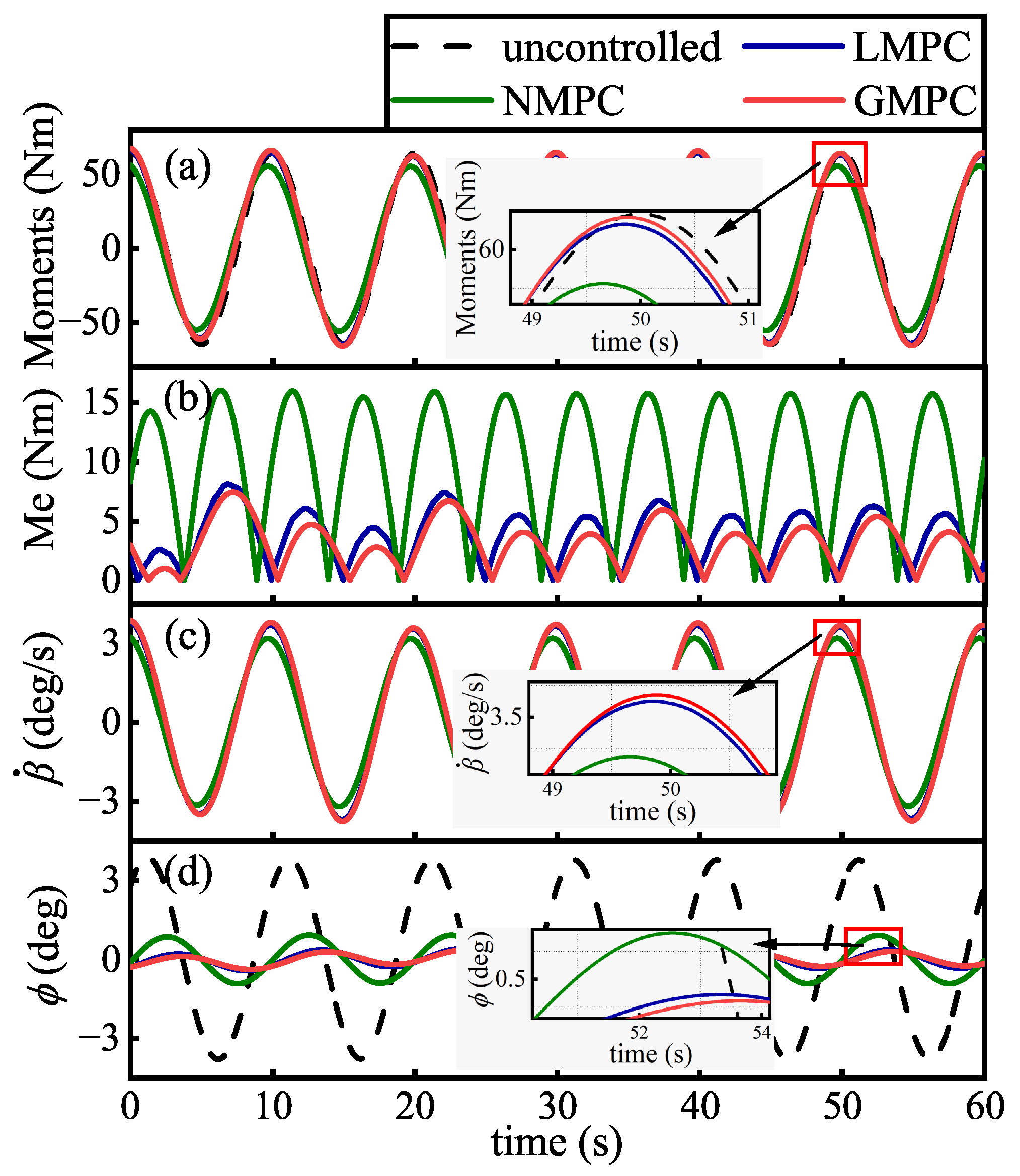
With the above parameter settings, the simulations were carried out under the six wave environments (including regular and irregular waves) shown in Table 2. Where the regular wave represents the ideal wave environment, while the irregular wave represents the real sea conditions. We chose the moment error ($M_e$), the gyro precession angular velocity ($\dot{\beta }$), and the ship roll angle ($\varphi$) to characterize the accuracy of the controller. Here, $M_e$ represents the absolute value of the difference between the wave excitation moment and the gyro stabilizing moment. Hence, its periodic characteristics will be distinct from those of other curves in the figure. These parameters can characterize the control robustness of the system in different environments, and lower torque error, larger gyro precession angular velocity, and smaller ship roll angle indicate stronger resistance to wave interference and higher stability of the system. The simulation results in the regular wave environment are shown in Figure 6.

As can be seen in Figure 6, when the ship without gyrostabilizers is operating in a regular wave environment, the ship’s free rolling angle can be up to 4 degrees (black solid line in Figure 6d). And with the controller, the torque error is reduced, the gyro precession angular velocity is increased, and the system stability is improved. The gyro precession angular velocity is positively correlated with its output stabilizing torque (see (2) for details), its increase improves the system’s ability to resist wave disturbances and thus reduces the torque error. The rolling angle of the ship is obviously reduced (Figure 6d), which indicates that the stabilizing torque generated by the gyrostabilizer cancels out part of the system disturbance. Consequently, the actual disturbance to the ship is smaller than that of the ambient wave disturbance, and the ship’s motion is smoother.

Moreover, It can be seen from Figure 6a that the control moments generated by the three controllers exhibit the same shape and trend as the wave-induced moment, yet the moment generated by the GMPC is closer to the wave-induced moment. This is also evident in Figure 6b, where the GMPC exhibits a smaller moment error of less than 5 Nm. This is primarily because, under the influence of the GMPC, the gyro produced a higher precession angular velocity (Figure 6c). This indicates that the gyrostabilizer based on the GMPC algorithm has better efficacy and ship motion stability. As can be seen from Figure 6d, the rolling angle of the ship of GMPC controller fluctuates around 0 degrees with small amplitudes, the gyrostabilizer produces accurate stabilizing torque, and the ship realizes small amplitude rolling motion in a regular wave environment. From the combined results in Figure 6, it is clear that the GLP proposed in Algorithm 1 does provide accurate state predictions for the controller. Although the physical significance of the system states that are mapped into the higher-dimensional space is not clear, these results confirm that the proposed algorithm’s mapping relationship from the lower-dimensional nonlinear space to the higher-dimensional linear space is correct.

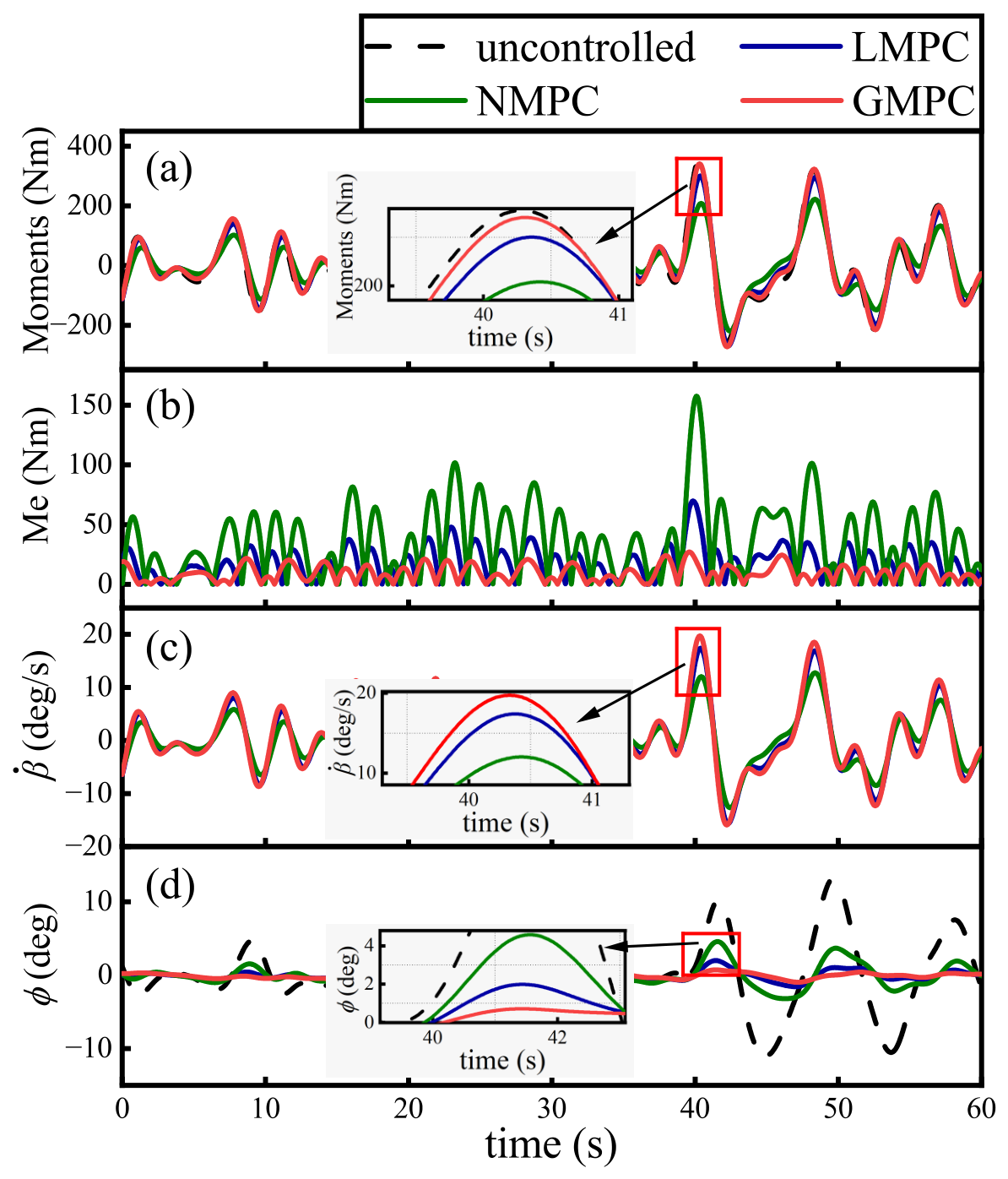
We verified the control accuracy in irregular wave environments that are closer to the real sea conditions. The parameters of the irregular wave environments are shown as Case 2 to Case 6 in Table 2, which represents typical sea conditions from Level I and Level V, respectively.

Figure 7a shows the wave-induced moment and control moment under irregular wave conditions (Case 4). Compared to regular wave conditions, the amplitude and frequency of the wave disturbance moment vary over time under irregular wave conditions. Nevertheless, the gyro-stabilizing moment of the GMPC remains close to the wave-induced moment. In Case 4, the error between the gyro stabilization moments of NMPC and LMPC and the wave disturbance moments increases, exceeding 150 Nm. While the algorithm in this paper maintains global robustness, as shown in the local magnification of Figure 7c, the GMPC-controlled gyrostabilizer generates a larger precession angular velocity, thereby producing a larger stabilization moment. Even during the period of most severe disturbance (40–42 s), the GMPC is still able to maintain control accuracy. Furthermore, Figure 7d reports the ship’s roll angle under irregular wave disturbances, showing that the GMPC exhibits a much smaller roll angle amplitude and consistently maintains a high stabilization efficiency.

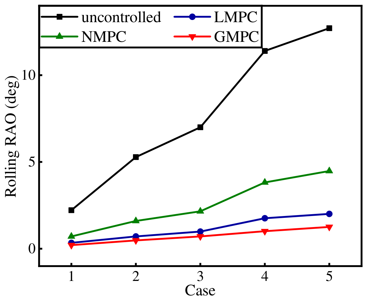
Furthermore, to analyze the robustness of the proposed method, we conducted multiple numerical simulations over a wider range of wave parameters and used the response amplitude operator to characterize the rolling behavior of uncontrolled and controlled ships under various irregular wave conditions. The results are shown in Figure 8.

Figure 8 presents the roll responses of the ship under five regular-wave conditions with different wave parameters. It can be clearly observed that the roll motion of the uncontrolled ship increases significantly as the sea state becomes more severe. Specifically, the rolling RAO rises continuously from Sea State 1 to Sea State 5, indicating that stronger wave excitation introduces larger external disturbance moments to the vessel. Such excessive roll motion not only degrades mission performance but also poses a serious threat to navigation safety and onboard operational reliability.

When the control systems are activated, all three controllers effectively suppress the roll motion to different extents. Compared with the uncontrolled case, the TMPC, NMPC, and GMPC controllers all achieve considerable reductions in rolling amplitude under every sea-state condition, demonstrating their capability to mitigate wave-induced disturbances. More importantly, even under the harshest sea conditions, the controlled roll angles remain below 5 deg, indicating that the active stabilization system can maintain satisfactory roll performance throughout the entire operating range considered in this study.

A further comparison among the three control strategies reveals that the proposed GMPC consistently achieves the lowest rolling RAO under all wave conditions. As the wave intensity increases, the superiority of GMPC becomes increasingly evident. This result indicates that the Koopman-based predictor can capture the nonlinear roll dynamics more accurately than the linear predictor employed by TMPC, while simultaneously avoiding the high computational burden associated with the nonlinear optimization process of NMPC. Consequently, the GMPC controller generates more effective control actions and provides superior roll attenuation performance across a wide range of sea states.

Overall, the results demonstrate that the proposed GMPC not only preserves the robustness of model predictive control under varying wave environments but also achieves the best roll reduction performance among the considered control strategies. Therefore, it provides an effective solution for ship roll stabilization in both moderate and severe sea conditions.Moreover, the performance gap between GMPC and the other controllers becomes more pronounced as the sea state increases, suggesting that the proposed Koopman-based predictor possesses stronger disturbance-rejection capability and better adaptability to highly nonlinear roll dynamics under severe wave conditions.

Finally, we conducted a comprehensive and systematic simulation. Ship motion and computational time consumption in the six wave environments are recorded in

Table 6. System control properties.

Controller	Case	Rolling Standard (deg)	Control Efficiency (%)	Time Cost on Each Step (ms)
uncontrolled	1	3.80	-	-
	2	2.22	-	-
	3	5.28	-	-
	4	7.00	-	-
	5	11.40	-	-
	6	12.71	-	-
LMPC	1	0.37	90.06	0.41
	2	0.34	84.73	0.48
	3	0.71	86.56	0.45
	4	0.99	85.82	0.47
	5	1.76	84.59	0.51
	6	2.01	84.19	0.48
NMPC	1	0.94	75.17	19.85
	2	0.71	67.75	21.40
	3	1.60	69.82	25.26
	4	2.16	69.13	20.63
	5	3.82	66.59	20.06
	6	4.48	64.73	19.96
GMPC	1	0.31	91.75	0.38
	2	0.21	90.54	0.40
	3	0.48	90.90	0.45
	4	0.71	89.85	0.34
	5	1.01	91.14	0.44
	6	1.26	90.08	0.45

, where the data are the average numerical results of 10 repeated simulations with random wave slices and random state initial values. As can be seen, under different wave environments, compared with the free rolling motion of the ship, the amplitude and standard deviation of the ship’s rolling angle based on the three control methods are reduced to different degrees, and the stability of the ship’s motion is improved. In particular, the amplitude and standard deviation of the ship’s roll angle under GMPC are significantly lower than those of the remaining two, and the control efficiency is significantly improved.

Table 6 summarizes the roll stabilization performance and computational efficiency of different controllers under six wave conditions. The reported values are the average results of 10 independent simulations with randomly selected wave segments and random initial states. To further evaluate the practical applicability of the controllers, measurement noise was introduced into the feedback states during the simulations.

It can be observed that all three control strategies significantly reduce the roll motion compared with the uncontrolled case. As the wave environment becomes more severe, the rolling standard deviation of the uncontrolled ship increases continuously from 3.80 deg in Case 1 to 12.71 deg in Case 6, indicating that stronger wave disturbances lead to larger roll motions and deteriorate ship stability. After the controllers are activated, the rolling standard deviations are substantially reduced under all sea conditions, demonstrating the effectiveness of active roll stabilization.

From the perspective of control efficiency, the proposed GMPC consistently achieves the best performance among all considered methods. In the regular-wave environment (Case 1), GMPC attains a roll reduction efficiency of 91.75%, which is higher than that of LMPC (90.06%) and significantly higher than that of NMPC (75.17%). More importantly, when transitioning from the regular-wave condition to the irregular-wave conditions (Cases 2–Case 6), the control efficiencies of LMPC and NMPC exhibit noticeable degradation. This phenomenon can be attributed to the combined influence of irregular environmental disturbances and measurement noise, which introduces larger prediction errors and reduces control accuracy. In contrast, the proposed GMPC maintains a control efficiency of approximately 90% across all irregular-wave conditions, indicating strong robustness against both wave uncertainty and sensor noise.

The computational results further highlight the advantages of GMPC for real-time implementation. The average computational cost of GMPC remains below 0.5 ms per control step for all test cases, which is comparable to that of LMPC and significantly lower than that of NMPC. Specifically, the average computation time of NMPC exceeds 20 ms in all scenarios, whereas the control sampling interval adopted in this study is only 10 ms. Consequently, the nonlinear optimization problem cannot be solved within a single control cycle, resulting in delayed control actions and degraded stabilization performance. This explains why NMPC achieves lower control efficiency despite explicitly considering the nonlinear dynamics of the system.

In contrast, by transforming the nonlinear roll dynamics into a lifted linear prediction model through the Koopman operator, GMPC preserves the computational efficiency of linear MPC while retaining the capability to characterize nonlinear system behavior. Therefore, the proposed method simultaneously achieves superior roll suppression performance, strong robustness to disturbances and measurement noise, and real-time computational capability, making it particularly suitable for practical ship roll stabilization applications.

In summary, the GMPC algorithm provides effective state estimation and real-time performance, which meets the requirements of practical applications.

4. Discussion

4.1. Influence of Koopman Lifting Parameters

The prediction performance of the proposed GMPC framework is closely related to the design of the Koopman lifting space. Therefore, the effects of both lifting functions and lifting dimensions were systematically investigated. The results indicate that all Koopman-based predictors achieve substantially lower prediction errors than the conventional linear predictor, confirming the effectiveness of lifting nonlinear dynamics into a higher-dimensional observable space.

Among the tested lifting functions, the Gaussian observer consistently provides the lowest prediction RMSE, while the polynomial and trigonometric observers exhibit slightly inferior performance. This result suggests that Gaussian basis functions possess stronger local approximation capability for the nonlinear roll dynamics considered in this study. Furthermore, the average prediction RMSE generally decreases as the lifting dimension increases, indicating that a richer observable space can capture more nonlinear dynamical characteristics. However, the performance improvement gradually diminishes at higher lifting dimensions, while the computational complexity continues to increase. Therefore, a moderate lifting dimension is preferred to balance prediction accuracy and computational efficiency.

4.2. Robustness Under Wave Disturbances and Measurement Noise

The simulation results under both regular and irregular wave conditions demonstrate the robustness of the proposed controller. As the sea state becomes more severe, the roll motion of the uncontrolled ship increases significantly, highlighting the necessity of active roll stabilization. Under all tested conditions, the three MPC-based controllers effectively suppress the roll response and maintain the roll angle within an acceptable range.

To further evaluate practical applicability, measurement noise was introduced into the feedback states. Under the combined influence of environmental uncertainty and sensor noise, both LMPC and NMPC exhibit noticeable reductions in control efficiency, particularly in irregular-wave environments. In contrast, GMPC maintains approximately 90% roll reduction efficiency across all test cases. This observation indicates that the Koopman predictor retains sufficient prediction accuracy even in the presence of noisy measurements and uncertain disturbances, thereby providing enhanced robustness for practical marine applications.

4.3. Control Effectiveness and Real-Time Capability

Compared with LMPC and NMPC, the proposed GMPC achieves superior roll stabilization performance while maintaining extremely low computational cost. The results show that GMPC consistently produces the lowest roll standard deviation and the highest control efficiency under all considered sea states.

An important observation is that the average computation time of NMPC exceeds 20 ms per control step, whereas the sampling interval adopted in this study is only 10 ms. Consequently, the nonlinear optimization cannot be completed within a single control cycle, leading to delayed control actions and degraded control performance. Although NMPC explicitly considers nonlinear system dynamics, its computational burden limits its practical applicability for real-time implementation.

By contrast, GMPC requires less than 0.5 ms per control step, which is comparable to LMPC while achieving significantly better roll suppression performance. This advantage originates from the Koopman-based lifting strategy, which transforms the nonlinear prediction problem into a linear MPC framework. Therefore, the proposed method successfully combines the computational efficiency of LMPC with the nonlinear representation capability of NMPC, making it particularly suitable for real-time ship roll stabilization systems.

4.4. Limitations and Future Work

Although the proposed GMPC framework demonstrates promising performance, several limitations remain. First, the Koopman operator is identified offline using simulation-generated datasets, and its prediction accuracy depends on the quality and coverage of the training data. Second, the present study focuses on roll stabilization and does not explicitly consider the coupling effects among the six degrees of freedom of ship motion. Finally, all validations are conducted through numerical simulations. Future work will focus on adaptive Koopman learning, six-degree-of-freedom motion control, and experimental verification through hardware-in-the-loop and physical model tests.

5. Conclusions

This paper proposed a Gaussian lifting-based model predictive control framework for ship roll stabilization. By employing the Koopman operator, nonlinear roll dynamics were transformed into a lifted linear state-space representation, enabling efficient prediction and control within a linear MPC framework. A Lyapunov-based analysis was provided to guarantee the stability of the closed-loop system.

Comprehensive simulations under regular and irregular wave conditions demonstrated that the proposed GMPC achieves superior roll reduction performance, stronger robustness to environmental disturbances and measurement noise, and significantly lower computational cost than both LMPC and NMPC. In particular, the average computation time remained below 0.5 ms per control step while maintaining approximately 90% roll reduction efficiency across all tested sea states. These results indicate that the proposed method provides an effective and computationally efficient solution for real-time ship roll stabilization. Future work will focus on adaptive Koopman learning and experimental validation in realistic marine environments.

References

1. Geng, Y.; Guo, M.; Guo, H.; Chen, H. Safety range in bridge areas based on the influence of cross flow on ship navigation. Ocean Eng. 2023, 281, 114649. [Google Scholar] [CrossRef]
2. Handschel, S.; Feder, D.F.; Abdel-Maksoud, M. Estimation of ship roll damping-A comparison of the decay and the harmonic excited roll motion technique for a post panamax container ship. In Proceedings of the 12th International Conference on the Stability of Ships and Ocean Vehicles, Glasgow, UK, 2015; University of Strathclyde Publishing: Glasgow, UK, 2015; pp. 475–488. [Google Scholar] [CrossRef]
3. Matsui, S. A new mathematical hull-form with 10-shape parameters for evaluation of ship response in waves. J. Mar. Sci. Technol. 2022, 27, 508–521. [Google Scholar] [CrossRef]
4. Katayama, T.; Matsuoka, M.; Adachi, T.; Ikushima, K. Effects of half breadth to draught ratio of hull under water surface on bilge-keel roll damping component. Ocean Eng. 2019, 188, 106283. [Google Scholar] [CrossRef]
5. Thor, F. (Ed.) Handbook of Marine Craft Hydrodynamics and Motion Control; Wiley: Hoboken, NJ, USA, 2012. [Google Scholar] [CrossRef]
6. Rezaei, A.; Tabatabaei, M. Ship roll stabilization using an adaptive fractional-order sliding mode controller. Ocean Eng. 2023, 287, 115883. [Google Scholar] [CrossRef]
7. Xu, W.; Jiao, J.; Xu, G.; Zhang, M.; Zou, Y. Intelligent control of flap-type fin stabilizer for ship roll motion reduction. Ocean Eng. 2025, 323, 120630. [Google Scholar] [CrossRef]
8. Arunkumar, A.; Chang, W.J.; Lee, Y.C.; Lin, Y.H.; Li, L.; Aslam, M.S. Fin Stabilizer-Based Finite-Time H Interval Type-2 Fuzzy Synthesis for Ship Rolling Motion with Bouc–Wen Hysteresis Under Imperfect Premise Matching. IEEE Trans. Fuzzy Syst. 2026; Early Access.
9. Liu, C.; Guo, W.; Sun, T. RLOS-based path following with event-triggered roll motion control for underactuated ship using rudder. Ocean Eng. 2023, 269, 113592. [Google Scholar] [CrossRef]
10. Zhang, Z.; Zou, Z.; Yang, J.; Zhang, X. Nonlinear hydrodynamic model based course control and roll stabilization by taking rudder and propeller actions. Ocean Eng. 2022, 263, 112377. [Google Scholar] [CrossRef]
11. Hariharan, G.; Sathiyaseelan, D. Efficient spectral methods for a class of unsteady-state free-surface ship models using wavelets. Z. Angew. Math. Phys. 2017, 68, 31. [Google Scholar] [CrossRef]
12. Hariharan, G.; Rajaraman, R.; Sathiyaseelan, D. Wavelet based spectral algorithm for nonlinear dynamical systems arising in ship dynamics. Ocean Eng. 2016, 126, 321–328. [Google Scholar] [CrossRef]
13. Qin, L.; Zhang, S.; Zhong, Q.; Nan, X.; Wang, J. Enhancing ship roll reduction using LSTM-based disturbance prediction and sliding mode control. J. Control Decis. 2025, 1–12. [Google Scholar] [CrossRef]
14. Hu, L.; Zhang, M.; Yu, X.; Yuan, Z.M.; Li, W. Real-time control of ship’s roll motion with gyrostabilisers. Ocean Eng. 2023, 285, 115348. [Google Scholar] [CrossRef]
15. Pourmohammadi, M.J.; Eftekhari, M. Vibration control of FG-pipe conveying fluid using a nonlinear absorber with nonlinear damping in longitudinal direction. Mech. Syst. Signal Process. 2025, 223, 111875. [Google Scholar] [CrossRef]
16. Cao, Y.; Li, T.; Hao, L.Y.; Gao, X. Nonlinear Antiswing Control of Shipboard Boom Cranes Using MPC-Based Auto-Tuning Mechanism With Full State Constraints. IEEE Trans. Intell. Transp. Syst. 2023, 25, 2281–2292. [Google Scholar] [CrossRef]
17. Ortega, R.; Cisneros, R.; Wang, L.; van der Schaft, A. Indirect adaptive control of nonlinearly parameterized nonlinear dissipative systems. Int. J. Robust Nonlinear Control 2022, 32, 5105–5119. [Google Scholar] [CrossRef]
18. Rajput, J.; Khan, H.Z.I. Nonlinear Control Allocation Using a Piecewise Multilinear Representation. IEEE Trans. Aerosp. Electron. Syst. 2023, 59, 5314–5323. [Google Scholar] [CrossRef]
19. Taskin, M.; Ahan, A.O. Input saturated H optimal control to mitigate DTMB 5415 combatant roll motion using anti roll gyro stabilizer. Ocean Eng. 2024, 305, 117913. [Google Scholar] [CrossRef]
20. Kuseyri, S. Constrained H control of gyroscopic ship stabilization systems. Proc. Inst. Mech. Eng. Part M J. Eng. Marit. Environ. 2020, 234, 634–641. [Google Scholar] [CrossRef]
21. Song, K.S.; Kim, S.M.; Kwak, M.K.; Zhu, W. Development of a control algorithm for active control of rolling motion of a ship using a gyrostabilizer. Ocean Eng. 2023, 280, 114669. [Google Scholar] [CrossRef]
22. Dahdah, S.; Forbes, J.R. Closed-loop Koopman operator approximation. Mach. Learn. Sci. Technol. 2024, 5, 025038. [Google Scholar] [CrossRef]
23. Lu, T.; Feng, J.; Su, J.; Han, Y.; Guo, Q. System identification based on sparse approximation of Koopman operator. Eur. Phys. J. Spec. Top. 2024, 234, 571–584. [Google Scholar] [CrossRef]
24. Švec, M.; Ileš, Š.; Matuško, J. Predictive Direct Yaw Moment Control Based on the Koopman Operator. IEEE Trans. Control Syst. Technol. 2023, 31, 2912–2919. [Google Scholar] [CrossRef]
25. Li, W.; Zhou, H. Constrained Nonlinear MPC with Rudder-Roll Stabilization for Integrated Path Following and Collision Avoidance in Underactuated Surface Vessels. J. Mar. Sci. Eng. 2025, 13, 468. [Google Scholar] [CrossRef]
26. Zhu, Y.; Su, S.; Qian, Y.; Chen, Y.; Tang, W. Parameter Optimization for Ship Antiroll Gyros. Appl. Sci. 2020, 10, 661. [Google Scholar] [CrossRef]
27. Sathyaseelan, D.; Hariharan, G.; Kannan, K. Parameter identification for nonlinear damping coefficient from large-amplitude ship roll motion using wavelets. Beni-Suef Univ. J. Basic Appl. Sci. 2017, 6, 138–144. [Google Scholar] [CrossRef]
28. Rajaraman, R.; Hariharan, G. Estimation of roll damping parameters using Hermite wavelets: An operational matrix of derivative approach. Ocean Eng. 2023, 283, 115031. [Google Scholar] [CrossRef]
29. Zhang, Z.; Yang, J.; Zhang, H.; Zou, Z.; Zhang, X. Numerical study on mean wave drift forces and moment of ships using Rankine panel method in frequency domain. Ocean Eng. 2023, 283, 114986. [Google Scholar] [CrossRef]
30. Yañez-Badillo, H.; Beltran-Carbajal, F.; Rivas-Cambero, I.; Favela-Contreras, A.; Arroyo-Nuñez, J.H.; Balderas-Gutierrez, J.N. Enhanced Output Tracking Control for Direct Current Electric Motor Systems Using Bio-Inspired Optimization. Machines 2023, 11, 1006. [Google Scholar] [CrossRef]
31. Korda, M.; Mezić, I. Linear predictors for nonlinear dynamical systems: Koopman operator meets model predictive control. Automatica 2018, 93, 149–160. [Google Scholar] [CrossRef]
32. Lu, E.; Xue, J.; Chen, T.; Jiang, S. Robust trajectory tracking control of an autonomous tractor-trailer considering model parameter uncertainties and disturbances. Agriculture 2023, 13, 869. [Google Scholar] [CrossRef]
33. Bruder, D.; Fu, X.; Vasudevan, R. Advantages of bilinear Koopman realizations for the modeling and control of systems with unknown dynamics. IEEE Robot. Autom. Lett. 2021, 6, 4369–4376. [Google Scholar] [CrossRef]
34. Li, X.; Wang, Z.; Ma, Q.; Ding, X. Conservative Continuous-Stage Stochastic Runge–Kutta Methods for Stochastic Differential Equations. Fractal Fract. 2023, 7, 83. [Google Scholar] [CrossRef]
35. Mirzaeva, G.; Mo, Y. Model predictive control for industrial drive applications. IEEE Trans. Ind. Appl. 2023, 59, 7897–7907. [Google Scholar] [CrossRef]
36. Hersbach, H.; Bell, B.; Berrisford, P.; Hirahara, S.; Horányi, A.; Muñoz-Sabater, J.; Nicolas, J.; Peubey, C.; Radu, R.; Schepers, D.; et al. The ERA5 global reanalysis. Q. J. R. Meteorol. Soc. 2020, 146, 1999–2049. [Google Scholar] [CrossRef]
37. Andersson, J.A.; Gillis, J.; Horn, G.; Rawlings, J.B.; Diehl, M. CasADi: A software framework for nonlinear optimization and optimal control. Math. Program. Comput. 2019, 11, 1–36. [Google Scholar] [CrossRef]
Figure 1. Ship-gyrostabilizer system construction.
Oceans 07 00053 g001
Figure 2. Structure of GMPC.
Oceans 07 00053 g002
Figure 3. The ship model and results of wave-induced moment RAO.
Oceans 07 00053 g003
Figure 4. Wave-induced torques under the various sea state parameters shown in Table 2.
Oceans 07 00053 g004
Figure 5. The results of state prediction of accuracy estimated by different models ((a) ship rolling angle error., (b) ship rolling angular velocity error, (c) gyro precession angle error, (d) gyro precession angular velocity error, (e) motor current error).
Oceans 07 00053 g005
Figure 6. Stability control results under regular waves ((a) wave excitation moment, (b) gyro precession angular velocity, (c) torque error, (d) ship rolling angle).
Oceans 07 00053 g006
Figure 7. Stability control results under irregular waves in Case 4 ((a) wave excitation moment, (b) gyro precession angular velocity, (c) torque error, (d) ship rolling angle).
Oceans 07 00053 g007
Figure 8. Rolling RAO results from Case 2 to Case 6.
Oceans 07 00053 g008