A Demonstration of the Capability of Low-Cost Hyperspectral Imaging for the Characterisation of Coral Reefs

Abstract

The use of hyperspectral imaging in marine applications is limited, largely due to the cost-prohibitive nature of the technology and the risk of submerging such expensive electronics. Here, we examine the use of low-cost (<5000 GBP) hyperspectral imaging as a potential addition to the marine monitoring toolbox. Using coral reefs in Bermuda as a case study and a trial for the technology, data was collected across two reef morphologies, representing fringing reefs and patch reefs. Hyperspectral data of various coral species, Montastraea cavernosa, Diploria labyrinthiformis, Pseudodiploria strigosa, and Plexaurella sp., were successfully captured and analyzed, indicating the practicality and suitability of underwater hyperspectral imaging for use in coral reef assessment. The spectral data was also used to demonstrate simple spectral classification to provide values of the percentage coverage of benthic habitat types. Finally, the raw image data was used to generate digital elevation models to measure the physical structure of corals, providing another data type able to be used in reef assessments. Future improvements were also suggested regarding how to improve the spectral data captured by the technique to account for the accurate application of correction algorithms.

1. Introduction

Hyperspectral imaging (HSI) is an emerging technology for studying underwater environments. It has been shown that HSI can be used in a wide variety of applications for characterizing such environments. For example HSI has been demonstrated in marine, industrial, and archaeological fields. In archaeology, Ødegård et al. (2018) [1] conducted a study which demonstrated the effectiveness of HSI in classifying and identifying marine artifacts within underwater wrecks. It has also been shown to be an invaluable tool for determining the state of wrecks, the presence of nails and rust [2], and in differentiating between biological and non-biological substances [3]. HSI has also been utilied in industrial applications, including the detection of marine litter, particularly plastics and microplastics. Researchers have utilized HSI to accurately identify and quantify marine debris, aiding in environmental monitoring and pollution management [4,5,6,7,8]. The technique can also be used to view anthropogenic structures in activities such as seafloor pipeline inspections [2] and the detection and quantification of biofouling of ship hulls [8]. HSI has been applied in the nuclear sector, specifically for the characterization of waste materials in spent fuel ponds [9]. Finally, in marine applications, HSI has been employed in mapping and monitoring seafloor benthos [2,10]. By capturing hyperspectral data, researchers can analyse and understand the composition, distribution, and ecological significance of benthic communities. Additionally, HSI can aid in assessing the area of coverage, physiological state, growth rates, and health of various organisms, such as macroalgae [11,12] and corals [12,13,14,15,16,17,18,19].

Most instances of current marine-based hyperspectral imaging occurs above the water’s surface, with hyperspectral systems mounted on either drones, light aircraft, or satellites [20,21,22,23,24]. Surveys of this type typically focus on shallow water applications; this is especially true of satellites, where their viable survey depth is around 25 m and is highly dependent on water clarity [12,25]. Above-water hyperspectral imaging comes at a trade-off in terms of cost of implementation (equipment and payload vehicle), spatial scale, and spectral resolution [12]. Underwater hyperspectral imaging (UHI) reduces the associated cost of implementation and increases spatial resolution, but it does suffer a reduction in spatial scale [12].

UHI is a rapid, non-invasive diagnostic tool especially for marine monitoring, and it is able to infer “health” assessments of organisms and to determine zonation and distribution of benthic communities. However, it is not widely implemented in current marine monitoring surveyance due to the high cost associated with the instruments, as well as the associated cost, both physical and risk, of utilising them in the marine environment [12], i.e., bespoke underwater housings to waterproof the equipment. However recent advances in spectral technologies, such as linear variable filters (LVF), allow for low-cost (<5000 GBP) hyperspectral imagers, such as the Bi-Frost DSLR, to be constructed using off-the-shelf components, cameras, and underwater housings. Thus reducing the financial burden of the technique by as much as one-third when compared with commercially available hyperspectral imagers [12]. Additionally, traditional hyperspectral imagers require a stable scanning platform, i.e., a tripod, in order to capture data, as any unstable movements in the system will affect the quality of the data acquired. As such, this precludes the utilization of HSI technologies in many field applications such as marine monitoring. However, due to the way in which the Bi-Frost DSLR captures data and the way it is processed, the system can be operated by a diver, as the image stitching algorithm used allows for unstable and irregular movements. The data collected by the imager also allows for 3D reconstruction, meaning that one device can deliver multiple datasets required to make meaningful assessments of marine environments.

In this study, a low-cost hyperspectral imager, the Bi-Frost DSLR, was used to capture spectral data on two coral reefs in Bermuda. The data presented herein represents a case study to demonstrate the effectiveness of the technology and its suitability in marine monitoring surveyance, specifically highlighting its applicability to coral reef monitoring studies.

2. Materials and Methods

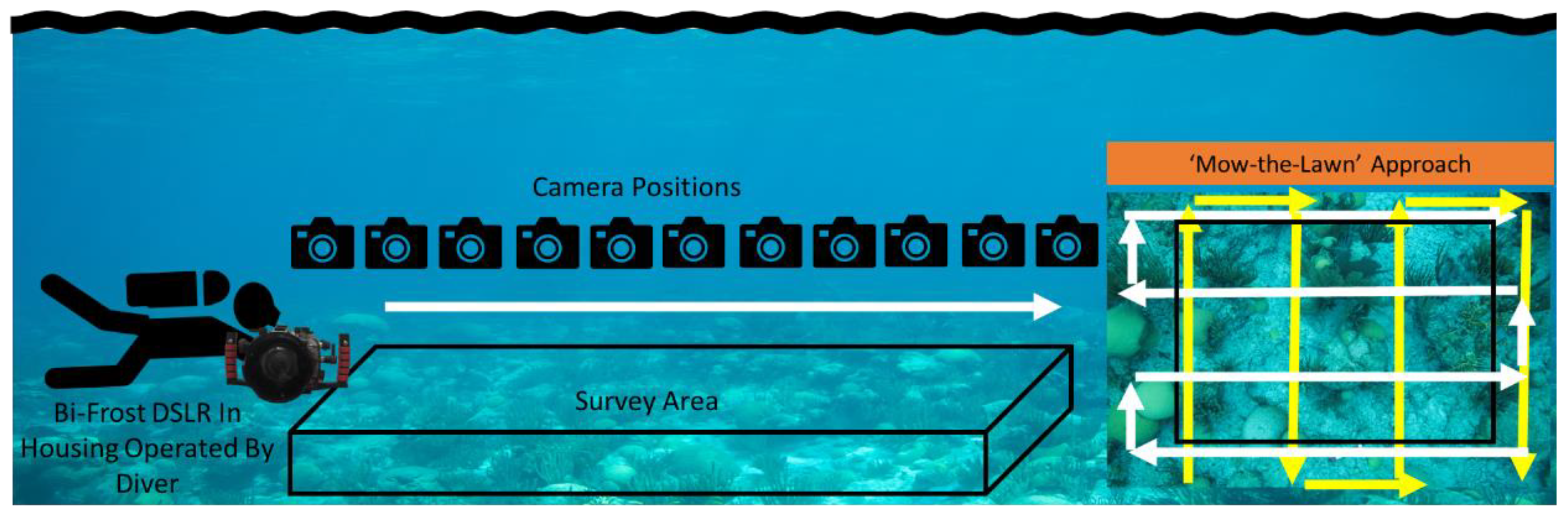
2.1. Hyperspectral Data Collection

Hyperspectral images were collected using the Bi-Frost DSLR hyperspectral camera, mounted in a waterproof case (Ikelite, Indianapolis, IN, USA) carried by a diver. The hyperspectral imager uses a similar method to push-broom imaging to generate 3D data from a 2D imager whereby the camera is scanned; in this instance, the method is known as “windowing”. These imagers obtain data by scanning across the scene in one dimension [Y], but in so doing, it is acquiring a 2D image [X, λ] in a single frame [26]. The pass band on the filter is a function of its position on the filter.

To enable full spectral information of the survey area to be generated, the camera was required to start and finish imaging one full frame before and after the survey area. This ensures that every part of the LVF has covered the target area so that there is a complete spectral reconstruction at each band. For maximum coverage, two “mow the lawn” or raster scan pattern surveys were used, one vertically across the site and one horizontally, as depicted in Figure 1. The individual transects were identical, with the second rotated and adjusted to account for the field of view of the camera. To record the image data, the DSLR was operated in video mode to capture the upper limit of the camera’s frame rate (30 fps); this allows for the option to bin or subsample the images in processing to balance the size and resolution required.

Images from the Bi-Frost DSLR were converted into hypercubes using a bespoke software solution developed at the University of Bristol. The resulting hypercube is comprised of 192 wavebands ranging from 339 nm to 789 nm at a resolution of 18 nm at band 450 nm. Hypercubes were then loaded into hyperspectral data software, ENVI (Harris Geospatial, Boulder, CO, USA), for analysis. The region of interest (ROI) tool was used to generate an average spectrum across a user-defined area of individual coral colonies within the hypercube; these were then used in the corrections outlined below. The coral colonies were arbitrarily selected to highlight an array of examples of the primary coral species present in Bermudan reefs.

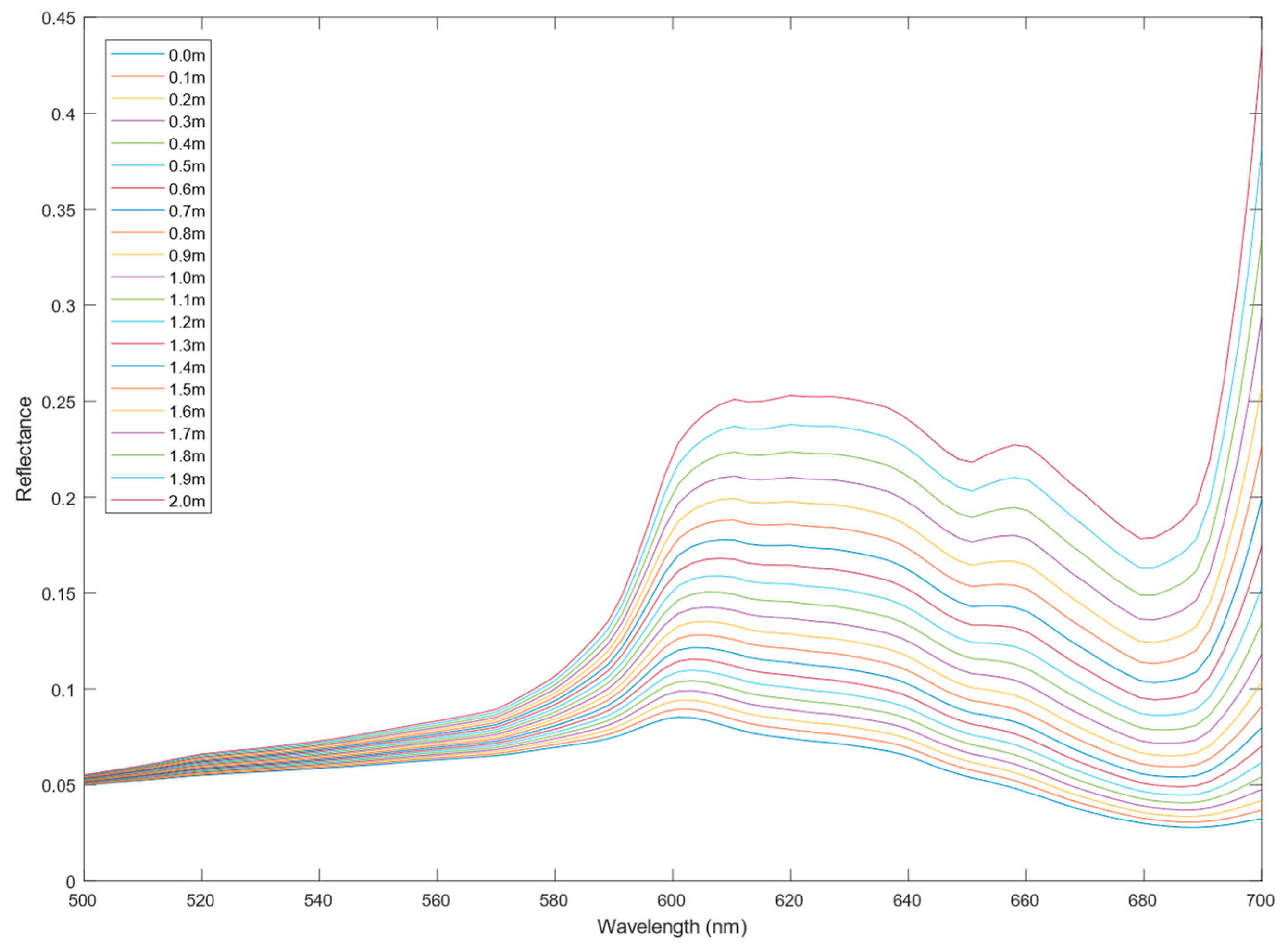
2.2. Hyperspectral Data Correction

The two-flow shallow water reflectance model (Equation (1), [27]) was used to correct the hyperspectral data for radiative transfer effects. R(Z,H) is the reflectance at depth Z in the water column (i.e., the imager) over a seafloor at depth H (i.e., the reef). R(Z,H) represents the image as collected by the Bi-Frost DSLR. R∞ is the reflectance, just below the sea surface, of an infinitely deep ocean. A is bottom albedo, and finally, exp[−2K(H − Z)] accounts for the exponential attenuation of reflectance between depths Z and H. Equation (1) shows that the reflectance of a water column is equal to the reflectance of the same water body in the absence of a bottom (R∞), plus the contrast between the bottom albedo and the reflectance of the body of water denoted by (A − R∞), which can be a positive or negative value, that is altered by attenuation through the water column. R∞ can be expanded, as shown in Equation (2), into backscatter (b_b) over 2K.

$$R\left(Z,H\right)=R\infty +\left(A-R\infty \right)exp[-2K\left(H-Z\right)]$$

(1)

$$R\infty =\frac{b_b}{2K}$$

(2)

In order to apply Equation (1), the values for the diffuse attenuation coefficient (K) and diffuse backscatter coefficient (b_b) need to be derived. The attenuation coefficient of water (K) is well established [28,29], and values have been obtained for a variety of water types and turbidities [12]. The backscatter (b_b) of water is also well established [28]. However, it is their values at the time and place of image collection that are required for the application of Equation (1). Both parameters can also be obtained in situ using a variable depth target calibrator (VDTC), which consists of five white reference targets set at different heights on a PVC pipe structure. Given the known height of each target, values for K and b_b can be derived via nonlinear regression. Approximations of H − Z can be obtained from the recorded depth of the diver and from structure-from-motion reconstructions, as outlined below, but as discussed in Section 3, more robust mechanisms are required to properly apply corrections. With all these variables parameterized, Equation (1) can be inverted to analytically solve for A, the bottom reflectance.

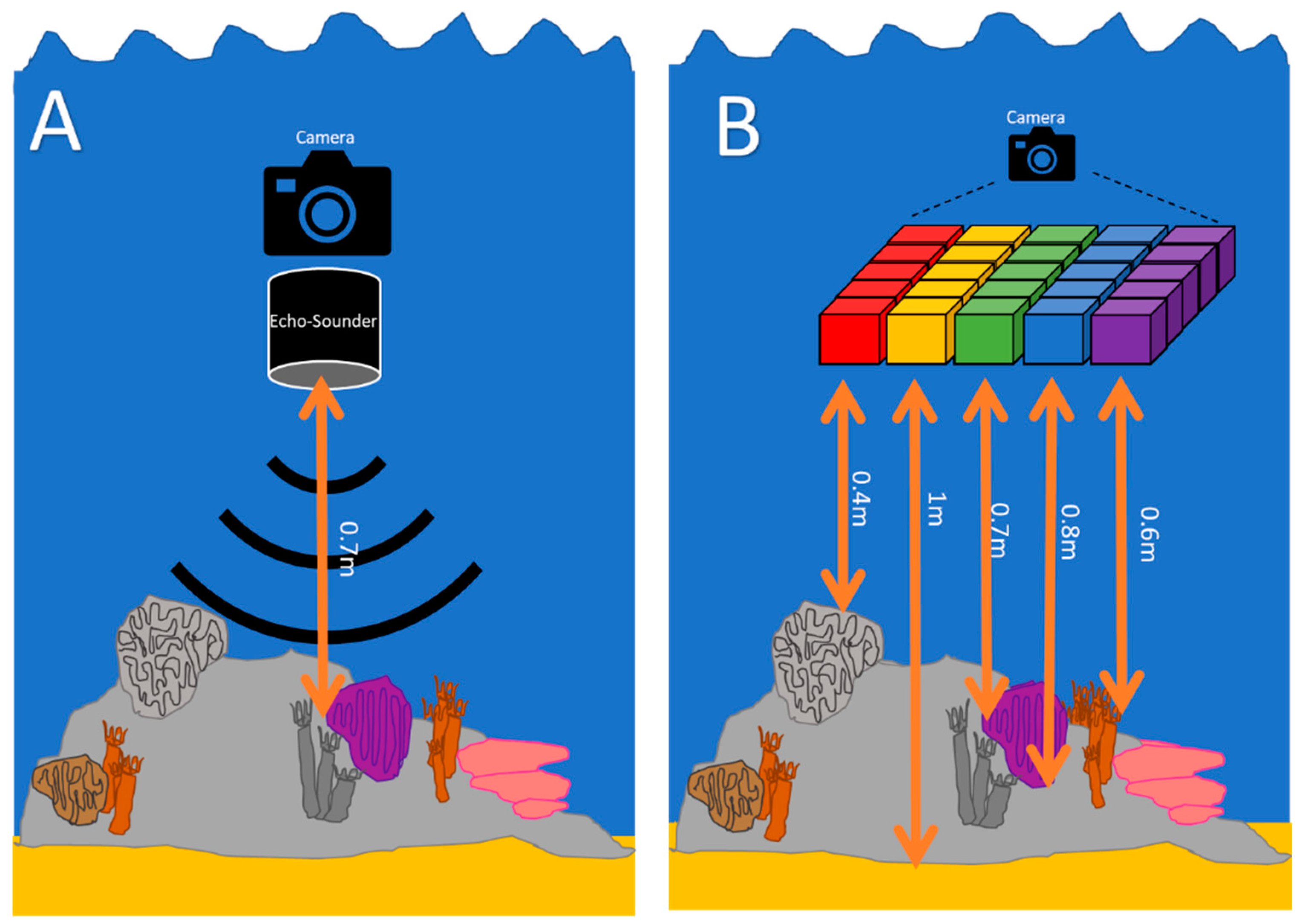
2.3. Strucutre-from-Motion (SfM) Photogrammetry

Due to the overlaps required for hyperspectral imaging, the images produced from the camera are also ideal for use in photogrammetry software. Raw images gathered from the imager were processed in Metashape (v1.7, Agisoft, St. Petersburg, Russia) to generate digital elevation models, as outlined in [12,30]. This technique also creates a composite image of all the stitched photo data, known as a photomosaic, which can be used for the identification and zonation of reefs. However, crucially, colour information is not present in these images due to the filtering of the Bi-Frost DSLR, and as such, the images are in grey scale, as is any resulting photomosaic. The technique also maps camera positions, i.e., where each image is relative to the whole scene; these can be used to gather approximations of the distance between the position of the imager and the scene (reef), allowing for approximations of H − Z.

2.4. Spectral Classification

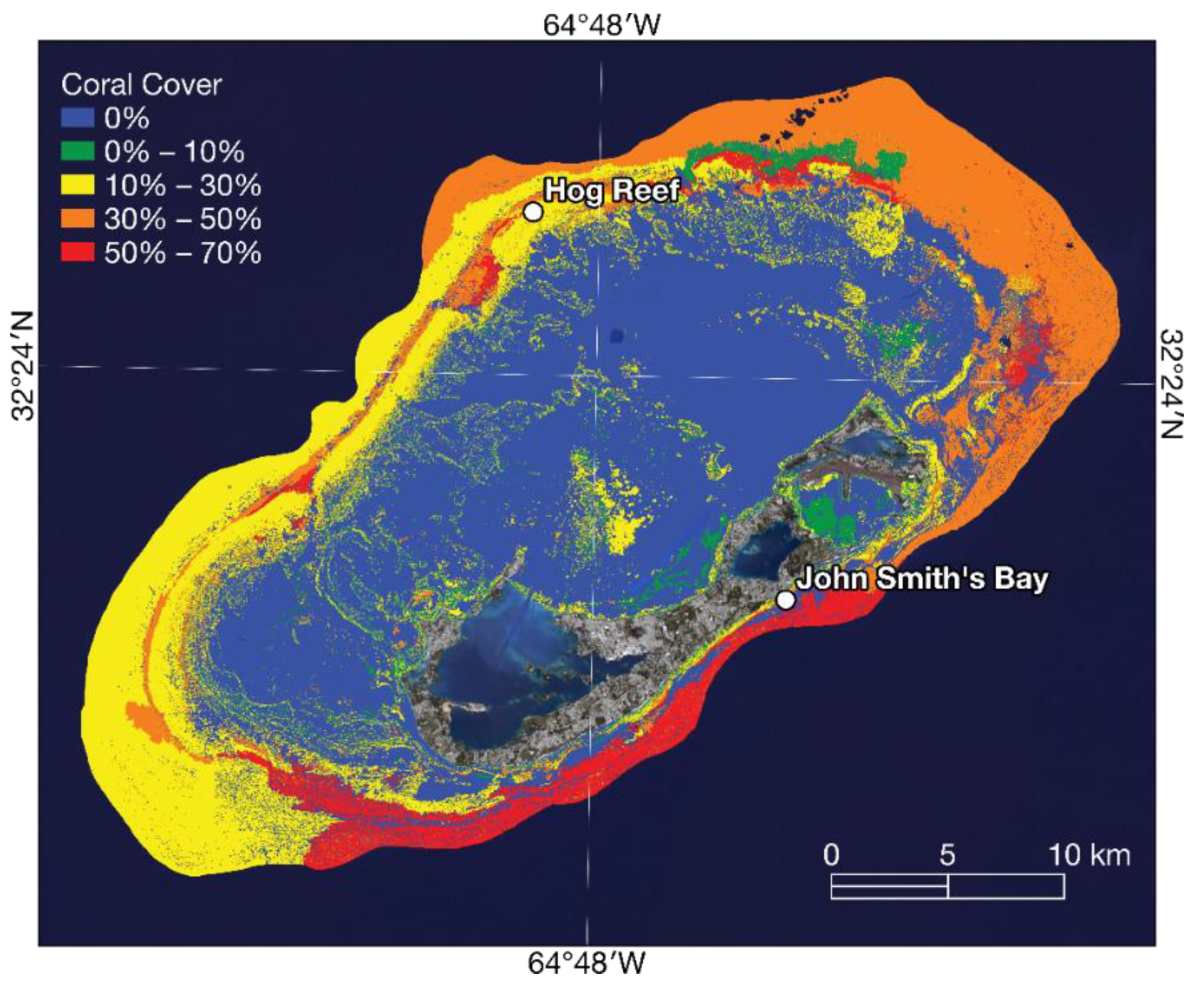
To gather data on benthic habitat coverage, automatic spectral classification was used in ENVI (Harris geospatial solutions, Version 5.5).

Spectral classification was conducted using training data in the form of three ROIs created from areas of basic benthic habitat type, such as substate (sand/rock), hard coral, and soft coral, as previously defined by Hochberg, 2000 [31]. An additional two reference ROIs were used to classify the void, areas outside of the reconstruction, and the white reference target. The algorithm used for classification was a minimum distance classifier, which uses the mean of each ROI class and calculates the Euclidean distance from each unknown pixel to each class. The pixels are then assigned an ROI class based on the nearest class, with no thresholding. During the classification process the data was smoothed by applying a kernel size of 3, which removes speckling noise, and a minimum aggregate size of 9 to remove small regions of less than 9 pixels.

2.5. Survey Area

To demonstrate the capabilities of the imaging system, small sections of a shallow reef (<15 m) were imaged at a distance of 3–4 m. Using the camera’s field of view and defined distances for the survey area, it is possible to plan other parameters of the survey, such as diver swimming speed. This was calculated assuming that a diver moving 0.51 m per second, or 1 knot, would yield a frame-to-frame overlap of 99.02%. For traditional photogrammetry surveys, the overlap required for “good” reconstruction is typically around 60–80% [32]. However, for this method, higher overlap increases the number of points used in each wavelength band, thus increasing the resolution of the resulting hypercubes. For multiple line transects, a standard sidelap of 40% [32] is adequate, as for these surveys, each transect was required to be spaced 0.95 m from the next. The depths of the survey were measured using the diver’s dive computer (Zoop, Suunto, Vantaa, Finland) and pressure gauge to determine the average depth of the reef, as well as the depth of the diver.

The study areas in Bermuda were Hog Reef (64°49′48.36″ W, 32°27′47.23″ N) and John Smith’s Bay (64°42′43.05″ W, 32°18′51.38″ N), as shown in Figure 2. These reefs were selected mainly due to their accessibility and to coincide with other ongoing field research at the Bermuda Institute of Ocean Sciences. Hog Reef lies on Bermuda’s northern rim reef and has a lower coral cover ≈ 10–30%. John Smith’s Bay has a fringing reef, with a high coral cover ≈ 50–70% [33]. The selection of these study areas allows for a comparative analysis between reefs with varying coral cover and reef types. Reefs with higher coral cover, such as John Smith’s Bay, enable the imaging system to capture a greater number of points of interest. The higher density of the coral colonies and associated structures in these areas provides more distinct features for matching and alignment in the image stitching process. This increased number of points improves the accuracy and precision of the final stitched images, enhancing the overall quality of the data captured. On the other hand, reefs with a lower coral cover, like Hog Reef, present a different testing scenario. In these areas, fewer coral colonies and their associated structures reduce the number of distinct points of interest and unique features available for imaging alignment and matching by the stitching software.

3. Results

3.1. RGB Represetations of Hyperspectral Data

Since hyperspectral data is inherently three-dimensional, the following Figure 3 and Figure 4 present two-dimensional projections of the hyperspectral data. To achieve this, the data is displayed as an RGB image using user-defined bands, specifically red (640 nm), green (549 nm), and blue (471 nm). It is important to note that these datasets comprise 192 individual reconstructions at each wavelength band, captured by the linear variable filter (LVF). As a result, when overlaying the data, minor alignment errors may occur. Additionally, incomplete spectral data can be observed along the edges and ends of the dataset, indicating a lack of complete spectral information across the entire spectral range.

The lower section of the images highlights the regions of interest, which correspond to specific coral colonies. By selecting all the points in the three-dimensional data within these regions, an averaging process is performed, generating a single representative spectrum. This approach allows for a more comprehensive analysis by capturing the overall characteristics and properties of the coral colonies in question.

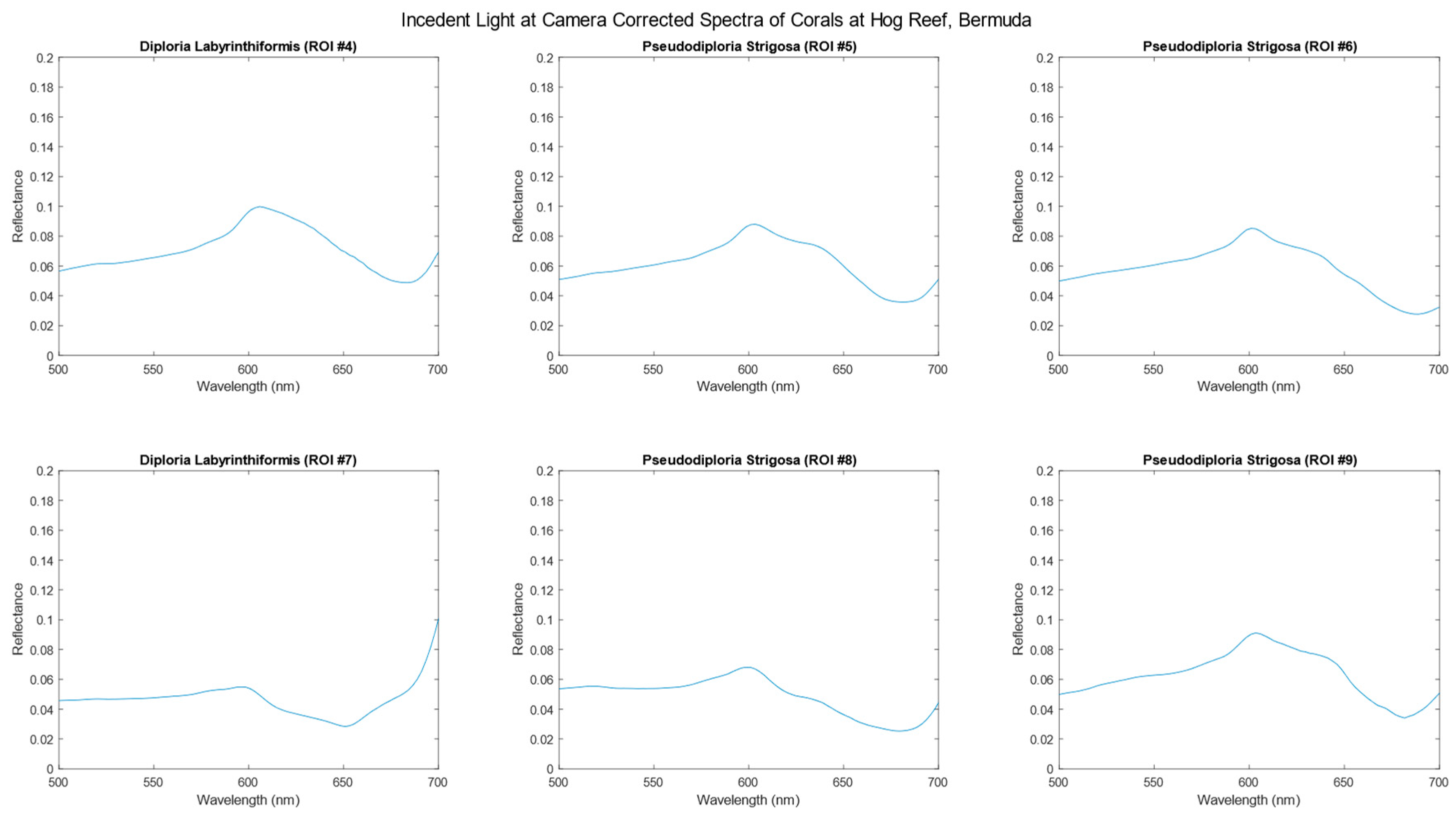
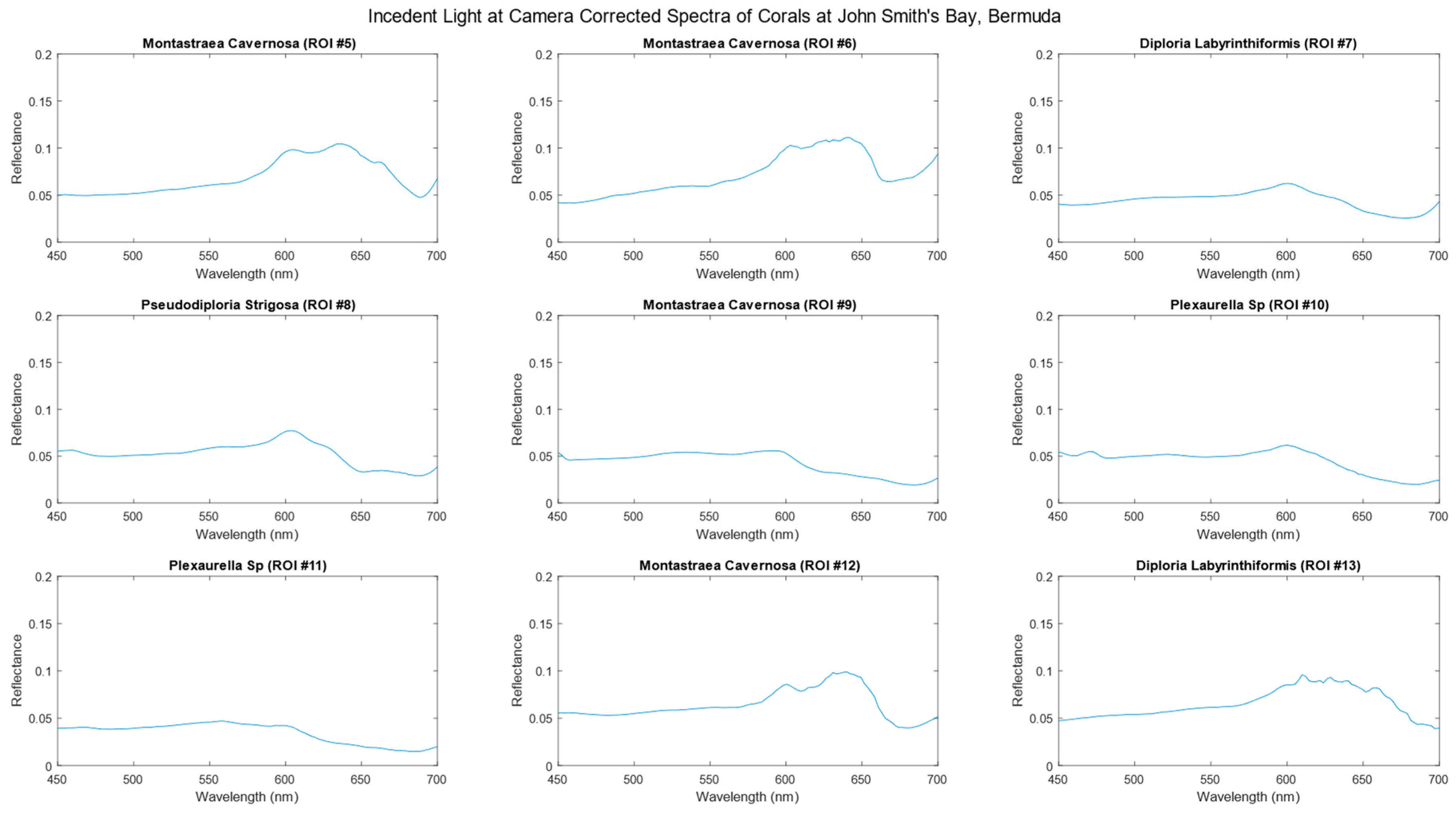
3.2. Incident Light Corrected Hyperspectral Data

Figure 5 and Figure 6 depict the average spectra of each region of interest (ROI) that have been corrected to account for the incident light, resulting in reflectance units. As evident in the data, the characteristic trough between 650 and 600 nm represents the absorption profile of chlorophyll. The ROIs represent a selection of common coral species found in Bermudan waters.

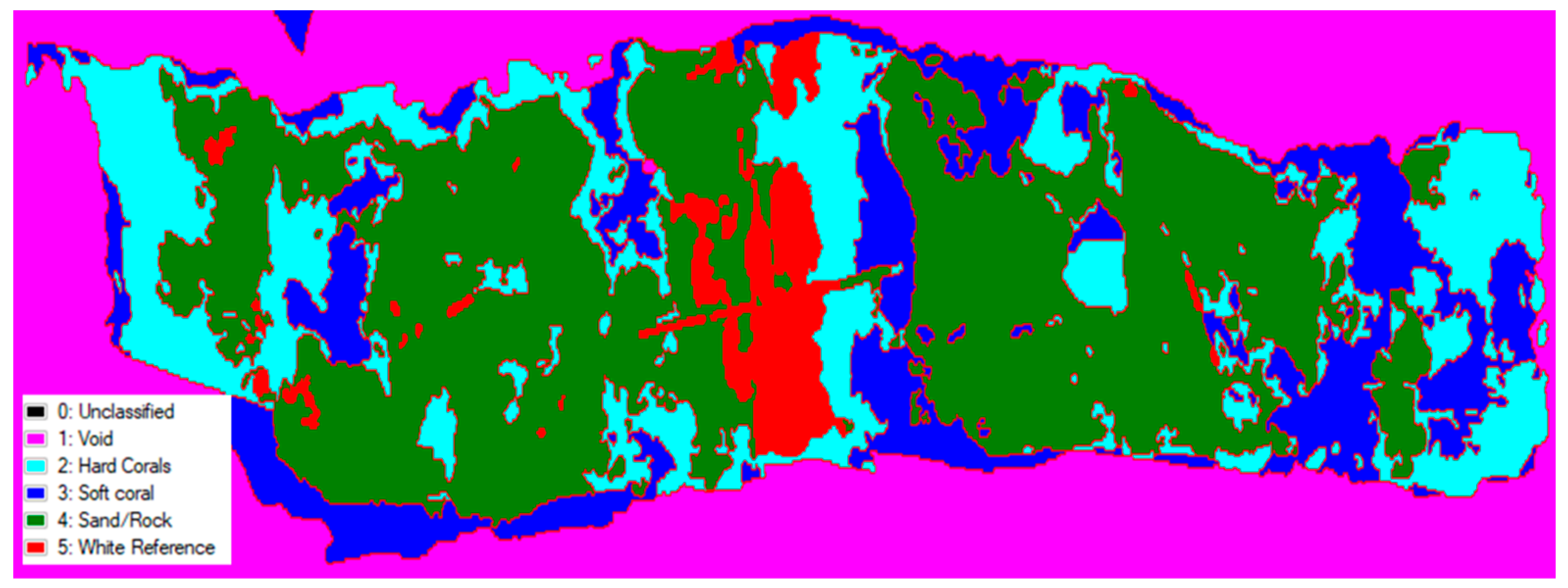
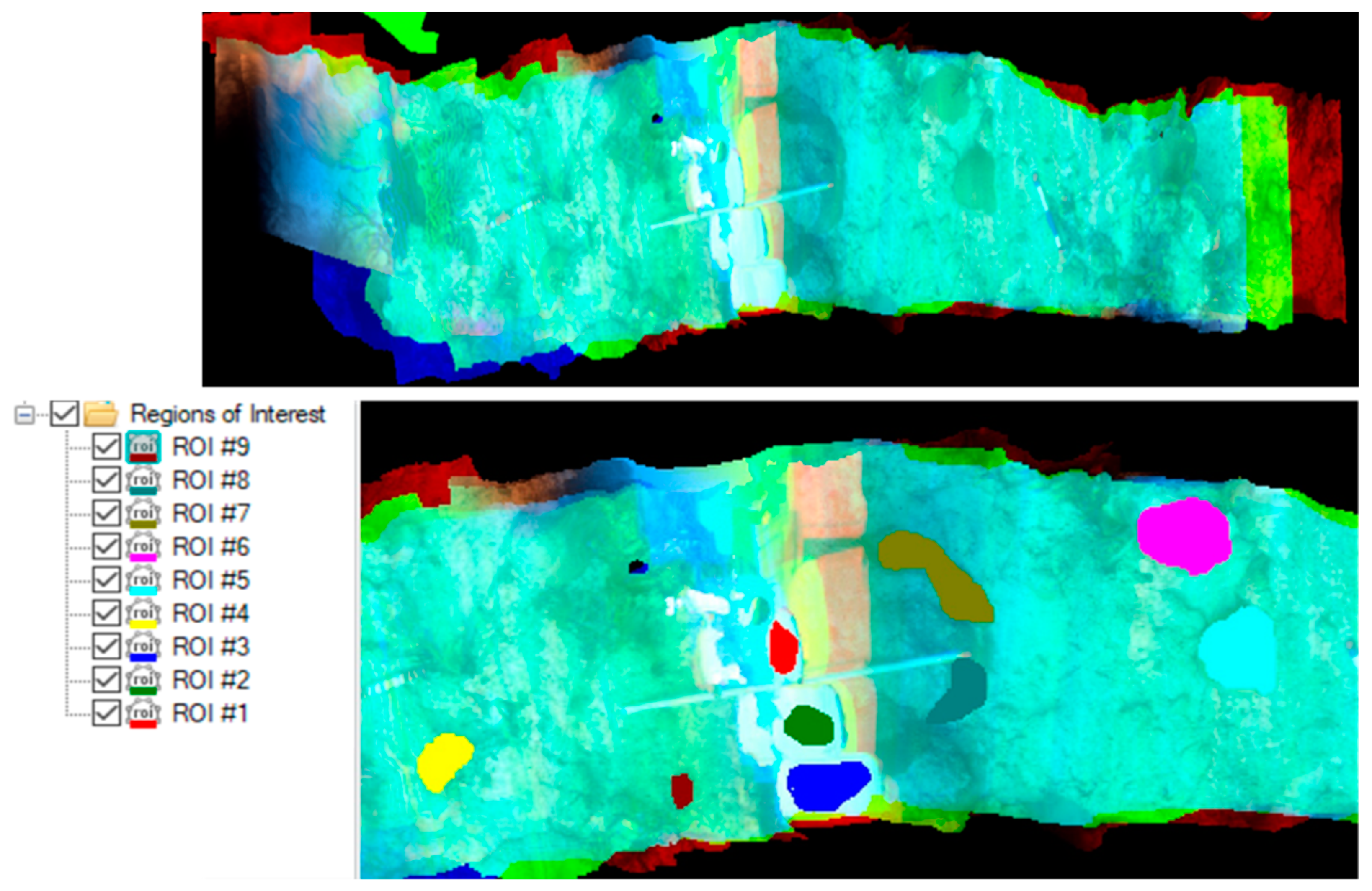
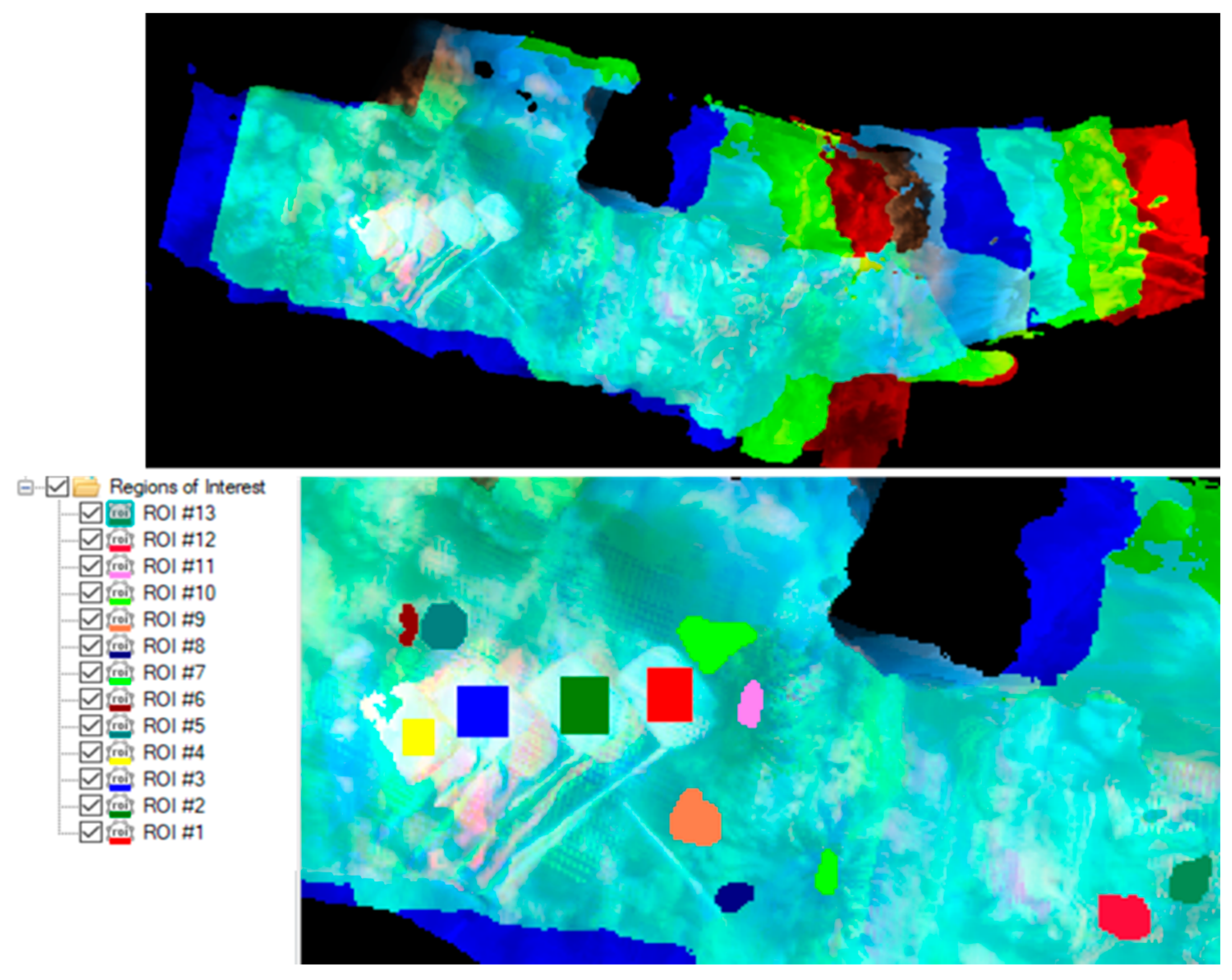
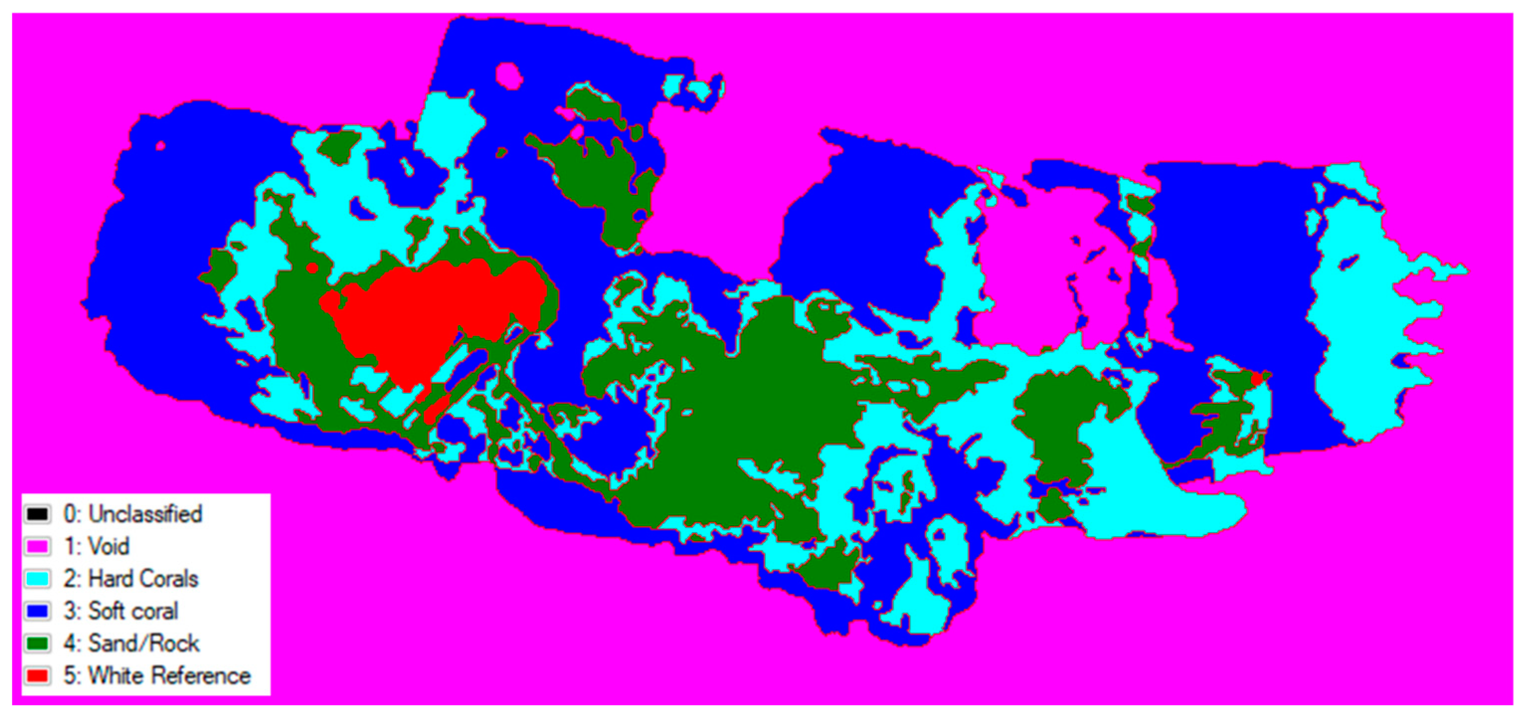
3.3. Simple Spectral Classification

Using spectral classification, i.e., the automatic grouping of pixels within the hypercube based on spectral similarities. Figure 7 and Figure 8 show the simple spectral classification of each reef using spectral data gathered from ROIs of a selection of benthic types: hard corals, soft corals, sand/rock, and the white reference.

Table 1. Percentage coverage of types of benthos at Hog Reef, Bermuda, based on ENVI classification shown in Figure 8.

Class	Pixel Count	Percentage Coverage (%)
Hard Coral	30,358	25.437
Soft Coral	25,258	21.248
Sand/Rock	57,513	48.190
White Reference	6116	5.125

and

Table 2. Percentage coverage of types of benthos at John Smith Reef, Bermuda, based on ENVI classification shown in Figure 8.

Class	Pixel Count	Percentage Coverage (%)
Hard Coral	46,875	30.179
Soft Coral	81,835	52.689
Sand/Rock	22,951	14.777
White Reference	3657	2.355

, show the percentage cover of these benthic types for both reefs.

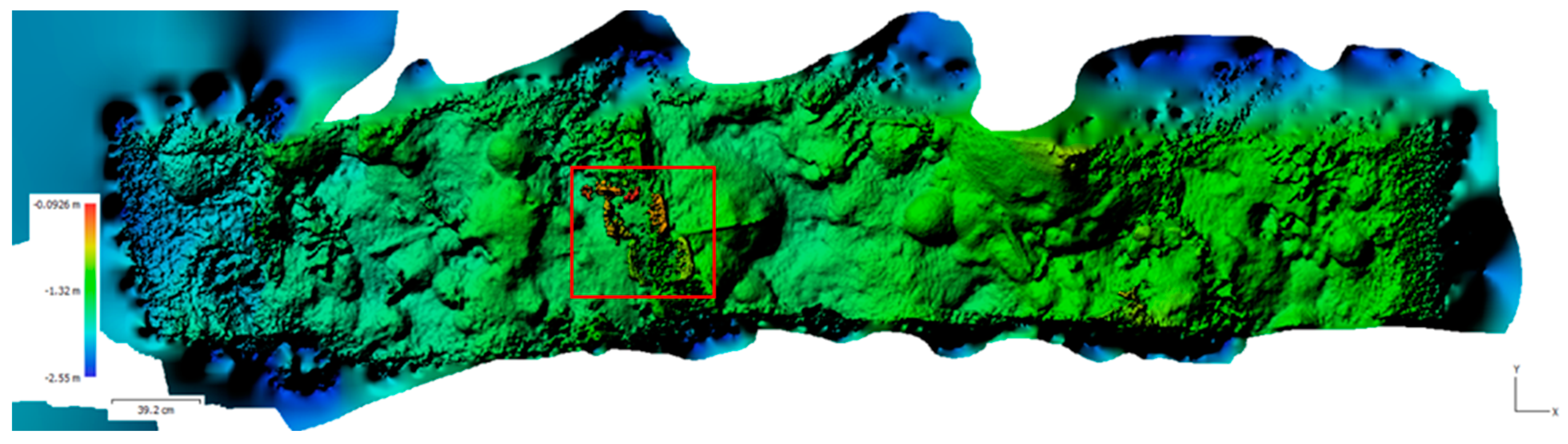
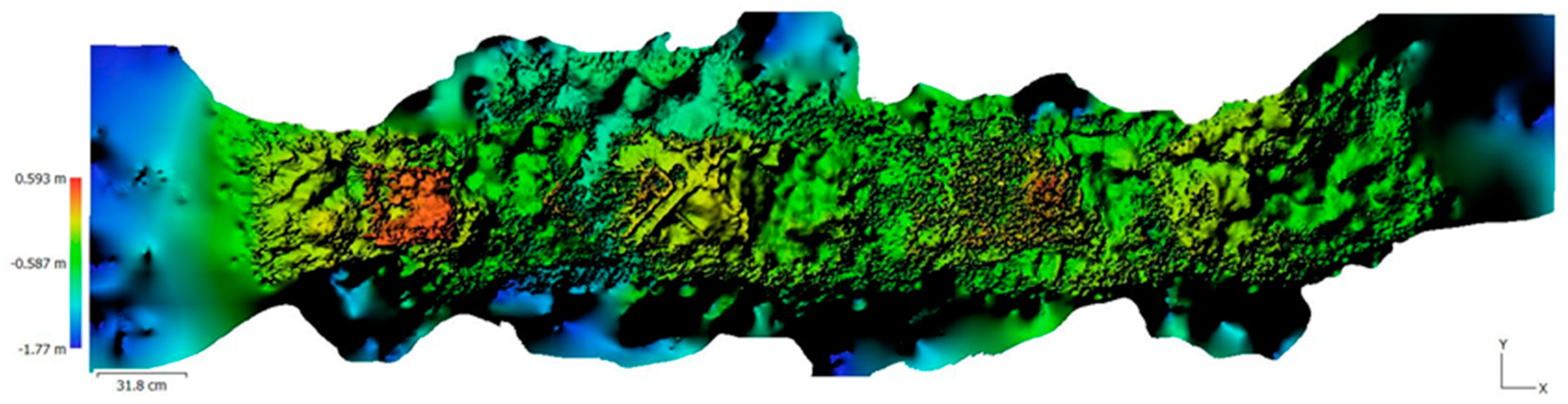
3.4. Digital Elevation Models (DEM) of Reefs from Images Taken by a Hypersepctral Imager

The presented Figure 9 and Figure 10 showcase the digital elevation models generated by Agisoft Metashape using image data captured by the Bi-Frost hyperspectral imager. Due to the images being stitched by different software, they differ slightly to the hypercube reconstructions made using the same images. The color representation within the figures serves to highlight the variation in height, emphasizing the three-dimensional nature of the data. By assigning different colors to distinct height levels, the figures provide a visual representation of the topographical characteristics of the captured scene.

3.5. Physical Information of the ROIs Derived from DEMs

Table 3. Perimeters and areas of the regions of interest (ROIs) associated with corals at Hog Reef derived from the digital elevation model (DEM) shown in Figure 4.

Label	Species	Perimeter (cm)	Area (cm2)
ROI #4	DLAB	52.66	1.53
ROI #5	PSTR	75.33	3.75
ROI #6	PSTR	74.83	3.70
ROI #7	DLAB	83.13	2.53
ROI #8	PSTR	61.63	2.36
ROI #9	PSTR	23.22	0.35

DLAB: Diploria labyrinthiformis; PSTR: Pseudodiploria strigosa.

and

Table 4. Perimeters and areas of the regions of interest (ROIs) associated with corals at John Smith’s Bay derived from the digital elevation model (DEM) shown in Figure 5.

Label	Species	Perimeter (cm)	Area (cm2)
ROI #5	MCAV	20.81	0.32
ROI #6	MCAV	17.25	0.20
ROI #7	DLAB	23.84	0.32
ROI #8	PSTR	12.40	0.11
ROI #9	MCAV	17.97	0.22
ROI #12	MCAV	17.04	0.21
ROI #13	DLAB	30.30	0.63

MCAV: Montastraea cavernosa; DLAB: Diploria labyrinthiformis; PSTR: Pseudodiploria strigosa.

show the extracted physical information derived from the DEM data of the same ROIs used in the spectral data analysis. These tables highlight the diverse range of data that can be extracted from the DEM, including measurements such as perimeter and area.

4. Discussion

Due to the Bi-Frost DSLR being a modified camera, we are able to run the raw images through traditional SfM photogrammetry processes to generate a digital elevation model (DEM) for each scene (Figure 8 and Figure 9). Most commercial grade hyperspectral imagers do not offer this as an option, as they often do not capture data in the same way. The only drawback to using images captured by the Bi-Frost DSLR for this purpose is that due to the LVF, the individual images are greyscale and have a gradient across them which represents the differing amount of light present at each of the wavebands positioned across the sensor. This means that the outputs from the photogrammetry models may not be suitable for tasks involving the photomosaic, such as identification, but they do contain all the relevant information for DEMs.

To demonstrate an application of DEM data, the coral ROIs previously isolated for spectral data were utilized to provide surface area measurements (Table 3 and Table 4). These measurements can be used to determine important factors such as topography, rugosity, and surface area of the reef. The use of these topographic measurements is limited by the photogrammetry software’s ability to reconstruct the 3D information of objects. Thick, static objects are the easiest to reconstruct, as they have many reference points that can be used for alignment. In contrast, thin objects tend to have fewer reference points due to their reduced surface areas. The reconstruction of the white reference tower in Figure 9 (marked by a red square) illustrates this problem: the 2 mm thick targets have only been partially reconstructed. This photogrammetric technique is also unable to reconstruct dynamic objects, such as soft corals and fish, because they change position and shape between image frames. This causes the reference points to change drastically, and matching these objects from one image to the next is often not possible. Another potential drawback of using this technique for assessments of surface area measurements is that corals with complex morphologies, such as arborescent and corymbose corals (branching corals) will be under reconstructed. Due to their complex structure and the limitations of the current image reconstruction software, any top-down only measurements will need to be complemented with additional angles to provide more complete measures of the 3D structure. However, this is very time consuming on a reef scale. Conversely, the technique works well for measures of more simple coral morphologies, such as massive corals, as presented in this study.

The spectral data in Section 3.2 represents the signal measured by the camera converted into units of reflectance. This was achieved by blocking the field of view (FOV) of the camera using a white PTFE slate, considered to have 100% reflectance, to capture the incident light present at the camera before each survey. This incident light correction demonstrates that reflectance data can be captured in situ by low-cost hyperspectral imagers. However, in order for these datasets to be utilised in ecological monitoring, the spectral signal at the imaged object needs to be obtained. The primary issue faced by LVF-based imagers is that due to the attenuation of light in water, the amount of light available across all the bands in the sensor means that the camera’s wavelength range is reduced, and thus, the amount of the usable image required for stitching is reduced. As a result, both the final wavelength range and the stitching software’s ability to match images to one another are hindered.

As discussed in Section 2.2, to fully correct the data, the two-flow shallow water reflectance model (Equation (1), [27]) must be applied. Given that both K and b_b are per unit depths, the depth is an important consideration, especially for morphometrically complex environments such as reefs. Therefore, having an accurate depth measurement is vital to generating the ‘true’ spectra of the object being imaged. To highlight this issue, ROI #6 from John Smith’s Bay was corrected using Equation (1) and values from the literature in [28,29] for k and b_b, where the depth was adjusted every 0.1 m, as shown in Figure 11. This highlights that the depth measurement should be as accurate as possible, as even a 10 cm difference can have a significant impact on the spectra.

The primary aim of this experiment was to show that hyperspectral data could be generated by low-cost hyperspectral imagers for underwater environments, as the challenges with image stitching and imaging underwater are difficult. As a result of this, the true depths of the ROIs are not known, and we cannot accurately compare our spectra to known values. However, the data could still be used to perform a simple automatic classification using ENVI’s spectral classification tool to demonstrate how the data can be utilised. Using ROI “training” data from areas of different benthic types, such as hard coral, soft coral, and sand/rock, in the hypercube, an automatic classification was performed (Figure 7 and Figure 8). The classification assigns a likelihood, based on user defined parameters, of how similar each pixels spectra is to those of the reference groups and assigns it to a specific group, depicted by a colour in this example. This data can then be used to determine the percentage cover of each of the benthic groups used (Table 1 and Table 2), thus giving researchers a method to quickly assess coral cover and the change in the distribution of benthic types. As shown by the data, this is not a perfect solution, as some small areas are clearly misidentified, i.e., the white reference, which has been identified in several areas outside of where the targets were situated. The data presented in this study highlights that for accurate assignment, the spectral classification requires sufficient training or reference data. The more data available to it the more accurate the classification will be; therefore, more accurate the spectral data in turn leads to more accurate classifications.

Through this study, valuable insights have been gained that can inform future improvements to the imaging device, particularly in achieving more accurate depth measurements. One simple potential enhancement is the incorporation of a range finding system, such as an echosounder or range finding LIDAR, incorporated into the system. This addition would enable each captured image to be associated with a corresponding depth measurement, providing depth information for each individual image (as shown in Figure 12A), accounting for any changes in distance from the reef to the imager, such as changes in the buoyancy of the diver. It is important to note that while a range finding system could provide depth measurements per image, its applicability may be limited to environments with relatively low complexity and rugosity. In such environments, where objects within the image exhibit minimal height variations, depth measurements from a range finding system could yield reasonably accurate results.

However, to address the complexities associated with depth measurements in more diverse environments, a more comprehensive solution is needed. One such solution involves generating distance information from each pixel to the object, accounting for both angle and distance (depicted graphically in Figure 12B). This could be achieved using advanced stitching software, such as SfM photogrammetry, and combining it with the hypercube reconstruction. By using the point cloud information generated in the SfM workflow, we can derive each pixel’s location, its waveband, and the distance from each pixel to the point cloud. Using the distance information, as provided by the point cloud, allows the algorithm to be written to automatically apply the attenuation coefficient to each pixel individually. This would lead to extremely accurate hyperspectral data in UHI applications and allow for the generation of 4D [x, y (image), λ (wavelength), Z (height)] data. However, it is important to consider the computational requirements associated with this approach. The processing power necessary for generating the hyperspectral reconstruction as part of the photogrammetry process may necessitate the utilization of supercomputers and lead to very long processing times. However, these advancements would not only enhance the quality of the data collected but also enable the generation of comprehensive 4D representations of marine environments, providing valuable insights for various applications in research and monitoring.

As highlighted in the introduction, the application of UHI extends beyond this specific case study. Numerous other disciplines and fields can benefit from advances in UHI, and it is important to recognize that the challenges associated with UHI are not limited to a single application. Therefore, the proposed solutions discussed above hold relevance for all of these disciplines. By addressing the technical and financial limitations associated with UHI, the full potential of this technology can be unlocked, facilitating advancements across various scientific disciplines. The utilization of low-cost hyperspectral imagers constructed from off-the-shelf components and their capability to compensate for unstable movements are not only relevant to this marine applications, but also hold promise for a broad range of applications outside the marine environment.

The data presented in this study represent two small areas of reef, and additional work is required to gather data across larger sections. Scaling up the software used is of paramount importance to effectively handle these larger datasets, enabling the efficient processing and analysis of the acquired hyperspectral data. Furthermore, integrating pixel distances into the analysis pipeline to generate 4D hyperspectral data would offer invaluable insights for a range of HSI applications particularly in environmental contexts.

Building upon a successful demonstration of 4D hyperspectral data, the next step would be to conduct repeat surveys of reef areas over multiple time periods. This approach would enable the creation of a time-series dataset, which is essential for studying temporal changes and dynamics in reef health. By comparing data collected at different time points, change detection algorithms could be applied to track and quantify alterations in reef condition, such as coral bleaching events, changes in coral cover, damage from storm events, or shifts in biodiversity, over extended time periods. It is important to note that the spectral data gathered can be used to accurately and automatically classify broad benthic types (coral, algae, sand), as previously outlined by [31,34]. Due to the extensive coverage provided by hyperspectral data, further refinement of the classifications will develop rapidly with return surveys [35]. However, while identification of coral species by spectral data alone is currently not possible, in future, a combination of enhanced spectral libraries and the use of other complementary metrics, such as photomosaics and 3D information machine learning algorithms, may achieve this goal. The true strength of the technique is its allowance of non-invasive physiological assessments of organism health, which will help us understand how marine habitats are impacted by stressors such as heatwaves, and crucially, how they recover from such events. This will enable us to better understand the impacts and to identify pathways to mitigate and adapt.

In conclusion, the Bi-Frost DSLR was able to effectively process underwater data to generate hypercubes and extract spectral information from coral reefs. The successful implementation of the Bi-Frost imager represents a major milestone in the development of a low-cost, in situ marine hyperspectral imaging technique. By providing an affordable spectroscopy tool, the capacity to expand the current capabilities of marine scientists to understand and preserve marine ecosystems is increased. This affordability opens up extended opportunities for data collection across larger reef areas, enhancing our understanding of ecosystem dynamics and enabling comprehensive monitoring using spectroscopic techniques. This study is the first step in laying the groundwork for establishing the Bi-Frost imager’s use in coral reef monitoring. Future advancements will focus on improving the image processing algorithms to generate hyperspectral data, expanding the spectral range, and incorporating advanced data analysis techniques into standard surveyance. These developments will contribute to a robust and reliable marine hyperspectral imaging technique, aiding ongoing efforts to assess and monitor coral reef and marine ecosystem health.

References

1. Ødegård, Ø.; Mogstad, A.A.; Johnsen, G.; Sørensen, A.J.; Ludvigsen, M. Underwater hyperspectral imaging: A new tool for marine archaeology. Appl. Opt. 2018, 57, 3214–3223. [Google Scholar] [CrossRef] [PubMed]
2. Johnsen, G.; Ludvigsen, M.; Sørensen, A.; Aas, L.M.S. The use of underwater hyperspectral imaging deployed on remotely operated vehicles—Methods and applications. IFAC-Papers Online 2016, 49, 476–481. [Google Scholar] [CrossRef]
3. Mogstad, A.A.; Odegard, O.; Nornes, S.M.; Ludvigsen, M.; Johnsen, G.; Berge, J. Mapping the historical shipwreck Figaro in the high arctic using underwater sensor-carrying robots. Remote Sens. 2020, 12, 997. [Google Scholar] [CrossRef]
4. Beck, A.J.; Kaandrop, M.; Hamm, T.; Bogner, B.; Kossel, E.; Lenz, M.; Haeckel, M. Rapid shipboard measurement of net-collected marine microplastic polymer types using near-infrared hyperspectral imaging. Anal. Bioanal. Chem. 2023, 415, 2989–2998. [Google Scholar] [CrossRef] [PubMed]
5. Serranti, S.; Palmieri, R.; Bonifazi, G.; Cózar, A. Characterization of microplastic litter from oceans by an innovative approach based on hyperspectral imaging. Waste Manag. 2018, 76, 117–125. [Google Scholar] [CrossRef]
6. Freitas, S.; Silva, H.; Silva, E. Hyperspectral Imaging Zero-Shot Learning for Remote Marine Litter Detection and Classification. Remote Sens. 2022, 14, 5516. [Google Scholar] [CrossRef]
7. Balsi, M.; Esposito, S.; Moroni, M. Hyperspectral characterization of marine plastic litters. MetroSea 2019, 2, 28–32. [Google Scholar] [CrossRef]
8. Garaba, S.P.; Dierssen, H.M. An airborne remote sensing case study of synthetic hydrocarbon detection using short wave infrared absorption features identified from marine-harvested macro- and microplastics. Remote Sens. Environ. 2018, 205, 224–235. [Google Scholar] [CrossRef]
9. Teague, J.; Megson-Smith, D.A.; Yannick, V.; Scott, T.B.; Day, J.C.C. Underwater Spectroscopic Techniques for In-Situ Nuclear Waste Characterisation; Waste Management: Phoenix, AZ, USA, 2022; pp. 1–9. [Google Scholar]
10. Chennu, A.; Färber, P.; De’ath, G.; De Beer, D.; Fabricius, K.E. A diver-operated hyperspectral imaging and topographic surveying system for automated mapping of benthic habitats. Sci. Rep. 2017, 7, 7122. [Google Scholar] [CrossRef]
11. Johnsen, G.; Volent, Z.; Dierssen, H.; Pettersen, R.; Van Ardelan, M.; Søreide, F.; Moline, M. Underwater hyperspectral imagery to create biogeochemical maps of seafloor properties. Subsea Opt. Imaging 2013, 508, 536e–540e. [Google Scholar]
12. Teague, J.; Megson-Smith, D.A.; Allen, M.J.; Day, J.C.C.; Scott, T.B. A Review of Current and New Optical Techniques for Coral Monitoring. Oceans 2022, 3, 30–45. [Google Scholar] [CrossRef]
13. Gleason, A.C.R.; Reid, R.P.; Voss, K.J. Automated Classification of Underwater Multispectral Imagery for Coral Reef Monitoring. In Proceedings of the OCEANS 2007 Conference, Vancouver, BC, Canada, 29 September–4 October 2007. [Google Scholar] [CrossRef]
14. Thompson, D.R.; Hochberg, E.J.; Asner, G.P.; Green, R.O.; Knapp, D.E.; Gao, B.C.; Garcia, R.; Gierach, M.; Lee, Z.; Maritorena, S.; et al. Airborne mapping of benthic reflectance spectra with Bayesian linear mixtures. Remote Sens. Environ. 2017, 200, 18–30. [Google Scholar] [CrossRef]
15. Teague, J.; Willans, J.; Allen, M.; Scott, T.; Day, J. Hyperspectral imaging as a tool for assessing coral health utilising natural fluorescence. J. Spectr. Imaging 2019, 8, a7. [Google Scholar] [CrossRef]
16. Kok, J.; Bainbridge, S.; Olsen, M.; Rigby, P. Towards Effective Aerial Drone-based Hyperspectral Remote Sensing of Coral Reefs. In Proceedings of the Oceans 2020 Conference, Biloxi, MS, USA, 5–30 October 2020. [Google Scholar] [CrossRef]
17. Teague, J.; Willans, J.; Megson-Smith, D.A.; Day, J.C.C.; Allen, M.J.; Scott, T.B. Using Colour as a Marker for Coral ‘Health’: A Study on Hyperspectral Reflectance and Fluorescence Imaging of Thermally Induced Coral Bleaching. Oceans 2022, 3, 547–556. [Google Scholar] [CrossRef]
18. Joyce, K.E.; Phinn, S.R. Hyperspectral analysis of chlorophyll content and photosynthetic capacity of coral reef substrates. Limnol. Oceanogr. 2003, 48, 489–496. [Google Scholar] [CrossRef]
19. Hochberg, E.J.; Apprill, A.M.; Atkinson, M.J.; Bidigare, R.R. Bio-optical modeling of photosynthetic pigments in corals. Coral Reefs 2006, 25, 99–109. [Google Scholar] [CrossRef]
20. Boyd, J. Drones survey the great barrier reef: Aided by AI, hyperspectral cameras can distinguish bleached from unbleached coral—[News]. IEEE Spectr. 2019, 27, 7–9. [Google Scholar] [CrossRef]
21. Casella, E.; Collin, A.; Harris, D.; Ferse, S.; Bejarano, S.; Hench, J.L.; Rovere, A. Mapping coral reefs using consumer-grade drones and structure from motion photogrammetry techniques. Coral Reefs 2017, 36, 269–275. [Google Scholar] [CrossRef]
22. Palandro, D.; Andréfouët, S.; Muller-Karger, F.E.; Dustan, P.; Hu, C.; Hallock, P. Detection of changes in coral reef communities using Landsat-5 TM and Landsat-7 ETM+ data. Can. J. Remote Sens. 2003, 2, 201–209. [Google Scholar] [CrossRef]
23. Joyce, K.E.; Phinn, S.R.; Roelfsema, C.M.; Neil, D.T.; Dennison, W.C. Combining Landsat ETM+ and Reef Check classifications for mapping coral reefs: A critical assessment from the southern Great Barrier Reef, Australia. Coral Reefs 2004, 23, 21–25. [Google Scholar] [CrossRef]
24. Mizuochi, H.; Tsuchida, S.; Mizuyama, M.; Yamamoto, S.; Iwao, K. Multi-band bottom index: A novel approach for coastal environmental monitoring using hyperspectral data. Remote Sens. Appl. Soc. Environ. 2022, 27, 100797. [Google Scholar] [CrossRef]
25. Foo, S.A.; Asner, G.P. Scaling up coral reef restoration using remote sensing technology. Front. Mar. Sci. 2019, 3, 79. [Google Scholar] [CrossRef]
26. Boreman, G.D. Classification of imaging spectrometers for remote sensing applications. Opt. Eng. 2005, 44, 013602. [Google Scholar] [CrossRef]
27. Maritorena, S.; Morel, A.; Gentili, B. Diffuse reflectance of oceanic shallow waters: Influence of water depth and bottom albedo. Limnol. Oceanogr. 1994, 39, 1689–1703. [Google Scholar] [CrossRef]
28. Buiteveld, H.; Hakvoort, J.H.M.; Donze, M. Optical properties of pure water. Ocean Opt. XII 1994, 2258, 174–183. [Google Scholar] [CrossRef]
29. Baker, K.S.; Smith, R.C. Optical properties of the clearest natural waters (200–800 nm). Appl. Opt. 1981, 20, 177–184. [Google Scholar] [CrossRef]
30. Teague, J.; Scott, T.B. Underwater Photogrammetry and 3D Reconstruction of Submerged Objects in Shallow Environments by ROV and Underwater GPS. J. Mar. Sci. Res. Technol. 2017, 1, 7. [Google Scholar]
31. Hochberg, E.J.; Atkinson, M.J. Spectral discrimination of coral reef benthic communities. Coral Reefs 2000, 19, 164–171. [Google Scholar] [CrossRef]
32. Colomina, I.; Molina, P. Unmanned aerial systems for photogrammetry and remote sensing: A review. ISPRS J. Photogramm. Remote Sens. 2014, 92, 79–97. [Google Scholar] [CrossRef]
33. Hochberg, E.J. Bermuda Benthic Community Mapping Program Report; Bermuda Department of Environment and Natural ReSources: Paget, Bermuda, 2015.
34. Hochberg, E.J.; Atkinson, M.J.; Apprill, A.; Andréfouët, S. Spectral reflectance of coral. Coral Reefs 2004, 23, 84–95. [Google Scholar] [CrossRef]
35. Zeng, K.; Xu, Z.; Yang, Y.; Liu, Y.; Zhao, H.; Zhang, Y.; Xie, B.; Zhou, W.; Li, C.; Cao, W. In situ hyperspectral characteristics and the discriminative ability of remote sensing to coral species in the South China Sea. Ocean. Opt. XII 2022, 59, 272–294. [Google Scholar] [CrossRef]
Figure 1. The Bi-Frost DSLR was operated by a diver following a “mow-the-lawn” survey pattern. The diver begins imaging before the start of the survey area to ensure that full spectral data is recorded to generate complete reconstructions. (Figure adapted from [12].)
Oceans 04 00020 g001
Figure 2. A map to show the reef locations in Bermuda, along with the percentage of coral cover using data from [33].
Oceans 04 00020 g002
Figure 3. Hyperspectral data of Hog Reef presented in red 640 nm, green 549 nm, and blue 471 nm user-defined bands (top). Hyperspectral data with the regions of interest highlighted and labeled are listed to the left of the bottom image.
Oceans 04 00020 g003
Figure 4. Hyperspectral data of John Smith’s Bay presented in red 640 nm, green 549 nm, and blue 471 nm user defined bands (Top). Hyperspectral data with the regions of interest highlighted and labeled are listed to the left of the bottom image.
Oceans 04 00020 g004
Figure 5. Hyperspectral data of corals, corrected for incident light occurring at the camera, highlighted as ROIs in Figure 2 at Hog Reef, Bermuda.
Oceans 04 00020 g005
Figure 6. Hyperspectral data of corals, corrected for incident light at the camera, highlighted as ROIs in Figure 3 at John Smith’s, Bermuda.
Oceans 04 00020 g006
Figure 7. Simple spectral classification of hyperspectral data at Hog Reef, Bermuda, into three habitat classes (hard corals, soft corals, sand/rock) and to identify the white reference target.
Oceans 04 00020 g007
Figure 8. Simple spectral classification of hyperspectral data at John Smith Reef, Bermuda, into three habitat classes (hard corals, soft corals, sand/rock) and to identify the white reference target.
Oceans 04 00020 g008
Figure 9. Birdseye view projection of the digital elevation model (DEM) for Hog Reef generated during the spectral reconstruction. The red box highlights the white reference plates of the variable depth target calibrator (VDTC).
Oceans 04 00020 g009
Figure 10. Birdseye view projection of the digital elevation model (DEM) for John Smith’s Bay generated during the spectral reconstruction.
Oceans 04 00020 g010
Figure 11. The effect of depth on spectra (ROI #6 from John Smith Reef) to demonstrate the accuracy required for underwater hyperspectral data collection.
Oceans 04 00020 g011
Figure 12. A visual depiction of future improvements to underwater hyperspectral imaging to gain ‘true’ spectra, accurately accounting for depth. (A) An echosounder can provide a simple measure of depth per image, which is unsuitable for highly complex terrains. (B) Incorporating structure-from-motion photogrammetry into the software would allow a pixel-by-pixel measure of depth, but at great computing cost.
Oceans 04 00020 g012