Article

Innovative Designs and Insights into Quantum Thermal Machines

by
Aline Duarte Lúcio
,
Moises Rojas
and
Cleverson Filgueiras
*
Departamento de Física, Universidade Federal de Lavras, Caixa Postal 3037, Lavras 37200-000, Minas Gerais, Brazil
*
Author to whom correspondence should be addressed.
Quantum Rep. 2025, 7(2), 26; https://doi.org/10.3390/quantum7020026
Submission received: 6 May 2025 / Revised: 25 May 2025 / Accepted: 27 May 2025 / Published: 4 June 2025
(This article belongs to the Special Issue Exclusive Feature Papers of Quantum Reports in 2024–2025)

Abstract

:
We present a comprehensive theoretical investigation about the operational regions of quantum systems, specifically examining their roles as working media functioning between two thermal reservoirs in quantum thermal machines (QTMs). This study provides relevant and novel insights, including a complete spectrum of QTMs within the operational region of these quantum systems, and introduces new QTM designs never before described in the literature. Additionally, this work introduces a standardized and cohesive classification scheme for QTMs, ensuring robustness in nomenclature and operational distinctions, which enhances both theoretical understanding and practical application. Notably, one of these designs directly addresses the need for a more appropriate explanation of the operation of a laser (or maser) as a QTM. Initial calculations were performed to achieve results applicable to any quantum system subjected to rules analogous to those used in classical thermal machine studies. These results were then used to analyze two-level quantum systems as the working medium of QTMs in the Otto cycle. In particular, we analyzed two specific quantum systems: the laser and a spinless electron in a one-dimensional quantum ring, yielding consistent and innovative results. Overall, this study offers valuable insights into the operation and classification of QTMs, establishing a clear and unified framework for their nomenclature while opening new avenues for the design and enhancement of these devices.

1. Introduction

The study of quantum thermodynamics has emerged as a vibrant field driven by both theoretical advancements and experimental progress in manipulating various quantum systems and developing new tools, techniques, and platforms [1,2,3,4,5,6]. Nonlinear interactions and quantum measurements play a crucial role in quantum thermodynamics [7]. The spectral response of nonlinear systems described through deformed operators may be relevant for applications such as quantum thermometry of nonthermal baths [8]. Moreover, the operation of quantum thermal machines in non-Markovian environments reveals how non-Markovianity and quantum correlations can influence—and even violate—classical thermodynamic principles, leading to the formulation of generalized bounds [9].
Some recent works on quantum thermodynamics and quantum heat engines address important issues. In [10], the authors investigate how fractional quantum mechanics and Lévy flights can be applied to optimize the performance of quantum Stirling engines, suggesting that tuning the fractional parameters may lead to ideal regeneration and enhanced efficiency. In [11], the use of reinforcement learning is explored to optimize the cycles of three-level quantum heat engines, demonstrating that this approach can identify cycles yielding higher power compared to traditional methods. In [12], the performance of a quantum Otto engine based on spin chains is analyzed, particularly at low temperatures, where quantum entanglement plays a significant role in enhancing work output and efficiency. Additionally, Ref. [13] addresses level degeneracy in a Carnot-like quantum heat engine, concluding that in the high-temperature regime, degeneracy does not affect the maximum power but can serve as a thermodynamic resource for optimization. It is worth noting that the literature on this subject is extensive, and numerous other relevant studies are available elsewhere.
While quantum thermodynamics primarily focuses on nonequilibrium quantum systems [14,15,16], its significance in studying equilibrium conditions remains crucial for several reasons: establishing foundations and reference points, setting limits, connecting with statistical mechanics, and accessing experimental data [17].
In this context, QTMs have recently attracted significant attention due to their potential to surpass classical limits and enable novel applications in energy conversion and information processing [18]. Most theoretical studies on QTMs have concentrated on the thermodynamic properties of the quantum thermal engine (QEN) and the quantum refrigerator (QRE), often comparing them to their classical counterparts [19,20,21,22,23,24,25,26,27,28,29,30,31,32].
This paper addresses these issues by presenting a comprehensive theoretical analysis of the QEN, QRE, and all other possible QTM configurations that extend beyond the standard engine, refrigerator, and heater setups [33], considering quantum systems as working media operating between two thermal reservoirs (TRs) at different temperatures.
In Section 2, we systematically explore the operational regions of these systems and the corresponding QTMs that emerge from their specific configurations. New QTM designs naturally arise from considerations of the energy conservation law and the second law of thermodynamics, exhibiting distinct behaviors and efficiencies compared to other configurations. This framework enables a wide exploration of all potential operational configurations of working media. By exploring these operational configurations in Section 3, we provide a detailed understanding of QTM efficiencies and their respective Carnot efficiencies, along with relationships between different operational regions and definitions of intersection points between them.
Section 2 and Section 3 present a comprehensive exposition of fundamental concepts. Although these concepts are seemingly well established in quantum thermodynamics, ambiguities and misinterpretations still persist in the current literature. Specifically, the literature often lacks a formal definition of operational regions and presents frequent inconsistencies in the characterization of machines — including the indiscriminate use of terms such as “thermal pumpers” and “heaters” and the proposal of machine configurations that are not physically viable. Additionally, although some key results, such as the expressions for efficiencies, are individually known, there is no generalized and systematic framework connecting all possible QTMs across the different operational regions. The approach developed in Section 3 offers a unified framework for defining efficiency across different operational regimes. It also clarifies the underlying relations between energy exchanges, allowing for the analysis of all operational modes within a single consistent formalism — an aspect often fragmented or entirely absent in previous studies. Furthermore, the systematic analysis of the limiting behaviors of the efficiencies and the thermal high–low energy ratio parameter, performed in Section 3, has not been performed before in a structured and comprehensive way. This detailed exposition establishes a rigorous foundation. It supports the development of the new QTM designs introduced in this work, clarifies misunderstandings in the literature, and facilitates a broader understanding of the proposed theoretical framework.
In Section 4, we apply these concepts to a quantum system with one quantum particle transitioning between two energy levels, named a two-level quantum system, as our working media. Among these systems, we focus specifically on the laser, presenting it as a newly categorized QTM, and investigate all possible operational regions and QTM designs for a spinless electron in a one-dimensional quantum ring [34,35], which we named as e in a quantum ring. Our findings suggest that the laser operates as a QTM within the same operational region as the QEN but with distinct characteristics and efficiency. For the e in a quantum ring system, we identify a broad range of potential QTMs, along with their respective characteristics and efficiencies, particularly when operating in the Otto cycle.
We believe this work makes a significant contribution to the field of quantum thermodynamics by offering new perspectives into QTM design and performance, and we expect that it will inspire further research and development in this domain.

2. Operating Configurations for QTMs

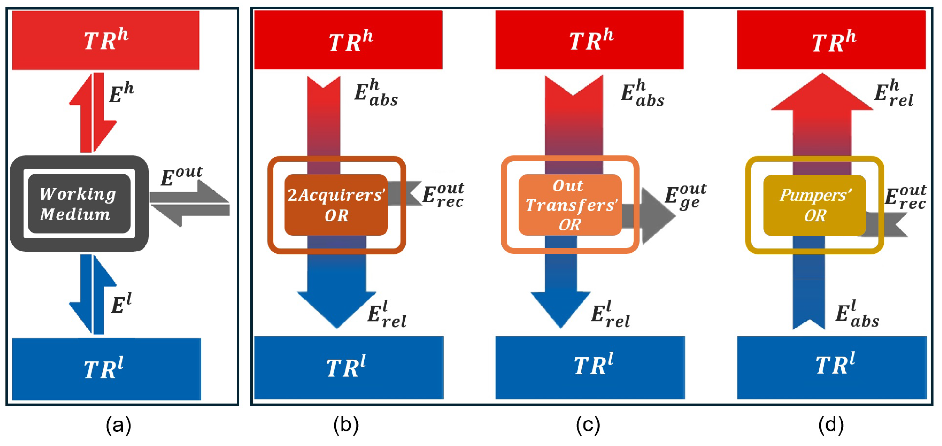
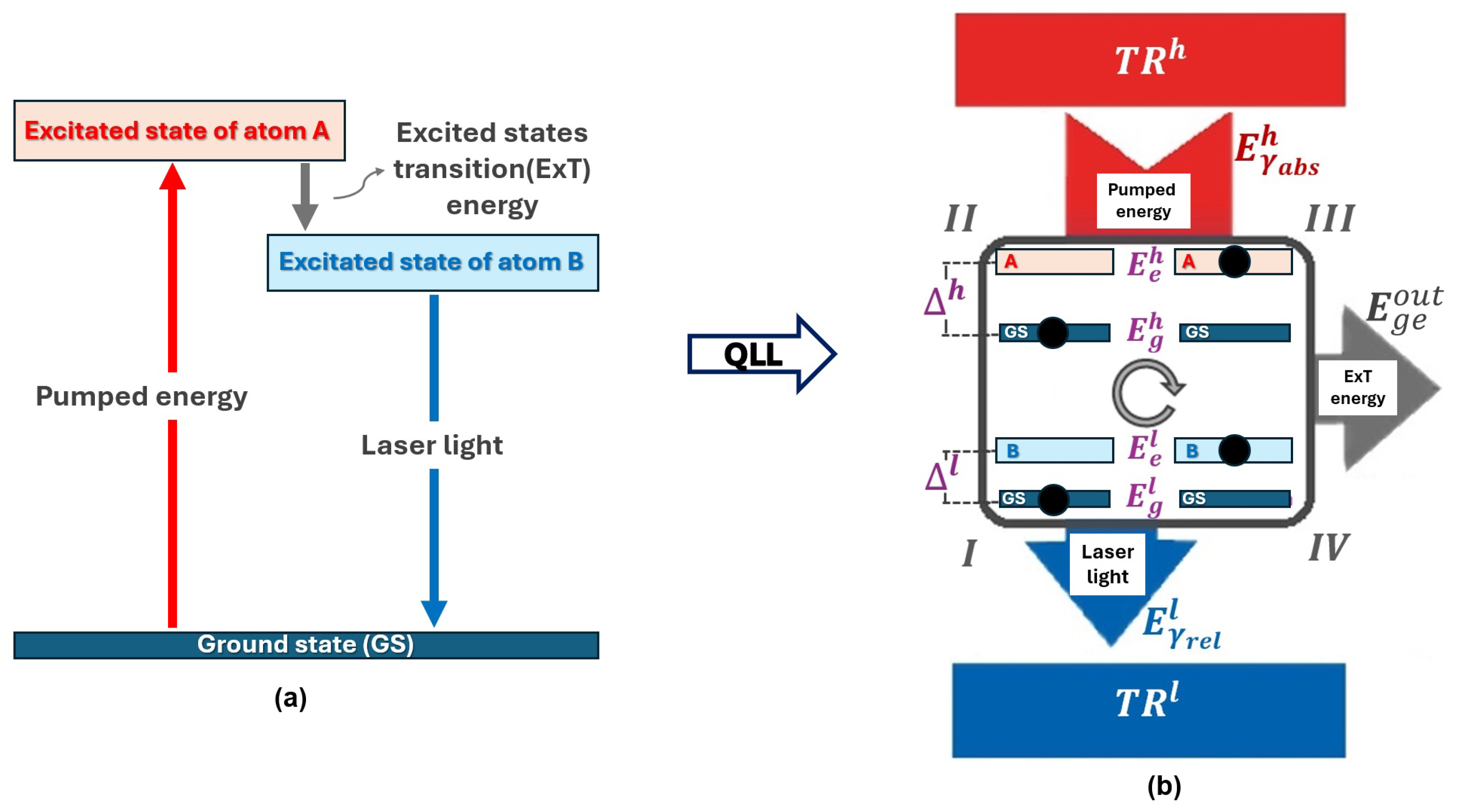
2.1. General Definition of QTMs: Functions and Energy Exchanges

A QTM is fundamentally a device that operates in cycles with a quatum system as its working medium connected to two TRs—one at a higher temperature T h (denoted as T R h ) and the other at a lower temperature T l ( T R l ), that is T h > T l . The working medium mediates energy exchanges between T R h , T R l and the environment external to the QTM. The main purpose of QTMs is to promote a specific type of energy transfer while simultaneously acquiring energy from at least one source.
The schematic of a generic QTM is shown in Figure 1a. E h and E l represent the total energy exchanged with T R h and T R l , respectively. We introduce the concept of a QTM’s outside exchange energy (denoted as E o u t ), which represents all energy exchanges by the QTM that are not directly absorbed from or released to T R h or T R l , i.e., energy exchanged with the environment external to the QTM. Specifically, from energy conservation law, we have
E o u t = E h + E l .
Since our calculations are based on the most widely accepted standard in the literature for studying QEN, we define
E a b s T R > 0 and E r e l T R < 0 ,
where E a b s T R refers to the energy absorbed from T R h or T R l , and E r e l T R refers to the energy released to these TRs.
In the same way, we define
E g e o u t > 0 and E r e c o u t < 0 ,
where E g e o u t corresponds to the net generation of energy transferred to the QTM’s outside, while E r e c o u t signifies the net reception of energy from the QTM’s outside. In other words, E o u t may originate from or be sent to outside the T R h –working medium– T R l axis, which is essentially the QTM.
To distinguish the different types of energy exchanges occurring in a QTM cycle, we have standardized the use of specific verbs for each exchange process. Energy acquired from TRs is described as “absorbed”, while energy drawn from the QTM’s outside is referred to as “received”. Conversely, energy directed toward the TRs is termed “released”, and energy sent to the QTM’s outside is called “generated”. This standardization not only facilitates the recognition of each energy exchange event but also helps prevent confusion throughout the analysis. As defined above, energy “absorbed” from the TRs or generated to QTM’s outside is treated as positive, whereas energy received from the QTM’s outside or released to TRs is considered negative.

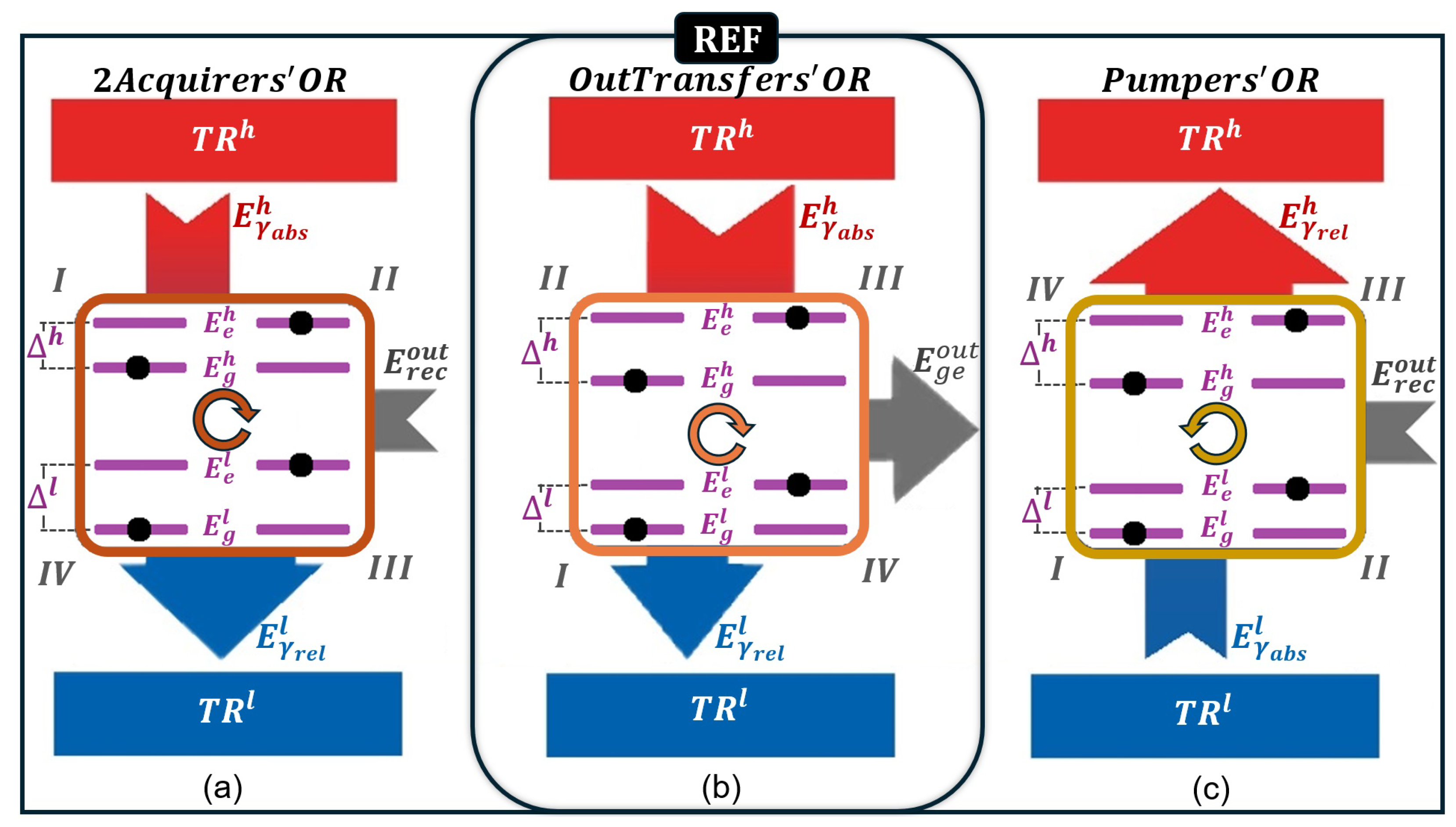
2.2. Defining the Operational Regions of a Working Medium and Their Corresponding QTMs

We define the operational region of a working medium as the set of configurations that enable it to exchange energy with T R h , T R l and the environment external to the QTM in a manner consistent with the fundamental principles of thermodynamics. A QTM operates within a specific operational region when its behavior aligns with the defining characteristics of that operational region. The distinction between QTMs in the same operational region is determined by their prioritization of energy exchanges and their primary energy sources.
The general schematic in Figure 1a illustrates all possible energy exchanges between the working medium, T R h , T R l , and the QTM’s outside.
The schematic reveals that only three distinct operational regions emerge, each satisfying both the law of energy conservation and the second law of thermodynamics, while also allowing for cyclic processes. In Appendix A, we define and analyze the other hypothetical configurations that violate these laws.
The first operational region is referred to as the Bi-Acquirers’ Operational Region (2Acquirers’OR). In this configuration, the QTM receives E r e c o u t from the external environment, absorbs E a b s h from T R h , and releases E r e l l to T R l . A key feature of this regime is that the magnitude of absorbed energy from the hot reservoir is smaller than the energy released to the cold one, i.e., E a b s h < E r e l l .
This operational region is unique in that it allows for two possible energy sources, leading to two subregions: 2Acqout and 2Acqh. In 2Acqout, QTMs use E r e c o u t as their primary energy source. Two configurations are identified here: the quantum cooler (QCO), which emphasizes the absorption of E a b s h , and the quantum heater (QHT), which emphasizes the release of E r e l l .
QTMs in the 2Acqh subregion instead use E a b s h as their main energy source. Two machines fall into this category: the quantum thermal damper (QDP), which prioritizes the reception of E r e c o u t , and the quantum heating optimizer (QHO), which prioritizes the release of E r e l l .
Figure 1c illustrates the Outside Transfers’ Operational Region (OutTransfers’OR). QTMs operating within the OutTransfers’OR absorb E a b s h from T R h and release E r e l l to T R l , where E a b s h > E r e l l . In this process, E g e o u t is generated. The well-studied QEN, which prioritizes the generation of E g e o u t , and the newly designed quantum thermal laser- like (QLL), which prioritizes the release of E r e l l , are QTMs operating within this region. As its name suggests, we believe that the QLL provides a more accurate representation of the laser functionality as a QTM (see Section 3.8).
Finally, Figure 1d illustrates the Thermal Pumpers’ Operational Region (Pumpers’OR). QTMs in this operational region operate in a cycle opposite to that of the QTMs in the OutTransfers’OR. Here, E r e l h is released from T R h , and E a b s l is absorbed from T R l , where E r e l h > E a b s l . This process does not occur naturally between the TRs and requires the input of E r e c o u t from the QTM’s outside to enable the exchange. It is important to emphasize that E a b s l cannot be considered an energy source, as doing so would contradict the second law of thermodynamics. Two QTMs operate within the Pumpers’OR: the well-known QRE, which is essentially a cold pumper and prioritizes the absorption of E a b s l from T R l , and the quantum heat pumper (QHP), which prioritizes the release of E r e l h to T R h .
Although terms such as “cold”, “heat”, or “refrigerator” may appear inconsistent with quantum-level processes, we choose to retain this classical nomenclature due to its widespread use in QTM studies.
We are dealing with a working medium coupled to two TRs. Consequently, if the working medium receives energy from one TR, it must release energy to the other for the cycle to occur, that is,
E a b s l E r e l h , E a b s h E r e l l .
Moreover, since the aim is to present the results for all operational regions of a working medium in a single graph, and given the definition in Equation (2) and the implications summarized in Equation (4), we can express a common equation between E h and E l for all operational regions as follows
E h E l = α 2 .
where we named α 2 as the thermal high–low energy ratio.
Therefore, considering the previously defined energy conventions for all operational regions, we conclude that 0 < α 2 < 1 corresponds to the relationship between E h and E l in the 2Acquirers’OR, while α 2 > 1 represents this relationship in the OutTransfers’OR and Pumpers’OR.

2.3. Classical and Quantum Energy Relationships

The first law of thermodynamics, when applied to a classical working medium, is expressed as
d U = δ Q δ W ,
which, in quasi-static processes, becomes
Δ U = Q W ,
where Δ U is the change in internal energy of the classical working medium, Q = Q a b s + Q r e l is the total heat exchanged with the TRs, and W = W g e + W r e c denotes the net work exchanged with the machine’s external environment.
According to Equation (7), both the heat absorbed from the TRs, Q a b s , and the work generated by the classical working medium, W g e , are considered positive. Conversely, the heat released to the TRs, Q r e l , and the work received from the external environment, W r e c , are negative.
Because classical thermal machines operate cyclically, implying Δ U = 0 , Equation (7) simplifies to W = Q . Substituting Q = Q a b s + Q r e l , we obtain
W = Q a b s + Q r e l .
We do not substitute W = W g e + W r e c into Equation (8) because for most classical thermal machines, distinguishing between W g e and W r e c is unnecessary. In typical analyses, W = W g e is used when the net work is positive, and W = W r e c is used when it is negative.
For instance, when evaluating the efficiency of a thermal engine, the critical question is: How much useful work can it perform? In such cases, in Equation (8), W represents the net or useful work produced by the classical working medium in each engine cycle, specifically W = W g e .
By comparing Equation (1) with Equation (8), and considering Equation (4), we can conclude that
E o u t QTM W CTM , E h + E l QTM Q CTM , and E a b s T R + E r e l T R QTM Q CTM ,
where CTM is an acronym for the classical thermal machine.
The last equivalence above can also be expressed as
E a b s T R + E r e l T R QTM Q a b s + Q r e l CTM , or even E a b s T R QTM Q a b s CTM , and E r e l T R QTM Q r e l CTM .
It is important to note that in operational regions such as the Pumpers’OR and 2Acquirers’OR, the QTM operates under a negative work condition. In these scenarios, as seen in the previous section, the machine requires a net energy input from the outside-QTM environment ( E r e c o u t < 0 ), which is directly analogous to the classical concept of negative work ( W r e c < 0 ) associated with refrigeration and pumping processes. This stands in contrast to QTMs operating within the OutTransfers’OR where the machine delivers energy to the outside environment ( E g e o u t > 0 ), corresponding to a positive work condition ( W g e > 0 ). This distinction between positive and negative work modes is essential for understanding the role and operational purpose of each QTM design proposed in this framework.
Despite the formal equivalence between work and heat in terms of energy exchanges described in this paper, maintaining our generalized definitions and nomenclature for these quantities is essential to ensure a comprehensive analysis of QTMs.

3. Efficiency Calculation and Carnot Efficiency
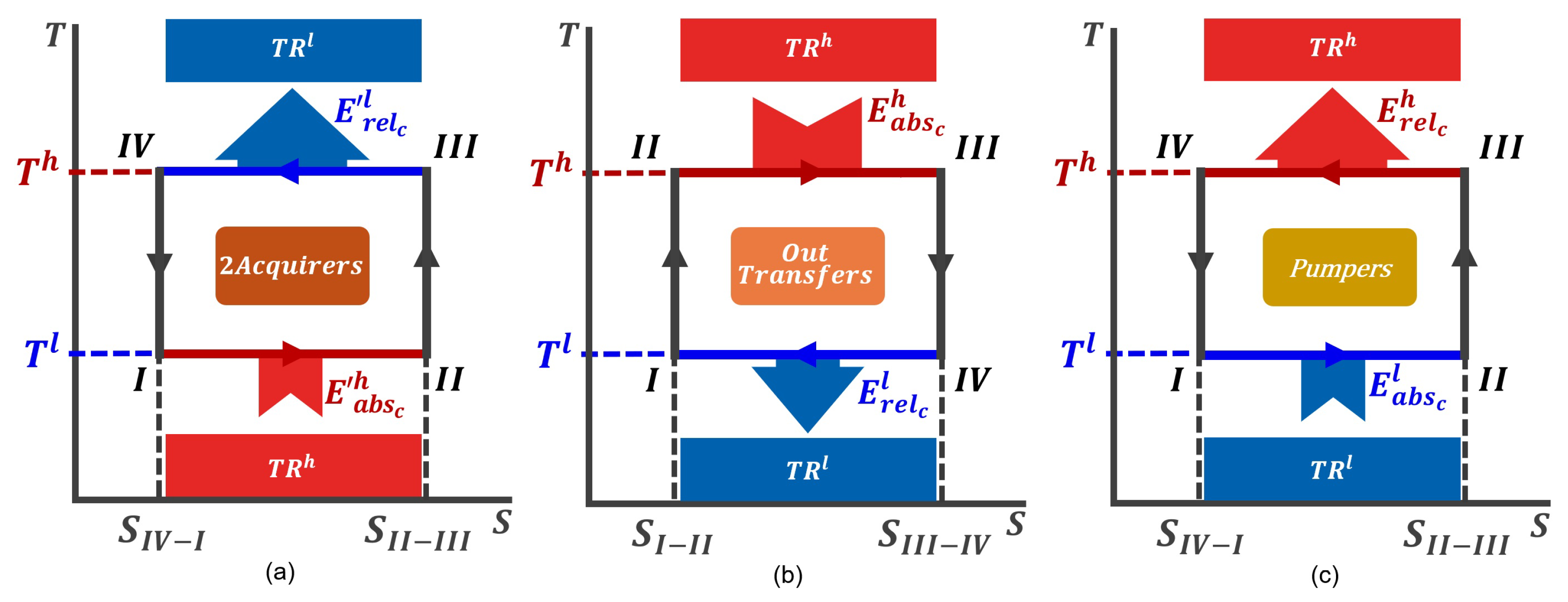
Typically, efficiency is denoted by the symbol η or ε , and the coefficient of performance by the symbol COP, depending on how the QTM operates. For convenience, we adopt the term “efficiency” and use the symbol ε to represent both concepts, as their distinction will remain clear from context throughout the manuscript.
In general, the QTM efficiency, ε QTM , is defined as
ε QTM = E target E available ,
where E target is the energy that the QTM prioritizes, and E available is the main energy source required for the QTM to operate.
Likewise, the QTM Carnot efficiency, ε QTM c , is expressed as
ε QTM c = E target c E available c ,
where E target c and E available c refer to the energy exchange and source under Carnot-cycle operation.
The efficiency expressions in Equations (11) and (12) are well established. However, the proposed classification of operational regions and the introduction of new QTM types call for a broader understanding of the role and behavior of the Carnot efficiency function ε QTM c .
The design of any QTM, which necessarily involves interaction between the working medium and both T R h and T R l , imposes constraints on the magnitude of exchanged energy. As illustrated in Figure 1, the values of E l and E h are bounded by the finite temperatures of the reservoirs. These bounds are theoretically set by the Carnot-cycle operation, which represents the QTM’s optimal efficiency configuration.
Therefore, we define ε QTM c as the limiting efficiency for a QTM in any cycle. It is important to highlight that this definition is comprehensive: the Carnot efficiency may represent either a maximum or a minimum value of ε QTM , depending on the QTM configuration. The implications of this will become clear in subsequent analyses.

3.1. Carnot Cycle

Figure 2 illustrates the three operational regions in temperature–entropy (T-S) diagrams, representing all potential configurations for a QTM operating in the Carnot cycle. The notation I–II-III–IV designates the thermodynamic states and the direction of the cycle for each operational region, establishing a standard framework for analysis across the diagrams in this work. T h and T l correspond to the maximum and minimum temperatures reached by the QTMs during the cycle, which align with the temperatures of the thermal reservoirs T R h and T R l , respectively.
For simplifying several aspects of our analysis, we define the high–low temperature ratio, θ 2 , as
θ 2 = T h T l ,
where θ 2 > 1 for any QTM configuration.
In the previous section, we concluded that comparing Equation (1) with Equation (8) reveals that the energy exchanges between the working medium and the thermal reservoirs, T R h and T R l , are analogous to classical heat exchanges. This analogy is well supported in the literature (see [18,21]), forming a basis for applying the following classical relationship between entropy (S), temperature (T), and heat (Q), in the study of quantum systems:
δ Q = T d S .
Equation (14) enables the calculation of entropy variation for the working medium in any operational region, assuming Q given by Equation (10).
The QTMs operating within the 2Acquirers’OR follow a counterclockwise Carnot cycle, as shown in Figure 2a. During this process, E r e l c l is released to T R l in an isothermal stroke at T h , which exceeds the E a b s c h absorbed from T R h during an isothermal stroke at T l . Essentially, the reception of E r e c o u t from the machine’s outside positions the QTM such that the working medium reaches its maximum temperature ( T h ) just before releasing energy to T R l .
In the Carnot cycle, the entropy variation of the working medium for QTMs in the 2Acquirers’OR is expressed as
Δ S 2 Acq Carnot = I I I d E a b s c h T l + I I I I V d E r e l c l T h .
In the strokes II–III and IV–I, there is no entropy change, as these are adiabatic processes, and there is no entropy change in a closed cycle. Thus, considering that the strokes I–II and III–IV are quasi-static isothermal processes, from Equations (13) and (15), we have
T h T l = E r e l c l E a b s c h = θ 2 .
The QTMs in the OutTransfers’OR work in a clockwise cycle (Figure 2b), absorbing the energy E a b s c h during an isothermic stroke at T h and releasing the energy E r e l c l during an isothermic stroke at T l .
Building on the same analysis that led to Equation (15), we obtain the following result for the entropy variation of the QTMs’ working medium in the OutTransfers’OR
Δ S OutT Carnot = I I I I I d E a b s c h T h + I V I d E r e l c l T l ,
and, from Equations (13) and (17), we have
T h T l = E a b s c h E r e l c l = θ 2 .
Figure 2c shows the counterclockwise cycle for the QTMs in the Pumpers’OR, where E a b s c l is absorved during an isothermic stroke at T l and E r e l c h is released during an isothermic stroke at T h . The Carnot cycle that follows by these QTMs is the exact opposite to the Carnot cycle followed by the QTMs in the OutTransfers’OR, and the working medium’s entropy variation is given by
Δ S Pump Carnot = I I I d E a b s c l T l + I I I I V d E r e l c h T h ,
and
T h T l = E r e l c h E a b s c l = θ 2 .
Next, we apply these results to calculate the efficiency ε QTM and the Carnot efficiency ε QTM c for each type of QTM operating within its respective operational region. These calculations provide insight into how different configurations and energy exchanges impact the overall performance of QTMs.

3.2. Bi-Acquirers’ Operational Region

In the 2Acquirers’OR, QTMs can use two distinct acquired energies as their primary source: E r e c o u t or E a b s h . This results in two subregions: 2Acqout and 2Acqh. QTMs operating within the 2Acqout subregion, such as the QCO and the QHT, use E r e c o u t as the main energy source. Conversely, QTMs in the 2Acqh subregion, like the QDP and QHO, use E a b s h .
Both QCO and QHT have already been covered in existing publications. However, their characterizations and nomenclatures remain inconsistently defined, and they are often used arbitrarily, which obstructs a broader understanding of their actual potential and limitations.
The specific characteristics and operational principles of these machines will be analyzed in detail below with the aim of clarifying their classifications and highlighting their distinct thermodynamic roles within the 2Acquirers’OR.

3.2.1. Quantum Cooler

  • QCO Operational Mode
    Energy priority: E target = E a b s h .
    Energy source: E available = E r e c o u t .
  • QCO Efficiency
    From Equation (11), we can write
    ε QCO = E a b s h E r e c o u t = E a b s h E a b s h + E r e l l = 1 E r e l l E a b s h 1
    whose substitutions were based on Equations (1) and (2).
    Using Equation (5), in Equation (21), we have
    ε QCO = 1 1 α 2 1 .
  • QCO Carnot Efficiency
    From Equations (1), (2) and (12), we can write
    ε QCO c = E a b s c h E r e c c E = 1 E r e l c l E a b s c h 1 .
    Using Equation (16) in Equation (23), we have
    ε QCO c = 1 T h T l 1 = 1 θ 2 1 .
    It is very important to emphasize that θ depends exclusively on the ratio between T h and T l , as given by Equation (13).
  • Analysis of Limits for ε QCO and α QCO 2 Values
    Equation (5) is defined such that 0 < α 2 < 1 represents the relationship between E h and E l for any QTM within the 2Acquirers’OR. The implication of this restriction in Equation (22) is as follows:
    When α 2 0 , ε QCO 0 .
    When α 2 1 , ε QCO .
    There is no impediment to ε QCO 0 . Therefore, there are also no restrictions on the minimum value of α , allowing for
    α QCO m i n 2 = 0 .
    However, when any ε QTM , it is necessary to impose a limit, which is associated to the ideal capacity of the TRs to supply and absorb energy from the working medium, i.e.,
    ε QCO m a x = ε QCO c | α 2 1 ,
    where α 2 has a maximum value for the QCO, obtained by substituting Equations (22) and (24) into the above equation, such that
    1 1 α QCO m a x 2 1 = 1 θ 2 1 , α QCO m a x 2 = 1 θ 2 .
For all subsequent calculations of ε QTM and ε QTM c , the substitutions from Equations (1), (2) and (5) through (13) will be applied implicitly. In the specific case of calculating ε QTM c within the 2Acquirers’OR, the substitution based on Equation (16) will also be considered implicit.

3.2.2. Quantum Heater

  • QHT Operational Mode
    Energy priority: E target = E r e l l .
    Energy source: E available = E r e c o u t .
  • QHT Efficiency
    ε QHT = E r e l l E r e c o u t = 1 1 + E a b s h E r e l l = 1 1 α 2 .
  • QHT Carnot Efficiency
    ε QHT c = 1 1 + E a b s c h E r e l c l = 1 1 T l T h = 1 1 1 θ 2 .
  • Analysis of Limits for ε QHT and α QHT 2 Values
    For QHT, 0 < α 2 < 1 . In Equation (28), the following apply:
    When α 2 0 , ε QHT 1 .
    When α 2 1 , ε QHT .
    Since it is allowed for ε QHT 1 , we have
    α QHT m i n 2 = 0 .
    On the other hand,
    ε QHT m a x = ε QHT c | α 2 1 .
    As derived for the QCO, the value of α 2 reaches a maximum for the QHT, determined by inserting Equations (28) and (29) into the Equation (31), resulting in
    α QHT m a x 2 = 1 θ 2 .

3.2.3. Quantum Thermal Damper

Currently, no mention in the literature addresses a QTM with the specific configuration proposed for the QDP. The main priority of this QTM is to receive E r e c o u t from outside. As we will demonstrate, ε QDP is inversely related to that of the QEN ( ε QEN ). While a QEN generates useful E g e o u t to the outside, the QDP prioritizes extracting E r e c o u t from the outside, functioning as a quantum damper.
  • QDP Operational Mode
    Energy priority: E target = E r e c o u t .
    Energy source: E available = E a b s h .
  • QDP Efficiency
    ε QDP = E r e c o u t E a b s h = E r e l l E a b s h 1 = 1 α 2 1 .
  • QDP Carnot Efficiency
    ε QDP c = E r e l l E a b s h 1 = T h T l 1 = θ 2 1 .
  • Analysis of Limits for ε QDP and α QDP 2 Values
    For QDP, 0 < α 2 < 1 . In Equation (33), the following apply:
    When α 2 0 , ε QDP .
    When α 2 1 , ε QDP 0 .
    In this case, we observe that ε QDP 0 is also allowed, and it is also allowed for α 2 to reach its maximum value, i.e.,
    α QDP m a x 2 = 1 .
    At the opposite limit,
    ε QDP m a x = ε QDP c | α 2 0 .
    From the above analyses, it is concluded that ε QDP reaches its maximum at a minimum value of α 2 , which is determined by substituting Equations (33) and (34) into Equation (36), such that
    α QDP m i n 2 = 1 θ 2 .

3.2.4. Quantum Heating Optimizer

The transfer of energy from T R h to T R l is a natural process consistent with the second law of thermodynamics and occurs even without the intervention of a QTM. A QHO facilitates this process by prioritizing the release of E r e l l to T R l , while absorbing E a b s h from T R h . Although E r e c o u t from the outside is not the QTM’s primary energy source, its presence enhances the energy released to T R l without affecting the energy absorbed from T R h , thus improving the QTM’s overall efficiency.
As with the QDP, this QTM is not mentioned in the existing literature. Despite its simpler configuration, understanding all potential QTM designs remains crucial for a comprehensive theoretical investigation.
  • QHO Operational Mode
    Energy priority: E target = E r e l l .
    Energy source: E available = E a b s h .
  • QHO Efficiency
    ε QHO = E r e l l E a b s h = E r e l l E a b s h = 1 α 2 .
  • QHO Carnot Efficiency
    ε QHO c = E r e l l E a b s h = T h T l = θ 2 .
  • Analysis of Limits for ε QHO and α QHO 2 Values
    For the QHO, 0 < α 2 < 1 . In Equation (38), the following apply:
    When α 2 0 , ε QHO .
    When α 2 1 , ε QHO 1 .
    Therefore,
    α QHO m a x 2 = 1 ,
    and
    ε QHO m a x = ε QHO c | α 2 0 ,
    which, from the substitution of Equations (33) and (34) into Equation (41), gives the following:
    α QHO m i n 2 = 1 θ 2 .

3.3. Outside Transfers’ Operational Region

This is the most extensively studied and cited operational region in the literature, as it includes the quantum engine (QEN). However, we propose that an alternative QTM design, the quantum laser-like machine (QLL), can also be constructed within this region. As discussed in Section 3.8, we argue that the QLL provides a more accurate description of how the laser operates.

3.3.1. Quantum Thermal Engine

  • QEN Operational Mode
    Energy priority: E target = E g e o u t .
    Energy source: E available = E a b s h .
  • QEN Efficiency
    ε QEN = E g e o u t E a b s h = 1 + E r e l l E a b s h = 1 1 α 2 .
    The efficiency of a monatomic ideal gas acting as the working medium in a classical thermal engine, ε C T E , operating under the Otto cycle, is given by
    ε CTE = 1 1 ρ 2 3 ,
    where ρ is the compression ratio, which is defined as
    ρ = volume before compression volume after compression .
    By comparing Equations (43) and (44), we observe that α plays a role analogous to the compression ratio in the QEN operating under the Otto cycle. As demonstrated in Section 4, this correspondence holds for all QTMs using two-level systems as their working medium.
  • QEN Carnot Efficiency
    ε QEN c = 1 + E r e l c l E a b s c h = 1 T l T h = 1 1 θ 2 .
  • Analysis of Limits for ε QEN and α QEN 2 Values
    As defined in Equation (5), α 2 > 1 expresses the relationship between E h and E l for any QTM in the OutTransfers’OR. From Equation (43), we observe the following limiting behaviors:
    When α 2 1 , ε QEN 0 .
    When α 2 , ε QEN 1 .
    Therefore, the minimum efficiency corresponds to
    α QEN m i n 2 = 1 ,
    However, it is well known that ε QEN 1 implies E r e l l 0 , which would violate the second law of thermodynamics for a thermal engine. The efficiency limit is ultimately determined by the ideal capacity of the thermal reservoirs to supply and absorb energy from the working medium. Accordingly,
    ε QEN m a x = ε QEN c | α 2 ,
    and
    α QEN m a x 2 = θ 2 .

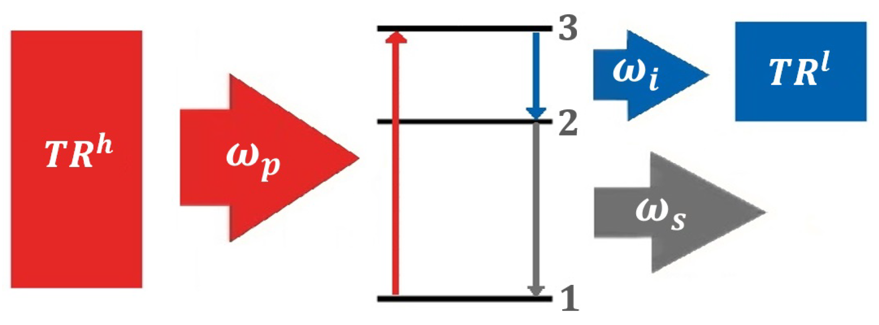
3.3.2. Quantum Thermal Laser-like

  • QLL Operational Mode
    Energy priority: E target = E r e l l .
    Energy source: E available = E a b s h .
  • QLL Efficiency
    ε QLL = E r e l l E a b s h = E r e l l E a b s h = 1 α 2 .
  • QLL Carnot Efficiency
    ε QLL c = E r e l c l E a b s c h = T l T h = 1 θ 2 .
  • Analysis of Limits for ε QLL and α QLL 2 Values
    For QLL, α 2 > 1 . In Equation (50), the following apply:
    When α 2 1 , ε QLL 1 .
    When α 2 , ε QLL 0 .
    QLL is the only QTM for which ε QLL c must bound the minimum value of ε QLL , as E r e l l 0 , when ε QLL 0 .
    Therefore,
    ε QLL m i n = ε QLL c | α 2 .
    The data above indicate that ε QLL reaches its minimum at the maximum value of α 2 . This value can be determined by substituting Equations (50) and (51) into Equation (52), as follows
    α QLL m a x 2 = θ 2 .
    Conversely, there are no constraints on ε QLL 1 , and thus,
    α QLL m i n 2 = 1 .

3.4. Thermal Pumpers’ Operational Region

As previously mentioned, in the Pumpers’OR, energy transfer between the thermal reservoirs (TRs) does not follow the thermodynamically natural direction. The presence of E r e c o u t is crucial, as it enables the QTM to extract energy from T R l and release it into T R h . The quantum refrigerator (QRE) and the quantum heat pumper (QHP) are the QTMs operating within this region. While the QRE is well established in the current literature—similarly to QCO and QHT—a proper definition of the QHP’s characteristics and the adoption of standardized nomenclature are still required.

3.4.1. Quantum Refrigerator

  • QRE Operational Mode
    Energy priority: E target = E a b s l .
    Energy source: E available = E r e c o u t .
  • QRE Efficiency
    ε QRE = E a b s l E r e c o u t = 1 1 + E r e l h E a b s l = 1 α 2 1 .
  • QRE Carnot Efficiency
    ε QRE c = 1 1 + E r e l c h E a b s c l = 1 T h T l 1 = 1 θ 2 1 .
  • Analysis of Limits for ε QRE and α QRE 2 Values
    For the QRE, α 2 > 1 . From Equation (55), the following apply:
    When α 2 1 , ε QRE .
    When α 2 , ε QRE 0 .
    In this case, we have
    α QRE m a x 2 ,
    since no physical constraint prevents ε QRE 0 .
    At the opposite limit, we obtain
    ε QRE m a x = ε QRE c | α 2 1 .
    As also found for QTMs in the 2Acqh subregion, ε QRE reaches its maximum at the minimum value of α 2 . Substituting Equations (55) and (56) into Equation (58), we find
    α QRE m i n 2 = θ 2 .

3.4.2. Quantum Heat Pumper

  • QHP Operational Mode
    Energy priority: E target = E r e l h .
    Energy source: E available = E r e c o u t .
  • QHP Efficiency
    ε QHP = E r e l h E r e c o u t = 1 1 + E a b s l E r e l h = 1 1 1 α 2 .
  • QHP Carnot Efficiency
    ε QHP c = 1 1 + E a b s c l E r e l c h = 1 1 T l T h = 1 1 1 θ 2 .
  • Analysis of Limits for ε QHP and α QHP 2 Values
    For the QHP, α 2 > 1 . From Equation (60), the following apply:
    When α 2 1 , ε QHP .
    When α 2 , ε QHP 1 .
    Therefore, as in previous analyses, we have
    α QHP m a x 2 ,
    ε QHP m a x = ε QHP c | α 2 1 ,
    and
    α QHP m i n 2 = θ 2 .

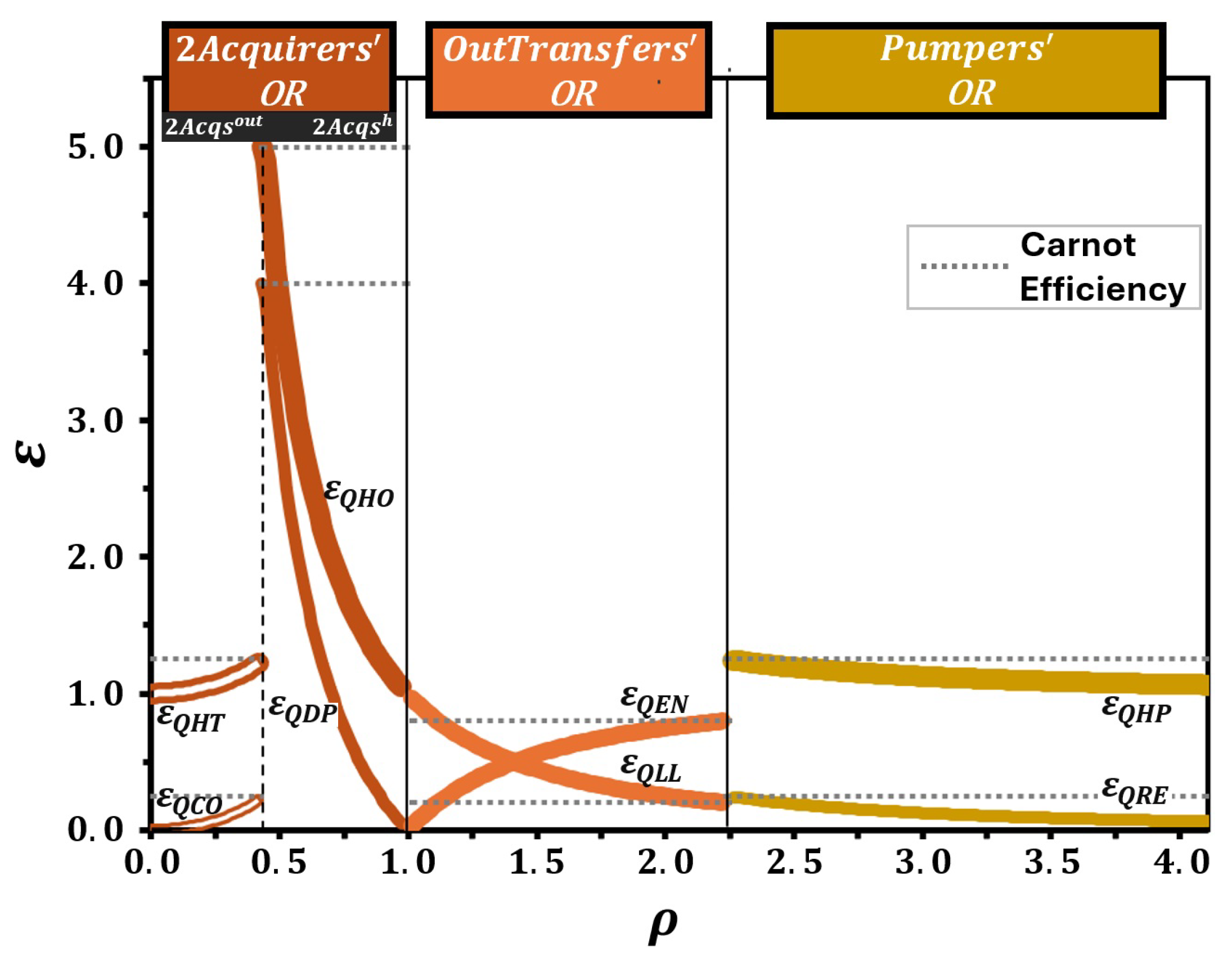
3.5. Efficiency Relationships Within the Same Operational Region

The relationships between the efficiencies of QTMs within each operational region can be inferred directly from the schematic representations in Figure 1b–d. Moreover, the analytical expressions derived for the efficiencies of all QTMs allow for precise deductions of these relationships, as described below.
  • Bi-Acquirers’ Operational Region
    From Equations (22) and (28), and from Equations (33) and (38), we obtain
    ε QHT ε QCO = 1 1 α 2 1 1 α 2 1 = 1 ,
    and
    ε QHO ε QDP = 1 α 2 1 α 2 1 = 1 ,
    which leads to
    ε QHT > ε QCO ,
    and
    ε QHO > ε QDP .
  • Outside Transfers’ Operational Region
    The relationship among efficiencies in the OutTransfers’OR is different. From Equations (43) and (50), we have
    ε QEN + ε QLL = 1 1 α 2 + 1 α 2 = 1 .
    In this case, neither QEN nor QLL dominates in efficiency. Equation (69) also implies that neither can exceed unity in efficiency.
  • Thermal Pumpers’ Operational Region
    From Equations (55) and (60), we obtain
    ε QHP ε QRE = 1 1 1 α 2 1 α 2 1 = 1 ,
    leading to
    ε QHP > ε QRE .

3.6. Thermal High–Low Energy Ratio Values at Operational Region Intersections

Based on the results obtained in the previous subsections regarding the limiting values of α 2 for each QTM, we can define the values that characterize the intersections between operational regions, including the boundary between the two subregions in the 2Acquirers’OR.
  • 2 A c q o u t - 2 A c q h Intersection
    Comparing Equations (27), (32), (37) and (42), we conclude that the value of α 2 at the intersection between the 2 Acq o u t and 2 Acq h subregions is
    α 2 Acq o u t 2 Acq h 2 = 1 θ 2 .
  • 2 A c q u i r e r s - O u t T r a n s f e r s Intersection
    The value of α 2 at the intersection between the 2 A c q u i r e r s and O u t T r a n s f e r s operational regions is
    α 2 Acq OutT 2 = 1 ,
    since α 2 Acq m a x 2 = α OutT m i n 2 = 1 (see Equations (35), (40), (47) and (54)).
  • O u t T r a n s f e r s - P u m p e r s Intersection
    From Equations (49), (53), (59) and (64), we obtain
    α OutT Pump 2 = θ 2 .
Table 1 summarizes the findings from this study, providing a comprehensive reference for any QTM whose working medium operates between T R h and T R l , and it is governed by principles similar to those outlined in this work.
In the next section, we apply these results to analyze two-level quantum systems as the working medium of QTMs operating under the Otto cycle.
Based on the proposed operational regions and subregions, Figure 3 illustrates the possible configurations of a two-level quantum system as the working medium of a QT. Figure 3a–c represent the 2Acquirers’OR, OutTransfers’OR, and Pumpers’OR configurations of the two-level quantum system, respectively.
We treat the OutTransfers’OR configuration as the reference (Figure 3b), from which the subsequent calculations naturally evolve.
As shown in Figure 3b, the two-level quantum system has four possible states. In state I, the particle is in the ground state with energy E g l , and the energy gap between the levels, Δ l , is given by
Δ l = E e l E g l ,
where E e l is the excited energy level in state I. In state II, the particle occupies the ground level of a different dimensional configuration with levels E g h and E e h separated by the gap
Δ h = E e h E g h .
In state III, the system retains the dimensional configuration of state II, but the particle is now in the excited state, E e h . In state IV, the system returns to the dimensional configuration of state I with the particle occupying the excited state E e l .
As detailed in Section 3.7, changes in the dimensional configuration of the two-level system are driven by energy exchanges with the QTM’s external environment ( E o u t ), while transitions between energy levels are mediated by the absorption or emission of photons. These transitions correspond to exchanges with T R h , denoted as E γ h , and with T R l , which is denoted as E γ l .
In the OutTransfers’OR configuration, the system reaches its maximum temperature, T max = T h , after absorbing energy E γ h from T R h , i.e., when in state III. Conversely, it reaches its minimum temperature, T min = T l , after releasing energy E γ l to T R l , in state I.
The state labels across the three operational regions were defined such that state III (I) corresponds to the configuration with the largest (smallest) energy level separation with the particle in the excited (ground) state at temperature T h ( T l ). Note that, as analyzed in Section 3.1, in the 2Acquirers’OR configuration, the system reaches its maximum ( T h ) or minimum ( T l ) temperature immediately before releasing energy to T R l or absorbing energy from T R h , respectively—corresponding to state III ( T h ) or state I ( T l ) in Figure 3a.

3.7. Otto Cycle

A classical thermal machine operating under the Otto cycle consists of two adiabatic and two isochoric strokes. During the adiabatic strokes, no heat is exchanged with the surroundings, and energy variations arise solely from volume changes. In contrast, during the isochoric strokes, the working medium exchanges heat with T R h and T R l , while its volume remains constant.
One of the distinctive features of the Otto cycle is that each stroke involves either work or heat exchange but never both simultaneously. This is particularly valuable for the theoretical study of QTMs, as each stroke corresponds to either an E T R or an E o u t exchange, thus simplifying the analysis.
In any QTM thermodynamic cycle, a wide range of outcomes is possible, largely depending on the nature of the working medium. In our case, the working medium is a two-level quantum system whose thermodynamic behavior is determined by solving the Schrödinger equation to obtain the energy levels associated with quantum transitions during the cycle.
Multilevel quantum systems as the working medium of a QEN operating in the Otto cycle were thoroughly analyzed by Quan et al. [21]. They introduced quantum analogs of heat, δ Q , and work, δ W , for systems with energy eigenvalues E n , where n = 1 , 2 , 3 , . We apply their formalism to our QTMs using the implications of Equations (9) and (10), and the state labels from Figure 3b, as follows:
δ Q abs = δ E γ abs T R = n E n d P n γ abs T R ,
δ Q rel = δ E γ rel T R = n E n d P n γ rel T R ,
δ W = δ E o u t = n P n d E n ,
where in our case, n = g and n = e denote the ground and excited states, respectively.
The occupation probability P n of the n-th energy eigenstate is given by
P n = e E n / ( k B T ) Z ,
with the partition function
Z = n e E n / ( k B T ) .
Assuming quasi-static strokes, Equation (77) gives the absorbed energy E γ abs h in the OutTransfers’OR (Figure 3b) as
E γ abs h = n I I I I I E n d P n = n = g , e E n h P n ( I I I ) P n ( I I ) = E e h P e ( I I I ) P e ( I I ) + E g h P g ( I I I ) P g ( I I ) .
Similarly, from Equation (77), we obtain the released energy:
E γ rel l = n I V I E n d P n = n = g , e E n l P n ( I ) P n ( I V ) = E e l P e ( I ) P e ( I V ) + E g l P g ( I ) P g ( I V ) .
In the Otto cycle, strokes I–II and III–IV are adiabatic, so the occupation probabilities remain unchanged during these transitions:
P n ( I I ) = P n ( I ) = P n l ,
P n ( I V ) = P n ( I I I ) = P n h .
Thus, the calculations use P n l and P n h obtained from states I and III, where the temperatures are known: T ( I ) = T l and T ( I I I ) = T h .
This gives
E γ abs h = E e h ( P e h P e l ) + E g h ( P g h P g l ) = Δ h e E g l / k B T l e E e h / k B T h e E g h / k B T h e E e l / k B T l ( e E g h / k B T h + e E e h / k B T h ) ( e E g l / k B T l + e E e l / k B T l ) ,
E γ rel l = E e l ( P e l P e h ) + E g l ( P g l P g h ) = Δ l e E g l / k B T l e E e h / k B T h e E g h / k B T h e E e l / k B T l ( e E g h / k B T h + e E e h / k B T h ) ( e E g l / k B T l + e E e l / k B T l ) .
Since the released energy is defined as negative, Equation (87) yields a negative result, as expected.
To compute E g e o u t , we use
E g e o u t = E γ abs h + E γ rel l .
Analogous expressions to Equations (86)–(88) can be derived for the 2Acquirers’OR and Pumpers’OR configurations shown in Figure 3a and Figure 3c, respectively.
Thus, we generalize the expressions for any operational region as
E γ h = Δ h e 1 k B T l E g l e 1 k B T l E e h θ 2 e 1 k B T l E g h θ 2 e 1 k B T l E e l e 1 k B T l E g h θ 2 + e 1 k B T l E e h θ 2 e 1 k B T l E g l + e 1 k B T l E e l ,
E γ l = Δ l e 1 k B T l E g l e 1 k B T l E e h θ 2 e 1 k B T l E g h θ 2 e 1 k B T l E e l e 1 k B T l E g h θ 2 + e 1 k B T l E e h θ 2 e 1 k B T l E g l + e 1 k B T l E e l ,
and
E o u t = E h + E l ,
where in Equations (89) and (90), we have used T h = θ 2 T l (from Equation (13)). The results are consistent with the general form of energy balance (Equation (1)) across operational regions.
Finally, the ratio of Equations (89) and (90) gives
E γ h E γ l = Δ h Δ l ,
which, compared to Equation (5), yields
Δ h Δ l = α 2 .
This confirms that α 2 corresponds to the compression ratio ρ (see Equation (45)) for two-level quantum systems operating under the Otto cycle. Therefore, all QTM designs and classifications proposed in this work remain valid provided the energy eigenvalues of the two-level system are known.

3.8. Rethinking the Laser: Beyond the Quantum Engine Classification

More than sixty years ago, Scovil and Schultz-DuBois [19] proposed that the operation of a maser (microwave amplification by stimulated emission of radiation) could be analyzed similarly to a classical thermal engine. The laser (light amplification by stimulated emission of radiation), which directly succeeded the maser, should also operate on the same fundamental principle.
They suggested that a maser could be described as a three-level system that amplifies a signal at frequency ω s , which is driven by a pump at frequency ω p . The surplus energy is released into an idler mode with frequency ω i = ω p ω s . According to Scovil and Schultz-DuBois, the maser functions as a thermal engine if the idler mode is connected to T R l , while the pumping process is supported by T R h , as illustrated in Figure 4. However, their analysis remained preliminary and did not evolve into studies exploring solid-state quantum effects [18].
In this work, we consider the configuration shown in Figure 5a as our model for the laser. Although simplified and non-generic, we argue that the analysis presented here is extensible to other laser configurations as well.
We treat the laser as a QTM composed of two distinct atoms, each contributing two energy levels. The electronic transition between their excited states is interpreted as a change in the dimensional configuration of the system, generating the energy E g e o u t , while the laser light corresponds to the energy E γ l released to T R l . Thus, according to our proposal, the laser operates as a QTM in the OutTransfers’OR, as illustrated in Figure 5b.
Classifying the laser as a QEN raises conceptual inconsistencies. A QEN must prioritize the generation of energy associated with the expansion of the system’s spatial dimensions—which classically corresponds to the performance of mechanical work, W. For multilevel systems, this implies decreasing the energy gap. Hence, if the laser were treated as a QEN, it would have to prioritize the generation of idler-mode energy, which is physically unjustified. Additionally, in solid-state lasers, the energy release can occur via non-radiative relaxation [36], contradicting the notion that such energy is transferred to T R l .
Our proposal is to reclassify the laser as a QLL, a QTM that prioritizes the release of energy E γ l to T R l , which is in accordance with the defining features of this machine type as developed in this paper.
However, the laser does not operate under an Otto cycle, since the occupation probabilities must satisfy Equations (84) and (85)—conditions that are incompatible with the laser’s fundamental requirement: population inversion. This can be achieved, for example, by using two atoms with distinct characteristics. Therefore, it is both expected and desirable that the occupation probabilities in a laser do not satisfy Otto cycle conditions. As a result, the actual thermodynamic cycle of a laser constitutes an interesting direction for future research.

3.9. A Spinless Electron in a One-Dimensional Quantum Ring as the Working Medium of QTMs

Quantum rings are an important example of quantum systems in the physics of low-dimensional materials [34,35]. However, to our knowledge, no studies have been conducted in the context of QTMs for quantum rings. Therefore, in this work, we have chosen the e in a quantum ring as the two-level quantum system working medium. We explore its possible operational regions and the corresponding QTMs operating in the Otto cycle.
According to Viefers et al. [35], the Schrödinger equation for a e in a quantum ring depends solely on the polar angle φ and can be expressed as
2 2 m e r 2 2 φ 2 ψ φ = E ψ φ ,
where r is the quantum ring radius and m e is the effective mass of the electron.
We consider the solutions of Equation (94) in the form ψ ( φ ) = e i m φ , where m is an integer number. The continuity of the wave function ψ ( φ ) at φ = 2 π requires that m be an integer. Using this solution in Equation (94), we can find the energy eigenvalues depending on the quantum number m. These energies are given explicitly by
E m = 2 2 m e r 2 m 2 ,
where m = 1 , 2 , 3 , .
Figure 3 effectively illustrates the three distinct operational regions of a QTM based on an e in a quantum ring with the understanding that the system’s dimensional configuration changes are driven by variations in the radius of the quantum ring.
Since Equation (95) represents the energy eigenvalues of our quantum system, we can express the energy as
E g l = 2 2 m e r l 2 , E e l = 4 2 2 m e r l 2
and
E g h = 2 2 m e r h 2 , E e h = 4 2 2 m e r h 2 ,
where m = 1 corresponds to the ground energy level (Equation (96)), and m = 2 corresponds to the excited energy level (Equation (97)). Here, r l and r h denote the quantum ring radius when the energy gaps are Δ l and Δ h , respectively. The ratio Δ h / Δ l can be derived from Equations (75) and (76), and compared with Equation (93), which yields
Δ h Δ l = r l r h 2 = α 2 .
Since our system is one-dimensional and changes in its dimensional configuration arise from variations in the radius r, the compression ratio is expected to be defined by the relation
ρ = radius before distancing energy levels radius after distancing energy levels .
Therefore, we conclude that for the e in a quantum ring acting as the working medium,
α = ρ = r l r h ,
where in accordance with Equation (93), we can take α = α .
Equation (100) can also be used to rewrite the Equation (97) as
E g h = ρ 2 2 2 m e r l 2 , E e h = 4 ρ 2 2 2 m e r l 2 .
For the calculations and analyses that follow, we use the following experimental parameters: T l = 1 K , θ 2 = 5 , and r l = 100 nm .
Table 2 presents the results derived from the expressions summarized in Table 1, for e in a quantum ring as the working medium, functioning between T R h and T R l in the Otto cycle.
The graph in Figure 6 illustrates the energies as a function of the compression ratio ρ , normalized by the maximum energy value, for the three possible operational regions of the system. The dashed lines represent the energies exchanged with the TRs, where blue circles indicate the energy exchanged with T R l ( E γ l ) and red squares represent the energy exchanged with T R h ( E γ h ). The solid gray line denotes the energy exchanged with the QTM’s outside ( E o u t ). These energy values are calculated using Equations (89)–(91) by substituting the energy levels from Equations (96) and (101). The solid vertical lines divide the graph into three distinct operational regions. The attached table helps identify these regions by analyzing the allowed ρ values as well as whether the energies involved are positive—indicating absorption (for TRs) or generation (for the QTM’s outside)—or negative—indicating release (for TRs) or reception (from the QTM’s outside).
Since α = ρ (Equation (100)), the 2Acquirers’OR exists only for 0 < ρ < 1 . Furthermore, we obtain E γ h > 0 , E γ l < 0 , and E o u t < 0 throughout this operational region, indicating that QTMs based on the e in a quantum ring can be constructed in the 2Acquirers’OR for any ρ between 0 and 1. Although the distinction between the 2Acqout and 2Acqh subregions is not visually apparent, Table 2 indicates their intersection at ρ = 0.45 , which is represented by the dashed vertical line in Figure 6.
In contrast, the OutTransfers’OR and Pumpers’OR exist only for ρ > 1 . As shown in Figure 6, for values of ρ near 1, we have E γ h > 0 , E γ l < 0 , and E o u t > 0 , corresponding to the OutTransfers’OR. Beyond a certain value of ρ , the signs of these quantities invert, i.e., E γ h < 0 , E γ l > 0 , and E o u t < 0 , indicating the Pumpers’OR. The boundary between these two operational regions is visually evident, and Table 2 shows that it occurs at ρ = 2.24 .
The intersections between the 2Acquirers’OR and the OutTransfers’OR, as well as between the OutTransfers’OR and the Pumpers’OR, are indicated by solid vertical lines in Figure 6.
The efficiencies of all QTMs based on the e in a quantum ring operating in the Otto cycle were analyzed as a function of ρ , using the data from Table 2 (Figure 7). As in Figure 6, Figure 7 separates the operational regions with solid vertical lines, while dashed lines indicate subregion divisions. The graph clearly shows the values of ε QTM and ε QTM c for each QTM within its respective operational region.
The minimum efficiency for QLL and the maximum efficiencies for all other QTMs are determined at the points where their efficiency curves intersect the dashed horizontal line representing ε QTM c . It is important to note that curve extensions beyond operational limits are omitted to ensure consistency within the valid range of ρ . While a more detailed analysis of these results would be valuable, we believe it is more appropriate for future investigations involving parameter variation and comparative studies. Nevertheless, we are confident that the consistency and accuracy of the results obtained for this system, as summarized in Table 2 and Figure 6 and Figure 7, validate and support our proposed framework.
A detailed examination of Figure 6 demonstrates that its structure closely aligns with results previously reported in the literature for QTMs operating under the Otto cycle with quantum systems as working media. Several studies present graphical representations equivalent to Figure 6, where the energies are plotted as functions of a parameter equivalent to the compression ratio [25,37,38,39,40]. This agreement not only validates the correctness of our model but also reinforces the robustness of the theoretical framework adopted in this work.
However, it is important to emphasize that Figure 6 alone does not reveal the full set of thermodynamic behaviors that the same quantum working medium can exhibit. Specifically, it does not provide sufficient information about the existence, limits, and characteristics of the other QTMs that can be constructed from the same working medium.
This limitation is overcome by the introduction of Figure 7, which substantially expands the scope of information available. Unlike Figure 6, Figure 7 displays the efficiencies of all QTMs associated with the different operational regions and subregions of the working medium. This graphical representation clearly highlights the variety of possible machine designs, making explicit the transitions between them as the control parameter, ρ , varies.
To the best of our knowledge, there is no equivalent figure in the existing literature that consolidates, in a single plot, both the efficiency curves and the comprehensive classification of QTMs based on the same working medium. Therefore, Figure 7 provides an unprecedented perspective that significantly enhances the understanding of the thermodynamic potential of quantum systems. It allows for the identification of operational boundaries, the recognition of the conditions under which each machine operates optimally, and the exploration of transitions between different operational modes—an analysis that is not accessible through the standard efficiency plots typically found in previous studies.
The theoretical insights presented here gain further relevance when considered alongside experimental advances. A laser-cooled ion, confined within the combined electrostatic harmonic potential of a Paul trap and the sinusoidal potential of an optical lattice, serves as an example of an experimental platform for implementing quantum refrigerators, heaters, and engines [22]. Nuclear magnetic resonance (NMR) has emerged as a reliable experimental platform for the realization and investigation of quantum thermal machines, enabling the implementation of heat engines, refrigerators, and protocols exploring energy fluctuations and quantum thermodynamic relations [41]. Our findings suggest that new directions, still at the classical–quantum interface, may be explored to advance and refine studies in quantum thermodynamics, particularly concerning QTMs. For example, the quantum thermal damper (QDP) and the quantum heating optimizer (QHO) are novel proposed QTM configurations. To the best of our knowledge, no experimental realizations have been reported so far. Nonetheless, both represent physically consistent and thermodynamically sound operational modes, which are potentially implementable in specific quantum platforms.
In this regard, Ref. [42] presents a study of quantum Otto engines with spatial curvature dependence, using a quantum harmonic oscillator on a circle as the working substance. Our work could contribute to this line of research, as the different regimes analyzed here could also be explored within that context. Furthermore, it would be particularly interesting to investigate how these regimes are modified through the manipulation of parameters such as the curvature of the ring and the oscillator frequency, or even through the inclusion of a magnetic flux.
Complementarily, Ref. [43] theoretically examines a quantum heat engine (QHE) based on the quantum Otto cycle (QOC), employing a spin–star–chain system model as the working fluid. This system consists of a central atom interacting with multiple Heisenberg spin chains. The study considers three distinct configurations of the working fluid—X, XX, and XYZ—evaluating the work output and heat exchange in each case. The results indicate that the X configuration exhibits the highest efficiency among the three. Moreover, an increase in the relative frequency of the central atom enhances the efficiency in all configurations, although none reaches the ideal Carnot efficiency. By analyzing the plots of work, absorbed heat, and released heat presented in the study, one can identify all the configurations discussed here. This suggests that a further investigation could not only provide a unified description of these regimes but also propose strategies to tune different thermal machines by manipulating the relevant parameters of the systems under consideration.
In Ref. [39], the performance of quantum heat engines of the Otto and Carnot types is compared using a two-spin Heisenberg system as the working substance. The study analyzes how interactions such as Dzyaloshinsky–Moriya and dipole–dipole, as well as the presence of an external magnetic field, affect work extraction and heat exchange in four-stroke thermodynamic cycles. The results show that the Carnot cycle generally produces more useful work than the Otto cycle and that the laws of thermodynamics are upheld. The study also identifies the operational conditions corresponding to different modes of operation, such as engine, refrigerator, and heater. Moreover, all the regimes discussed here can be explored within the context of this work as well as the transitions between them through the manipulation of the parameters involved in this system.
In Ref. [40], an operational regime characterized by Q in < 0 , Q out < 0 and W < 0 is described. This set of signs indicates a passive device that dissipates energy rather than a traditional heat engine. It can be interpreted as a heat dissipator with externally applied work, or as a system that performs no useful work, does not transfer heat from a cold to a hot reservoir—as in a refrigerator—and does not convert heat into work—as in a heat engine (see Appendix A). In other words, it is a system that consumes work and releases heat to two thermal reservoirs without any apparent benefit. In addition to this case, the operational regimes of engine, heater, and refrigerator are also described. This is also an example in which a more in-depth study can be conducted in light of what we propose here, since the necessary ingredients for such an investigation are present. A similar situation occurs in Refs. [44,45], and this can also be found in several previous studies involving quantum thermal machines, considering only the thermal reservoirs involved.
It is worth highlighting that the framework developed in this study is applicable to a wide range of quantum systems, including those whose dynamics are governed by advanced quantum control protocols. For instance, the quantum system explored in Ref. [46] can be naturally interpreted as the working medium of a QTM, while each of the four distinct nonequilibrium protocols, optimized to enhance performance in quantum thermal tasks, corresponds to a possible thermodynamic cycle. This approach not only determines whether the quantum system can indeed function as a working medium but also enables a rigorous assessment of its performance based on the general efficiency expressions developed here. Such an analysis may offer an alternative perspective on the results reported in Ref. [46], particularly in evaluating whether the protocol identified as the most efficient is consistent with the thermodynamic boundaries and operational limits established in this work.

4. Conclusions

This study introduces an innovative framework for analyzing QTMs by distinguishing the different ways in which a working medium exchanges energy with T R h , T R l , and the external environment. It defines the concept of an operational region and proposes new designs of QTMs, including the QDP, QHO, and QLL, which naturally emerge from a detailed analysis of each region. In addition to expanding theoretical perspectives, this work introduces a standardized classification scheme for QTMs, providing a cohesive nomenclature and operational framework that may serve as a foundation for future research and practical implementations.
Our theoretical analysis of previously known QTMs highlights their strong agreement with established predictions, reinforcing the validity and applicability of our framework.
A particularly significant result is the reclassification of the laser. Rather than being considered a QEN, we propose it as a distinct QTM operating in the OutTransfers’OR. Furthermore, results obtained for two-level quantum systems—especially those involving an electron in a quantum ring operating under an Otto cycle—illustrate the robustness of our approach. We identified a broad spectrum of possible QTMs, each exhibiting unique properties and operational efficiencies.
We believe this work makes important contributions to the field of quantum thermodynamics by expanding theoretical insight and opening new avenues for technological development. The proposed classification scheme also brings clarity and cohesion to an area where previous nomenclatures and operational definitions lacked standardization. The framework developed here supports researchers in analyzing quantum systems with tunable parameters across different operational regimes without the need to design new configurations from scratch [22,37,38,40,44].
Correctly identifying all operational modes of a QTM under investigation is crucial, as it ensures that no regime is overlooked. This, in turn, enhances our understanding of their physical behavior and broadens their range of applications. The ideas presented here may also inspire similar investigations in nonequilibrium thermodynamic systems [46,47], as well as in quantum systems operating either in coherent regimes [48,49] or in those vulnerable to decoherence [50]. In these contexts, parameter tuning could reveal new operational states and transitions.
Moreover, these methods could be extended to investigate regimes beyond that of a finite-time, non-regenerative quantum Stirling-like cycle functioning as a heat engine [51], paving the way for a deeper understanding of the dynamics and thermodynamic behavior of quantum machines.
In future studies, we plan to explore how parameter variations can further optimize the proposed QTMs, enhancing the connection between theoretical predictions and practical implementation in quantum devices.

Author Contributions

Conceptualization, A.D.L.; methodology, A.D.L. and C.F.; validation, C.F. and M.R.; investigation, A.D.L., C.F. and M.R.; writing—original draft preparation, A.D.L.; writing—review and editing, C.F. and A.D.L.; visualization, M.R.; supervision, C.F.; funding acquisition, C.F. and M.R. All authors have read and agreed to the published version of the manuscript.

Funding

This work was partially supported by the Brazilian agencies CNPq and FAPEMIG: C. Filgueiras and M. Rojas acknowledge FAPEMIG Grant No. APQ 02226/22. C. Filgueiras acknowledges CNPq Grant No. 310723/2021-3 and M. Rojas acknowledges CNPq Grant No 317324/2021-7.

Data Availability Statement

No new data were created or analyzed in this study.

Conflicts of Interest

The authors declare no conflicts of interest.

Abbreviations

The following abbreviations are used in this manuscript:
2Acquirers’ORBi-Acquirers’ Operational Region
OutTransfers’OROutside Transfers’ Operational Region
Pumpers’ORThermal Pumpers’ Operational Region
QCOquantum cooler
QDPquantum thermal damper
QENquantum thermal engine
QHOquantum heating optimizer
QHPquantum heat pumper
QHTquantum heater
QLLquantum thermal laser-like
QREquantum refrigerator
QTMquantum thermal machine
TRthermal reservoir

Appendix A. Forbidden Operational Regions

From Figure 1a, eight possible configurations arise for a system operating between two thermal reservoirs. Among them, three correspond to valid thermal machine designs, which are analyzed in detail in the main text.
This appendix presents and analyzes the remaining five configurations, illustrated in Figure A1, which fail to define valid operational regions for a working medium. These configurations violate either the second law of thermodynamics (Figure A1a–c) or the first law of thermodynamics (Figure A1d,e) when considering a closed thermodynamic cycle.
Figure A1. The five configurations that do not define operational regimes for thermal machines. Configurations (ac) violate the second law of thermodynamics. Configurations (d,e) violate the first law.
Quantumrep 07 00026 g0a1

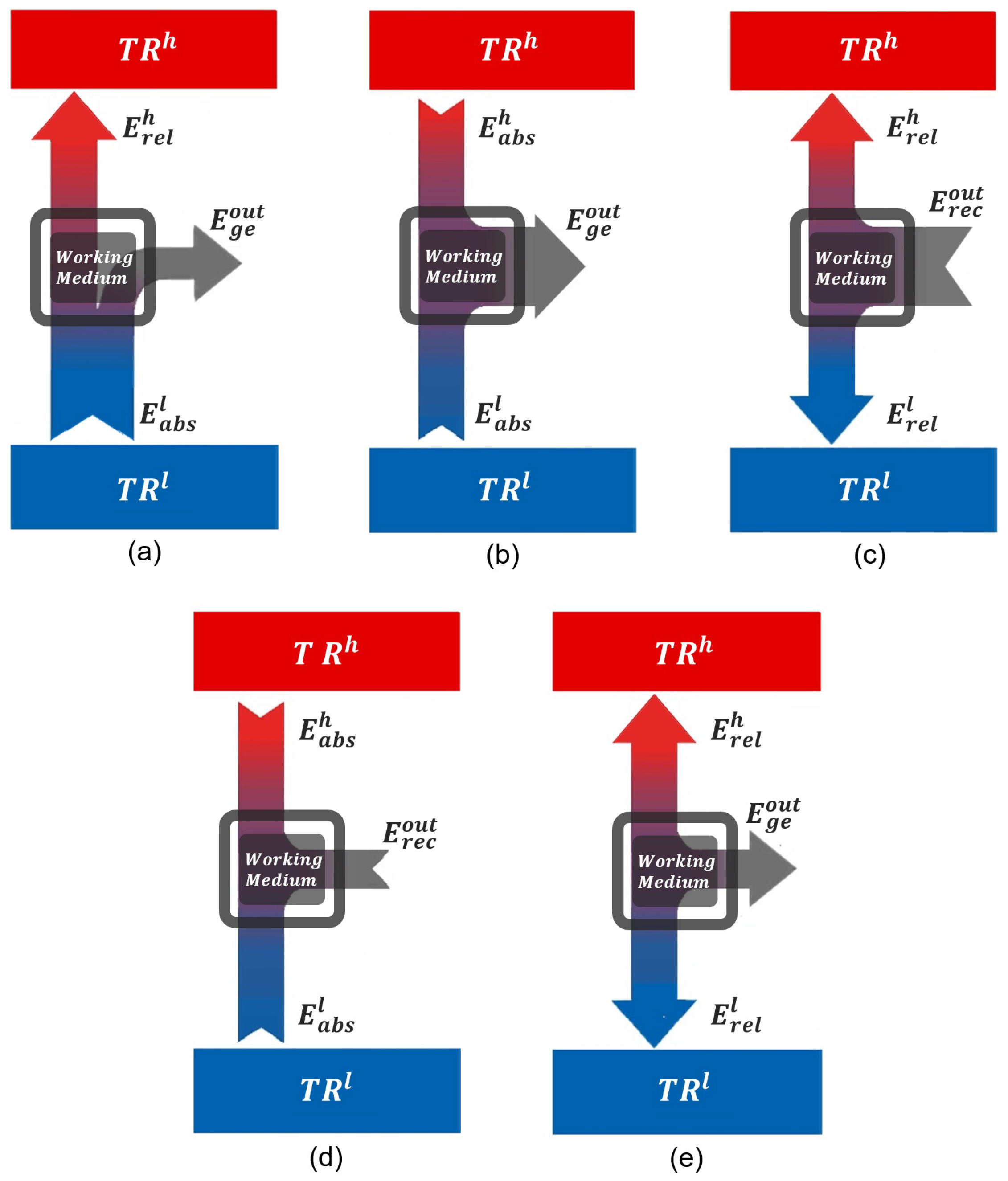
Appendix A.1. Violations of the Second Law

Figure A1a–c represent configurations that contradict the second law of thermodynamics, whether in the Clausius or Kelvin–Planck formulations.
(a)
The system absorbs energy E a b s l from the cold reservoir ( T R l ) and releases energy E r e l h to the hot reservoir ( T R h ) while simultaneously generating energy E g e o u t to the external environment. This configuration leads to a spontaneous transfer of energy from cold to hot, coupled with external energy generation, without any external compensation—a direct violation of the Clausius statement of the second law.
(b)
In this case, the system absorbs energy from both reservoirs ( E a b s h and E a b s l ) and generates E g e o u t to the external environment without releasing any energy back to either reservoir. This process violates the Kelvin–Planck statement by proposing the full conversion of thermal energy into external energy, which is thermodynamically impossible for any machine operating between two reservoirs.
(c)
The system releases energy to both reservoirs ( E r e l h and E r e l l ) while simultaneously receiving energy E r e c o u t from the external environment. This scenario is analogous to a device that, powered solely by external energy, heats both reservoirs—including the hot one—without generating entropy or any other compensating mechanism. Such a cyclic process is thermodynamically forbidden.

Appendix A.2. Violations of the First Law

Figure A1d,e clearly violate the first law of thermodynamics, which is the thermodynamic formulation of the conservation of energy.
(d)
The system absorbs energy E a b s h from T R h , E a b s l from T R l , and simultaneously receives E r e c o u t from the external environment. However, it does not release any energy to balance the total input, resulting in a clear violation of energy conservation.
(e)
The system releases energy E r e l h to T R h , E r e l l to T R l , and simultaneously generates E g e o u t to the external environment without receiving any incoming energy. This also constitutes a direct violation of the first law.
In summary, among the eight conceivable configurations for a system operating between T R h and T R l , only three satisfy both the first and second laws of thermodynamics and thus represent physically admissible thermal machine designs, as discussed in the main text. The remaining five configurations, illustrated in Figure A1, are thermodynamically forbidden and do not define any valid operational regime for a thermal machine.

References

  1. Thermodynamics in the Quantum Regime: Fundamental Aspects and New Directions, 1st ed.; Binder, F., Correa, L.A., Gogolin, C., Anders, J., Adesso, G., Eds.; Springer: Cham, Switzerland, 2018. [Google Scholar]
  2. Dann, R.; Kosloff, R. Unification of the first law of quantum thermodynamics. New J. Phys. 2023, 25, 043019. [Google Scholar] [CrossRef]
  3. Adlam, E.; Uribarri, L.; Allen, N. Symmetry and control in thermodynamics. AVS Quantum Sci. 2022, 4, 022001. [Google Scholar] [CrossRef]
  4. Aw, C.C.; Buscemi, F.; Scarani, V. Fluctuation theorems with retrodiction rather than reverse processes. AVS Quantum Sci. 2021, 3, 045601. [Google Scholar] [CrossRef]
  5. Goold, J.; Modi, K. Fluctuation theorem for nonunital dynamics. AVS Quantum Sci. 2021, 3, 045001. [Google Scholar] [CrossRef]
  6. Elouard, C.; Jordan, A.N. Efficient Quantum Measurement Engines. Phys. Rev. Lett. 2018, 120, 260601. [Google Scholar] [CrossRef]
  7. Kurizki, G.; Meher, N.; Opatrný, T. Nonlinearity and quantumness in thermodynamics: From principles to technologies. APL Quantum 2025, 2, 010901. [Google Scholar] [CrossRef]
  8. Medina-Dozal, L.; Urzúa, A.R.; Aranda-Lozano, D.; González-Gutiérrez, C.A.; Récamier, J.; Román-Ancheyta, R. Spectral response of a nonlinear Jaynes-Cummings model. Phys. Rev. A 2024, 110, 043703. [Google Scholar] [CrossRef]
  9. Khoudiri, A.; El Allati, A.; Müstecaplıoğlu, Ö.E.; El Anouz, K. Non-Markovianity and a generalized Landauer bound for a minimal quantum autonomous thermal machine with a work qubit. Phys. Rev. E 2025, 111, 044124. [Google Scholar] [CrossRef]
  10. Xia, S.; Lv, M.; Pan, Y.; Chen, J.; Su, S. Performance improvement of a fractional quantum Stirling heat engine. J. Appl. Phys. 2024, 135, 034302. [Google Scholar] [CrossRef]
  11. Deng, G.-X.; Ai, H.; Wang, B.; Shao, W.; Liu, Y.; Cui, Z. Exploring the Optimal Cycle for a Quantum Heat Engine Using Reinforcement Learning. Phys. Rev. A 2024, 109, 022246. [Google Scholar] [CrossRef]
  12. Williamson, L.A.; Davis, M.J. Many-Body Enhancement in a Spin-Chain Quantum Heat Engine. Phys. Rev. B 2024, 109, 024310. [Google Scholar] [CrossRef]
  13. Yuan, Y.Y.; Gu, Q. The Quantum Carnot-Like Heat Engine: The Level Degenerate Case. Int. J. Mod. Phys. B 2024, 38, 2450408. [Google Scholar] [CrossRef]
  14. Trushechkin, A.S.; Merkli, M.; Cresser, J.D.; Anders, J. Open quantum system dynamics and the mean force Gibbs state. AVS Quantum Sci. 2022, 4, 012301. [Google Scholar] [CrossRef]
  15. Khan, K.; Magalhães, W.F.; Araújo, J.S.; Bernardo, B.L.; Aguilar, G.H. Quantum Coherence and the Principle of Microscopic Reversibility. Phys. Rev. A 2023, 108, 052215. [Google Scholar] [CrossRef]
  16. Andrade, J.d.; Silva, Â.F.d.; Bernardo, B.d. Shortcuts to Adiabatic Population Inversion via Time-Rescaling: Stability and Thermodynamic Cost. Sci. Rep. 2022, 12, 11538. [Google Scholar]
  17. Vinjanampathy, S.; Anders, J. Quantum Thermodynamics. Contemp. Phys. 2016, 57, 545–579. [Google Scholar] [CrossRef]
  18. Myers, N.M.; Abah, O.; Deffner, S. Quantum thermodynamic devices: From theoretical proposals to experimental reality. AVS Quantum Sci. 2022, 4, 027101. [Google Scholar] [CrossRef]
  19. Scovil, H.E.D.; Schulz-DuBois, E.O. Three-Level Masers as Heat Engines. Phys. Rev. Lett. 1959, 2, 262. [Google Scholar] [CrossRef]
  20. Kieu, T.D. The Second Law, Maxwell’s Demon, and Work Derivable from Quantum Heat Engines. Phys. Rev. Lett. 2004, 93, 140403. [Google Scholar] [CrossRef]
  21. Quan, H.T.; Liu, Y.; Sun, C.P.; Noril, F. Quantum thermodynamic cycles and quantum heat engines. Phys. Rev. E 2007, 76, 031105. [Google Scholar] [CrossRef]
  22. Gelbwaser-Klimovsky, D.; Bylinskii, A.; Gangloff, D.; Islam, R.; Aspuru-Guzik, A.; Vuletic, V. Single-Atom Heat Machines Enabled by Energy Quantization. Phys. Rev. Lett. 2018, 120, 170601. [Google Scholar] [CrossRef] [PubMed]
  23. Zheng, Y.; Poletti, D. Work and efficiency of quantum Otto cycles in power-law trapping potentials. Phys. Rev. E 2014, 90, 012145. [Google Scholar] [CrossRef] [PubMed]
  24. Torrontegui, E.; Lizuain, I.; González-Resines, S.; Tobalina, A.; Ruschhaupt, A.; Kosloff, R.; Muga, J.G. Energy consumption for shortcuts to adiabaticity. Phys. Rev. A 2017, 96, 022133. [Google Scholar] [CrossRef]
  25. Uzdin, R.; Kosloff, R. The multilevel four-stroke swap engine and its environment. New J. Phys. 2014, 16, 095003. [Google Scholar] [CrossRef]
  26. Huang, X.L.; Xu, H.; Niu, X.Y.; Fu, Y.D. A special entangled quantum heat engine based on the two-qubit Heisenberg XX model. Phys. Scr. 2013, 88, 065008. [Google Scholar] [CrossRef]
  27. Wang, J.; He, J.; Mao, Z. Performance of a quantum heat engine cycle working with harmonic oscillator systems. Sci. China Phys. Mech. Astron. 2007, 50, 163. [Google Scholar] [CrossRef]
  28. Lin, B.; Chen, J. Optimization on the performance of a harmonic quantum Brayton heat engine. J. Appl. Phys. 2003, 94, 6185. [Google Scholar] [CrossRef]
  29. Filgueiras, C. Quantum heat machines enabled by the electronic effective mass. Results Phys. 2019, 15, 102556. [Google Scholar] [CrossRef]
  30. Khlifi, Y.; Allati, A.E.; Salah, A.; Hassouni, Y. Quantum heat engine based on spin isotropic Heisenberg models with Dzyaloshinskii–Moriya interaction. Int. J. Mod. Phys. B 2020, 34, 2050212. [Google Scholar] [CrossRef]
  31. Hawary, K.E.; Baz, M.E. Performance of an XXX Heisenberg model-based quantum heat engine and tripartite entanglement. Quantum Inf. Process. 2023, 22, 190. [Google Scholar] [CrossRef]
  32. Kosloff, R.; Rezek, Y. The Quantum Harmonic Otto Cycle. Entropy 2017, 19, 136. [Google Scholar] [CrossRef]
  33. Ivanchenko, E.A. Quantum Otto Cycle Efficiency on Coupled Qudits. Phys. Rev. E 2015, 92, 032124. [Google Scholar] [CrossRef] [PubMed]
  34. Fernando, L.F.C.; Cunha, M.M.; Silva, E.O. 1D Quantum ring: A Toy Model Describing Noninertial Effects on Electronic States, Persistent Current and Magnetization. Few Body Syst. 2022, 63, 58. [Google Scholar]
  35. Viefers, S.; Koskinen, P.; Deo, P.S.; Manninen, M. Quantum rings for beginners: Energy spectra and persistent currents. Physica E 2004, 21, 1. [Google Scholar] [CrossRef]
  36. Bartolo, B.D. Optical Interactions in Solids; Wiley: New York, NY, USA, 1991. [Google Scholar]
  37. De Assis, R.J.; Sales, J.S.; da Cunha, J.A.R.; Almeida, N.G.d. Universal two-level quantum Otto machine under a squeezed reservoir. Phys. Rev. E 2020, 102, 032111. [Google Scholar] [CrossRef]
  38. Chand, S.; Biswas, A. Measurement-induced operation of two-ion quantum heat machines. Phys. Rev. E 2017, 95, 032111. [Google Scholar] [CrossRef]
  39. Abd-Rabbou, M.Y.; Rahman, A.U.; Yurischev, M.A.; Haddadi, S. Comparative Study of Quantum Otto and Carnot Engines Powered by a Spin Working Substance. Phys. Rev. E 2023, 108, 034106. [Google Scholar] [CrossRef]
  40. Prakash, A.; Kumar, A.; Benjamin, C. Impurity reveals distinct operational phases in quantum thermodynamic cycles. Phys. Rev. E 2022, 106, 054112. [Google Scholar] [CrossRef]
  41. Vieira, C.H.S.; de Oliveira, J.L.D.; Santos, J.F.G.; Dieguez, P.R.; Serra, R.M. Exploring Quantum Thermodynamics with NMR. J. Magn. Reson. Open 2023, 16–17, 100105. [Google Scholar] [CrossRef]
  42. Kourkinejat, S.; Mahdifar, A.; Amooghorban, E. Quantum Otto engines with curvature-dependent efficiency: An analog model approach. Physica A 2025, 669, 130600. [Google Scholar] [CrossRef]
  43. Alsulami, M.D.; Abd-Rabbou, M.Y. Quantum Heat Engines with Spin-Chain-Star Systems. Ann. Phys. 2024, 536, 2400122. [Google Scholar] [CrossRef]
  44. De Oliveira, J.L.D.; Rojas, M.; Filgueiras, C. Two coupled double quantum-dot systems as a working substance for heat machines. Phys. Rev. E 2021, 104, 014149. [Google Scholar] [CrossRef] [PubMed]
  45. Filgueiras, C.; Rojas, M.; Silva, O.E.; Romero, C. Quantum heat machines enabled by twisted geometry. Int. J. Geom. Methods Mod. Phys. 2023, 20, 2450009. [Google Scholar] [CrossRef]
  46. Wu, Q.; Ciampini, M.A.; Paternostro, M.; Carlesso, M. Quantifying protocol efficiency: A thermodynamic figure of merit for classical and quantum state-transfer protocols. Phys. Rev. Res. 2023, 5, 023117. [Google Scholar] [CrossRef]
  47. Ali, M.M.; Huang, W.M.; Zhang, W.M. Quantum thermodynamics of single particle systems. Sci. Rep. 2020, 10, 13500. [Google Scholar] [CrossRef]
  48. Bernardo, B.L. Unraveling the role of coherence in the first law of quantum thermodynamics. Phys. Rev. E 2020, 102, 062152. [Google Scholar] [CrossRef]
  49. Li, C.-X. Protecting the Quantum Coherence of Two Atoms Inside an Optical Cavity by Quantum Feedback Control Combined with Noise-Assisted Preparation. Photonics 2024, 11, 400. [Google Scholar] [CrossRef]
  50. Ozaydin, F.; Sarkar, R.; Bayrakci, V.; Bayındır, C.; Altintas, A.A.; Müstecaplıoğlu, Ö.E. Engineering Four-Qubit Fuel States for Protecting Quantum Thermalization Machine from Decoherence. Information 2024, 15, 35. [Google Scholar] [CrossRef]
  51. Hamedani Raja, S.; Maniscalco, S.; Paraoanu, G.S.; Pekola, J.P.; Lo Gullo, N. Finite-Time Quantum Stirling Heat Engine. New J. Phys. 2021, 23, 033034. [Google Scholar] [CrossRef]
Figure 1. (a) General schematic of a QTM that consists of a quantum system as the working medium and two reservoirs T R h and T R l . The function of the working medium is to promote the exchange of energy between the TRs themselves as well as between the TRs and the QTM’s outside environment. (b) QTMs operating within the 2Acquirers’OR receive E r e c o u t from outside, absorb E a b s h from T R h , and release E r e l l to T R l . The 2Acquirers’OR includes two subregions: 2Acqout, where QTMs utilize E r e c o u t as their primary energy source, such as QCO and QHT; and 2Acqh, where QTMs utilize E a b s h as their primary energy source, such as QDP and QHO. (c) QTMs operating within the OutTransfers’OR absorb E a b s h from T R h , generate E g e o u t to outside, and release E r e l l to T R l . This operational region includes QEN and QLL. (d) QTMs operating within the Pumpers’OR absorb E a b s l from T R l , receive E r e c o u t from outside, and release E r e l h to T R h . This operational region includes QRE and QHP.
Quantumrep 07 00026 g001
Figure 2. Representation of the Carnot cycle in a T-S diagram for each operational region. The I–II-III–IV notation represents the thermodynamic states of the working medium and the cycle direction. This notation serves as the standard for all analyses in this study. T h and T l represent the maximum and minimum temperatures reached by the QTMs during the cycle, corresponding to the temperatures of T R h and T R l , respectively. (a) Counterclockwise Carnot cycle for QTMs in the 2Acquirers’OR. (b) Clockwise Carnot cycle for QTMs in the OutTransfers’OR. (c) Counterclockwise Carnot cycle for QTMs in the Pumpers’OR.
Quantumrep 07 00026 g002
Figure 3. Configurations of a two-level quantum system used as a working medium in its three distinct operational regions: (a) 2Acquirers’OR, (b) OutTransfers’OR, and (c) Pumpers’OR. The I–II-III–IV notation represents the thermodynamic states of the working medium and the cycle direction. For each configuration, there are four strokes, transitioning the system through four distinct states. E g l and E e l represent the ground and excited energy eigenvalues of the two-level quantum system, respectively, with an energy gap Δ l , while E g h and E e h denote the ground and excited levels for an energy gap Δ h . The strokes involve energy exchanges with the TRs—absorbing or releasing E γ h to/from T R h and E γ l to/from T R l —as well as changes in the system’s dimensional configuration, during which it either receives or delivers E o u t .
Quantumrep 07 00026 g003
Figure 4. Schematic representation of a maser or laser as a QEN based on the three-level model proposed by Scovil and Schultz-DuBois. The idler mode at frequency ω i connects to T R l , the pump at ω p connects to T R h . The signal at ω s (laser light) is interpreted as work generation. Energy levels | 1 , | 2 , and | 3 denote the quantum states involved in the lasing process.
Quantumrep 07 00026 g004
Figure 5. (a) A laser modeled as a quantum system with two two-level atoms labeled as A and B. The energy generated in ExT is interpreted as E g e o u t , and the laser light as E γ l released to T R l . (b) Laser viewed as a QTM operating in the OutTransfers’OR, as shown in the Figure 3d.
Quantumrep 07 00026 g005
Figure 6. E γ h (red squares), E γ l (blue circles), and E o u t (gray solid line) as functions of ρ , normalized by the maximum energy value, for e in a quantum ring as the working medium of QTMs operating in the Otto cycle, assuming T l = 1 K , θ 2 = 5 , and r l = 100 nm . The attached table provides the corresponding energy values, assisting in determining whether the energies are positive—indicating absorption (for TRs) or generation (for QTM’s outside)—or negative—indicating release (for TRs) or reception (from QTM’s outside). Solid vertical lines mark the boundaries between the operational regions, and the dashed line indicates the subregion division within the 2Acquirers’OR.
Quantumrep 07 00026 g006
Figure 7. Efficiencies as a function of ρ for all QTMs based on the e in a quantum ring operating in the Otto cycle. The graph was constructed using data from Table 2. The divisions, indicated by solid vertical lines, and the subdivision, indicated by a dashed vertical line, correspond to those in Figure 6. The minimum of ε QLL and the maximum of any other ε QTM occur at the intersection between the efficiency curve of each QTM and the dashed horizontal line, representing the ε QTM c of the corresponding QTM. Curve extensions beyond the permitted limits are omitted.
Quantumrep 07 00026 g007
Table 1. Summary of operational regions and their corresponding potential QTMs: essential information for any QTM using a working medium operating between T R h and T R l governed by principles analogous to those applied in this work.
OR
α 2 Range
α 2 = E h E l
QTM ε QTM ε QTM Limit
θ 2 = T h T l
ε QTM
Relationship
α 2 LimitOR
Intersection
α 2 Value
Bi-Acquirers
“2Acquirers”
0 < α 2 < 1
2 Acq o u t Quantum Cooler
QCO
ε QCO = E a b s h E r e c o u t = α 2 1 α 2 ε QCO c = 1 θ 2 1
ε QCO max = ε QCO c α 2 1
ε QHT ε QCO = 1
ε QHT > ε QCO
α QCO min 2 = 0
α QCO max 2 = 1 θ 2
Quantum Heater
QHT
ε QHT = E r e l l E r e c o u t = 1 1 α 2 ε QHT c = θ 2 θ 2 1
ε QHT max = ε QHT c α 2 1
α QHT min 2 = 0
α QHT max 2 = 1 θ 2
α 2 Acq o u t 2 Acq h 2 = 1 θ 2
2 Acq h Quantum Thermal
Damper
QDP
ε QDP = E r e c o u t E a b s h = 1 α 2 α 2 ε QDP c = θ 2 1
ε QDP max = ε QDP c α 2 0
ε QHO ε QDP = 1
ε QHO > ε QDP
α QDP min 2 = 1 θ 2
α QDP max 2 = 1
Quantum Heating
Optimizer
QHO
ε QHO = E r e l l E a b s h = 1 α 2 ε QHO c = θ 2
ε QHO max = ε QHO c α 2 0
α QHO min 2 = 1 θ 2
α QHO max 2 = 1
α 2 Acq OutT 2 = 1
Outside Transfers
“OutTransfers”
α 2 > 1
Quantum Thermal
Laser-Like
QLL
ε QLL = E r e l l E a b s h = 1 α 2 ε QLL c = 1 θ 2
ε QLL min = ε QLL c α 2
ε QEN + ε QLL = 1
ε QEN < 1
ε QLL < 1
α QEN min 2 = 1
α QEN max 2 = θ 2
Quantum Thermal
Engine
QEN
ε QEN = E g e o u t E a b s h = α 2 1 α 2 ε QEN c = θ 2 1 θ 2
ε QEN max = ε QEN c α 2
α QLL min 2 = 1
α QLL max 2 = θ 2
α OutT Pump 2 = θ 2
Thermal Pumpers
“Pumpers”
α 2 > 1
Quantum
Refrigerator
QRE
ε QRE = E a b s l E r e c o u t = 1 α 2 1 ε QRE c = 1 θ 2 1
ε QRE max = ε QRE c α 2 1
ε QHP ε QRE = 1
ε QHP > ε QRE
α QRE min 2 = θ 2
α QRE max 2
Quantum Heat
Pumper
QHP
ε QHP = E r e l h E r e c o u t = α 2 α 2 1 ε QHP c = θ 2 θ 2 1
ε QHP max = ε QHP α 2 1
α QHP min 2 = θ 2
α QHP max 2
Table 2. Summary of operational regions of e in a quantum ring as the working medium acting between T R h and T R l and their corresponding potential QTMs operating in the Otto cycle. Results obtained from the expressions summarized in Table 1 for θ 2 = 5 and ρ = α , where ρ = r l / r h [Equation (100)].
OR
ρ = α
QTM ε QTM ε QTM Limit
θ 2 = 5
ρ LimitOR Intersection
ρ Value
2Acquirers
0 < ρ 2 < 1
2 Acq o u t  QCO   ε QCO = ρ 2 1 ρ 2   ε QCO max = ε QCO c = 0.25   ρ QCO min = 0
ρ QCO max = 0.45  
QHT ε QHT = 1 1 ρ 2 ε QHT max = ε QHT c = 1.25 ρ QHT min = 0
ρ QHT max = 0.45
ρ 2 Acq o u t 2 Acq h = 0.45
2 Acq h QDP ε QDP = 1 ρ 2 ρ 2 ε QDP max = ε QDP c = 4 ρ QDP min = 0.45
ρ QDP max = 1
QHO ε QHO = 1 ρ 2 ε QHO max = ε QHO c = 5 ρ QHO min = 0.45
ρ QHO max = 1
ρ 2 Acq OutT = 1
OutTransfers
ρ 2 > 1
QLL ε QLL = 1 ρ 2 ε QLL min = ε QLL = 0.20 ρ QEN min = 1
ρ QEN max = 2.24
QEN ε QEN = ρ 2 1 ρ 2 ε QEN max = ε QEN c = 0.80 ρ QLL min = 1
ρ QLL max = 2.24
ρ OutT Pump = 2.24
Pumpers
ρ 2 > 1
QRE ε QRE = 1 ρ 2 1 ε QRE max = ε QRE c = 0.25 ρ QRE min = 2.24
ρ QRE max
QHP ε QHP = ρ 2 ρ 2 1 ε QHP max = ε QHP = 1.25 ρ QHP min = 2.24
ρ QHP max
Disclaimer/Publisher’s Note: The statements, opinions and data contained in all publications are solely those of the individual author(s) and contributor(s) and not of MDPI and/or the editor(s). MDPI and/or the editor(s) disclaim responsibility for any injury to people or property resulting from any ideas, methods, instructions or products referred to in the content.

