Article

Uncertainty Relation and the Thermal Properties of an Isotropic Harmonic Oscillator (IHO) with the Inverse Quadratic (IQ) Potentials and the Pseudo-Harmonic (PH) with the Inverse Quadratic (IQ) Potentials

1
Department of Physics, Kogi State University, Anyigba 272102, Nigeria
2
Theoretical Physics Group, Department of Physics, University of Uyo, Uyo 520003, Nigeria
3
Department of Physics, University of Port Harcourt, Choba 500004, Nigeria
*
Author to whom correspondence should be addressed.
Quantum Rep. 2023, 5(1), 38-51; https://doi.org/10.3390/quantum5010004
Submission received: 15 December 2022 / Revised: 31 December 2022 / Accepted: 5 January 2023 / Published: 12 January 2023
(This article belongs to the Topic Theoretical, Quantum and Computational Chemistry)

Abstract

:
The solutions for a combination of the isotropic harmonic oscillator plus the inversely quadratic potentials and a combination of the pseudo-harmonic with inversely quadratic potentials has not been reported, though the individual potentials have been given attention. This study focuses on the solutions of the combination of the potentials, as stated above using the parametric Nikiforov–Uvarov (PNV) as the traditional technique to obtain the energy equations and their corresponding unnormalized radial wave functions. To deduce the application of these potentials, the expectation values, the uncertainty in the position and momentum, and the thermodynamic properties, such as the mean energy, entropy, heat capacity, and the free mean energy, are also calculated via the partition function. The result shows that the spectra for the PHIQ are higher than the spectra for the IHOIQ. It is also shown that the product of the uncertainties obeyed the Heisenberg uncertainty relation/principle. Finally, the thermal properties of the two potentials exhibit similar behaviours.

1. Introduction

The reliability of numerical techniques is a fact, but the analytical methods are less time-consuming and less complicated, there are few potential functions that can be admitted via an approximation scheme. The exact solutions of the different quantum potential terms, such as the Manning–Rosen potential [1], Rosen–Morse potential [2], Morse potential [3], Pöschl–Teller potential [4], Coulomb potential [5], Yukawa potential [6], Hellmann potential [7], Harmonic potential [8], and others, in the recent time, have attracted a lot of attention because they contain the necessary information to study quantum models, and they also justify the correctness of the quantum theory. The solutions are valuable results that check and improve the models, as well as the numerical methods formulated to solve the complicated physical systems. The most frequently used traditional techniques are the Nikiforov–Uvarov method [9], asymptotic iteration method [10,11], supersymmetry quantum mechanics [12,13], factorization method [14], 1/N shifted expansion method [15], the supersymmetric WKB method [16], the exact and proper quantization rule [17], the formula method for bound state problems [18], etc. In most cases, the solutions obtained are the eigenvalues and eigenfunctions for both the relativistic and nonrelativistic regimes. It is noted that in early quantum mechanics, there are a limited number of exactly solvable problems. There are other reports on the Schrödinger equation [19,20]. Recently, efforts have been devoted to the exactly solvable problems. The solvable problems can be classified as exactly solvable potentials that determine the full spectrum, analytically, for a continuous range of values of the potential parameters. The second solvable problem is the conditionally exactly solvable potentials with solutions that can only be generated for the specific values of the potential parameters. However, the analytic exact solutions of some of these exponential-type potentials (ETPs), such as the Yukawa potential, Hellmann potential, and Frost Musulin potential, are impossible for any = 0 state. Therefore, to obtain the solution to such a system, the use of an approximation scheme to deal with the centrifugal barrier is inevitable. Motivated by the interest in the non-ETPs, the present work examines the influence of the potential parameters on the energy of a system and some expectation values for a combination of the isotropic harmonic oscillator (IHO) and the inversely quadratic (IQ) potential as well as a combination of the pseudo-harmonic (PH) potential with the inversely quadratic (IQ) potential. The combination of the potentials to be studied in this work are given by
V I H O I Q ( r ) = m ω 2 r 2 2 + D 0 r 2 ,
V P H I Q ( r ) = D e r 2 r e 2 + D e r e 2 + D 0 r 2 2 D e ,
where ω = 2 π f ,   m is the mass of a string, f is the frequency of the vibration, D 0 is a potential strength, r e is the equilibrium bond separation and D e is the dissociation energy.

2. Methodology

In this study, the method of the parametric Nikiforov–Uvarov is applied. According to Tezcan and Sever [21,22], a general form of the equation
d 2 ψ ( s ) d s 2 + w 1 w 2 s s ( 1 w 3 s ) d ψ ( s ) d s + p 0 s 2 + p 1 s p 2 s 2 ( 1 w 3 s ) 2 ψ ( s ) = 0 ,
is useful in this method. Using Equation (3), the authors give the condition for the energy equation and its corresponding wave function as
w 2 n ( 2 n + 1 ) w 5 + + 2 w 3 w 8 + ( 2 n + 1 + 2 w 8 ) w 9 = n ( 1 n ) w 3 w 7 ( 2 n + 1 ) w 3 w 8 ,
ψ ( s ) = N s w 12 ( 1 w 3 s ) w 12 w 13 w 3 P n ( w 10 1 , w 11 w 3 w 10 1 ) ( 2 w 3 s ) .
The values of the parametric constants in Equations (4) and (5) are obtained, as follows:
w 4 = 0.5 ( 1 w 1 ) , w 5 = 0.5 ( w 2 2 w 3 ) , w 6 = w 5 2 + p 0 , w 7 = 2 w 4 w 5 p 1 , w 8 = w 4 2 + p 2 , w 9 = w 3 ( w 7 + w 3 w 8 ) + w 6 , w 10 = 2 ( w 4 + w 8 + 1 2 ) , w 11 = w 2 2 ( w 5 w 9 w 3 w 8 ) , w 12 = w 4 + w 8 , w 13 = w 5 w 9 w 3 w 8 } .

3. Bound State Solutions

To solve any quantum system for a given potential function, the Schrödinger equation for a three-dimensional system containing the potential model is given as
p 2 2 μ ψ n , , m ( r ) = ( E n , V ( r ) ) ψ n , , m ( r ) ,
where E n , is the non-relativistic energy of the system, μ is the reduced mass of a particle, V ( r ) is the interacting potential, and ψ n , , m ( r ) is the total wave function. Setting the total wave function ψ n , , m ( r ) = R n , ( r ) Y , m ( θ , ϕ ) r 1 , the radial Schrödinger equation is obtained as
d 2 R n , ( r ) d r 2 + 2 μ 2 [ E n , V ( r ) V c e n ( r ) ] R n , ( r ) = 0 .
The V c e n ( r ) in Equation (8) is a centrifugal potential given by the formula
V c e n ( r ) = ( + 1 ) 2 2 μ r 2 .
Plugging Equations (1) and (9) into the radial equation of Equation (8) and then, using a transformation y = r 2 , Equation (8) becomes
d 2 R n , ( y ) d y 2 + 1 2 y d R n , ( y ) d y + μ m π 2 f 2 y 2 2 + μ E n , y 2 2 μ D 0 2 2 ( + 1 ) 4 y 2 R n , ( y ) = 0 ,
Comparing Equation (10) with Equation (3), the parameters in Equation (6) have their respective values as
w 1 = 1 2 , w 2 = w 3 = 0 , w 4 = 1 4 , w 5 = 0 , w 6 = μ m π 2 f 2 2 , w 7 = μ E n , 2 2 , w 8 = 1 16 + μ D 0 2 2 + ( + 1 ) 4 , w 9 = μ m π 2 f 2 2 , w 10 = 1 + 1 2 ( 1 + 2 ) 2 + 8 μ D 0 2 , w 11 = 2 μ m π 2 f 2 2 , w 12 = 1 4 + 1 4 ( 1 + 2 ) 2 + 8 μ D 0 2 , w 13 = μ m π 2 f 2 2 } .
Substituting the correct parametric constants in Equation (11) into Equations (4) and (5), respectively, the solutions for the IHOIQ potential are given as
E n , = 2 μ [ μ m π 2 f 2 ( 2 n + 1 + 1 2 ( 1 + 2 ) 2 + 8 μ D 0 2 ) ] ,
R n , ( y ) = y 1 4 + 1 16 + μ D 0 2 2 + ( + 1 ) 4 e μ D 0 2 2 + μ m π 2 f 2 2 y L n 2 1 16 + μ D 0 2 2 + ( + 1 ) 4 ( 2 μ D 0 2 2 + μ m π 2 f 2 2 y ) .
Using the PHIQ potential given in Equation (2), and follow the same procedures to obtain Equation (12), we have the energy equation for the PHIQ potential as
E n , = 2 μ [ μ D e 2 r e 2 ( 2 n + 1 + 1 2 ( 1 + 2 ) 2 + 8 μ ( D e r e 2 + D 0 ) 2 ) μ D e ] .

4. Expectation Values

Here, we obtained the expectation values via the Hellmann Feynman theory. According to this theorem [23,24], when the spatial distribution of the electrons has been determined by solving the Schrödinger equation, then, all forces in the system can be calculated through classical electrostatics. If the Hamiltonian H for a particular quantum system is a function of some parameters q , with the eigenvalues and eigenfunctions of H , respectively, given by E n , ( q ) and R n , ( q ) , theoretically, then, we can write
E q q = ψ q | H q q | ψ q ,
with the effective Hamiltonian of the potential as
H I H O I Q = 2 2 μ d 2 d r 2 + 2 2 μ ( + 1 ) r 2 + m ω 2 r 2 2 + D 0 r 2 ,
H P H I Q = 2 2 μ d 2 d r 2 + 2 2 μ ( + 1 ) r 2 + D e r 2 r e 2 + D e r e 2 + D 0 r 2 2 D e ,
we can obtain the expectation values. Setting q = D 0 , q = m , and q = , for H I H O I Q , we have the following expectation values
p 2 = 4 π f μ m ( 1 + 2 ) 2 + 8 μ D 0 2 .
r 2 = ( 2 n + 1 + 1 2 ( 1 + 2 ) 2 + 8 μ D 0 2 ) 2 π f μ m .
r 2 = 2 π f μ m ( 1 + 2 ) 2 + 8 μ D 0 2 .
Setting q = μ , and q = D e , for H P H I Q , Oyewumi and Sen [25] have the following expectation values
p 2 = 2 μ D e 2 2 μ D e r e 2 ( 2 n + 1 + 1 2 ( 1 + 2 ) 2 + 8 μ ( D e r e 2 + D 0 ) 2 ) 4 μ D e ( 1 + 2 ) 2 + 8 μ ( D e r e 2 + D 0 ) 2 2 μ D e r e 2 2 ,
r 2 = 2 r e 2 2 μ D e ( 2 n + 1 + 1 2 ( 1 + 2 ) 2 + 8 μ ( D e r e 2 + D 0 ) 2 ) .

Thermodynamic Properties

In this section, we calculate the thermodynamic properties of both potential (1) and potential (2). To do this, first, the energy equation in Equations (12) and (14), respectively, are written in the form
E n l = ( 4 n Q 1 + 2 Q 1 + Q 1 Q 2 )
E n l = 4 n Ω 1 + ( 2 Ω 1 + Ω 2 )
where
Q 1 = μ m π 2 f 2 μ , Q 2 = ( 1 + 2 l ) 2 + 8 μ D 0 2 , Ω 1 = μ μ D e 2 r e 2 , Ω 2 μ μ D e 2 r e 2 ( 1 + 2 l ) 2 + 8 μ ( D e r e 2 + D 0 ) 2 D e r e } .
The partition function is defined as
Z ( β ) = 0 λ e β E n d n
Substituting Equation (23) for Equation (26), the partition function is given as
Z ( β ) = e β ( 2 Q 1 + Q 1 Q 2 ) 0 λ e 4 β n Q 1 d n
Using Maple version 10.0, the partition function is evaluated as
Z ( β ) = e 4 λ β Q 1 e β ( 2 Q 1 + Q 1 Q 2 ) 4 β Q 1
Other thermodynamic properties can be obtained using the partition function.
(a)
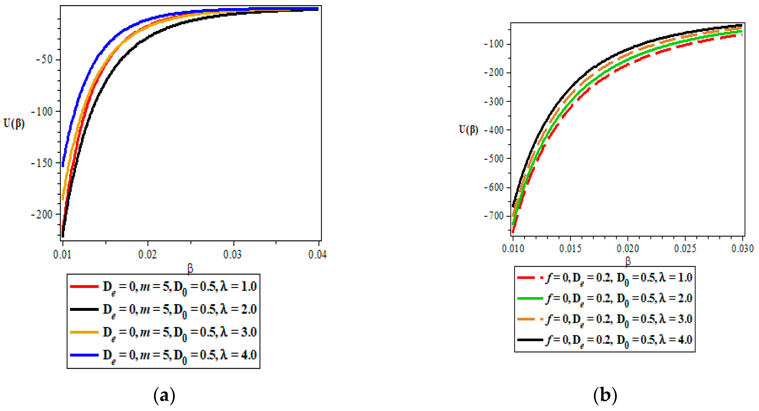
Vibrational mean energy.
The vibrational mean energy is given as
U ( β ) = ln Z ( β ) β = { e β Q 1 ( 2 + Q 2 + 4 λ ) ( 2 β Q 1 + β Q 1 Q 2 + 4 λ β Q 1 + 1 ) 4 β 2 Q 1 } .
(b)
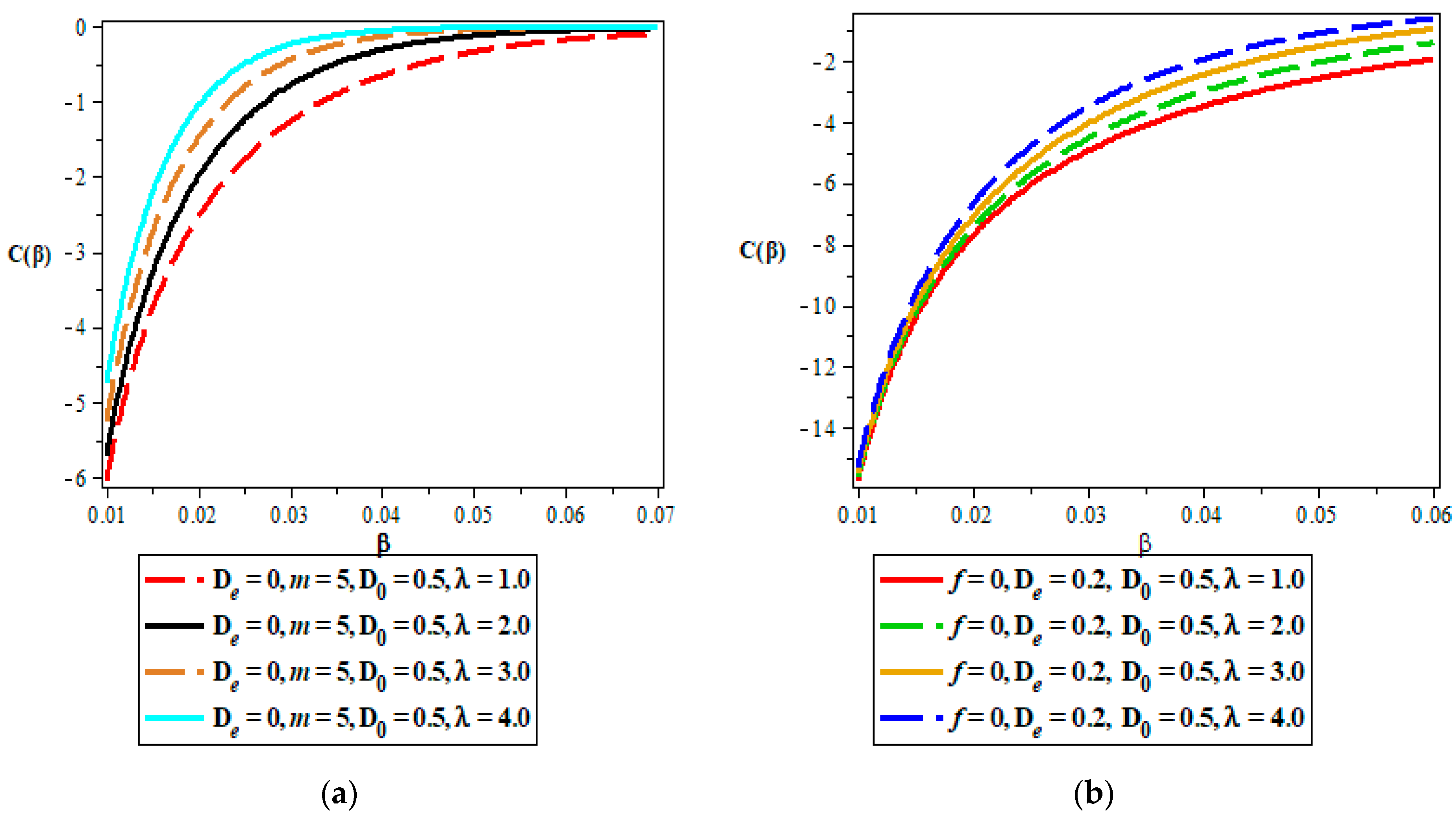
Vibrational heat capacity.
The vibrational heat capacity is given as
C ( β ) = k β 2 2 ln Z ( β ) β 2 = k { e β Q 1 ( 2 + Q 2 + 4 λ ) ( 4 β 2 Q 1 2 + 4 β 2 Q 1 2 Q 2 + 16 β 2 Q 1 2 λ + 4 β Q 1 + β 2 Q 1 2 Q 2 2 + 8 β 2 Q 1 2 Q 2 λ + 2 β Q 1 Q 2 + 16 β 2 Q 1 2 λ 2 + 8 λ β Q 1 + 2 ) 4 β Q 1 } .
(c)
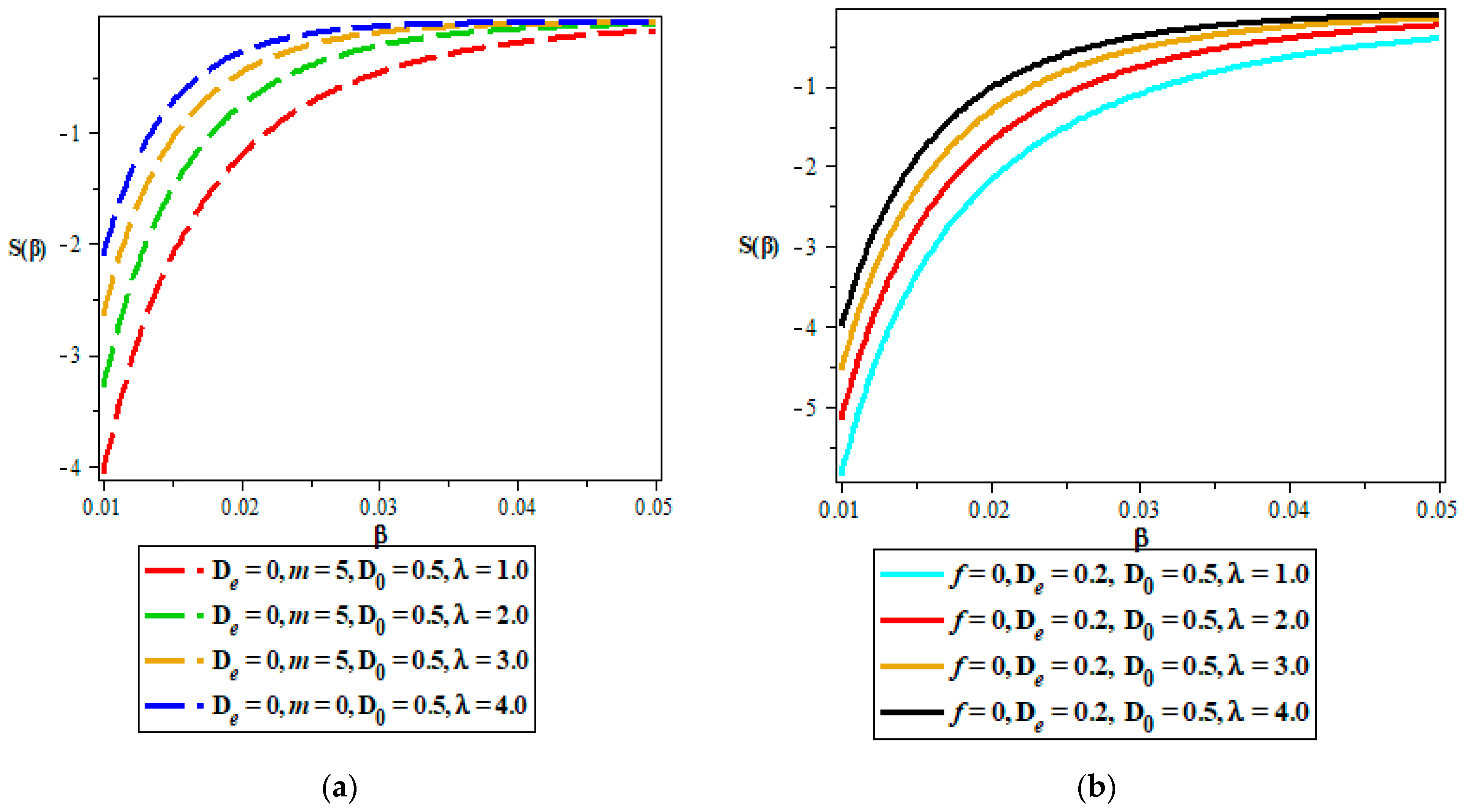
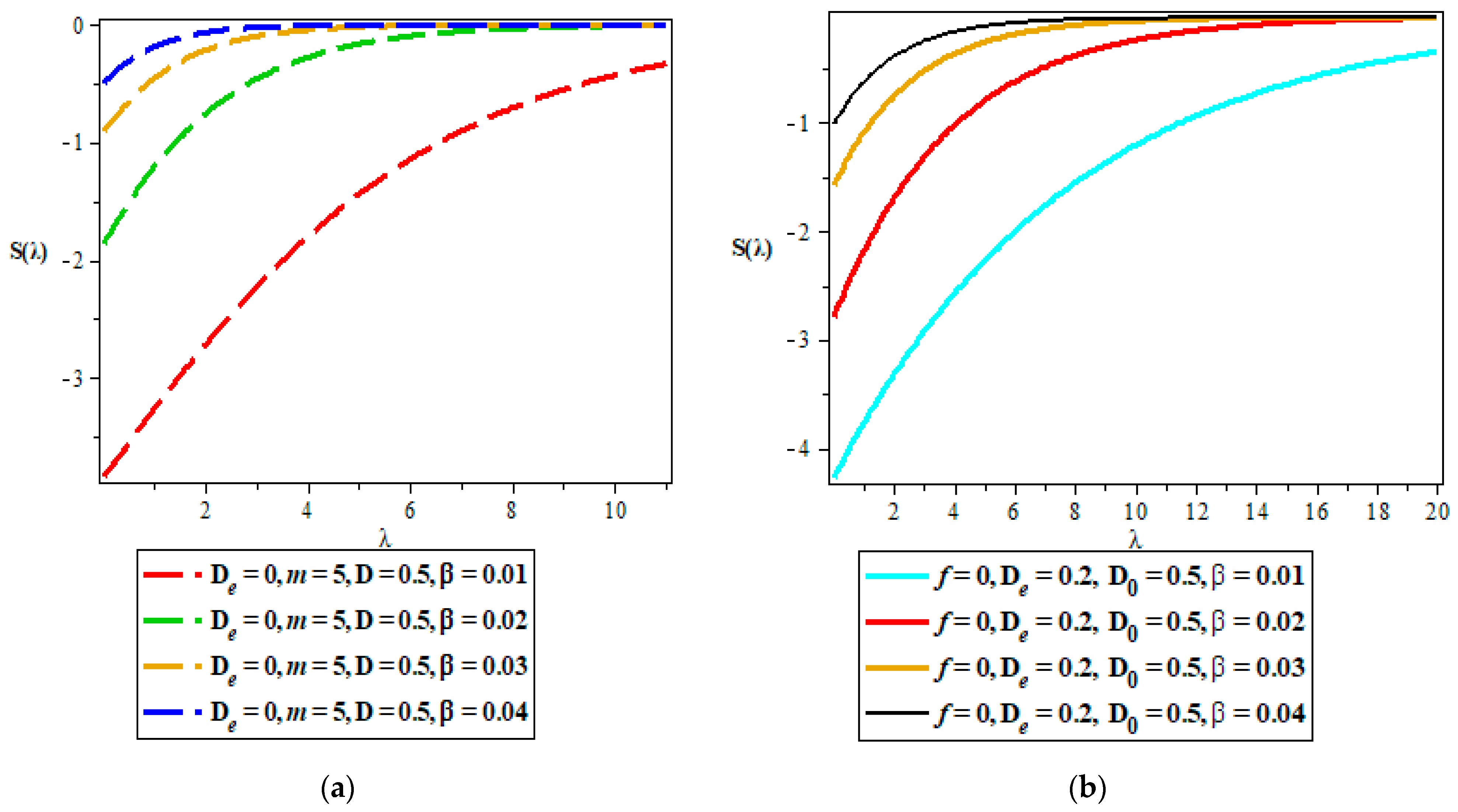
Vibrational entropy.
The vibrational entropy is given as
S ( β ) = k ln Z ( β ) k β ln Z ( β ) β = k ln { e 4 λ β Q 1 e β ( 2 Q 1 + Q 1 Q 2 ) 4 β Q 1 } k β { e β Q 1 ( 2 + Q 2 + 4 λ ) ( 2 β Q 1 + β Q 1 Q 2 + 4 λ β Q 1 + 1 ) 4 β 2 Q 1 } } .
(d)
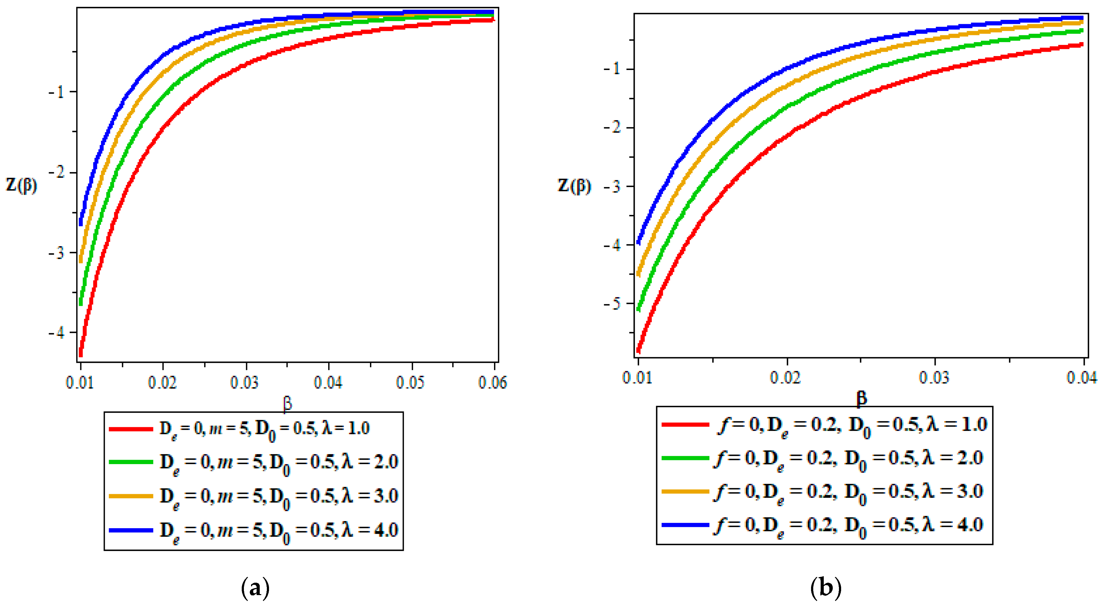
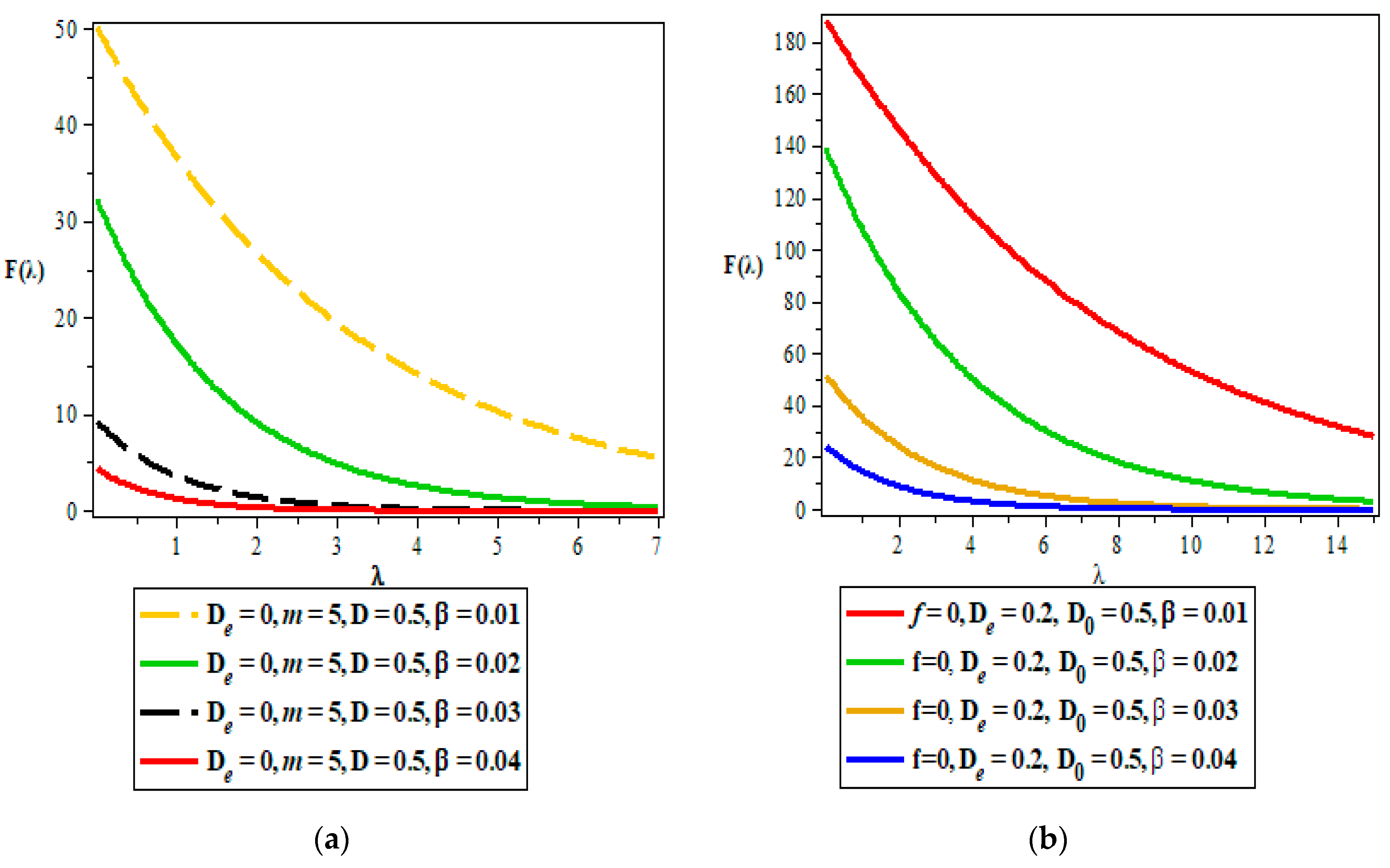
Vibrational Free energy
The vibrational free energy is given as
F ( β ) = 1 β ln Z ( β ) = 1 β ln ( e 4 λ β Q 1 e β ( 2 Q 1 + Q 1 Q 2 ) 4 β Q 1 )

5. Discussion

In Table 1, the energy eigenvalues for the two different values of the angular momentum were presented for various quantum states. A linear variation is observed between the quantum state and the energy eigenvalues for the two categories of the potentials. The same trend was also observed between the energy eigenvalue and the angular momentum. The energy eigenvalues of the IHOIQ potential for the ground state and the first excited state with two values of the strength of the IQ potential for the various masses, are presented in Table 2. A linear variation between the mass of the spring and the energy eigenvalues is observed. It has been shown, from the Table 2, that the result of the ground state of the IHO potential with D 0 = 3 , is the same as the result of the first excited state of the IHO for the different masses of the spring. The momentum and position expectation values, the uncertainty, and the product of the expectations, as well as the product of the uncertainty of the IHOIQ potential, are presented in Table 3 and Table 4. The frequency varies directly with the momentum expectation value, as well as with the uncertainty in the momentum, but inversely with the position expectation value and the uncertainty in the position. The same variation is observed against the mass of the spring in Table 4. The results from Table 3 and Table 4 showed that the product of the expectation of the momentum and the position at any frequency or mass is a constant. This was also noticed in the product of the uncertainty. The results of the uncertainty showed that the more precisely a system is measured, the less precisely the other can be measured. This aligned with the Heisenberg uncertainty product given as
Δ p Δ r 2 .
It is noted that the expectation values in Equations (18) and (20) have a relation of the form
p 2 = 2 r 2 .
In Table 5 and Table 6, the momentum and the position expectation values, the uncertainty and the product of the expectations, as well as the product of the uncertainty of the PHIQ potential, are presented for the various dissociation energy and equilibrium lengths, respectively. The results obtained in Table 3 and Table 4 are equally obtained in Table 5. However, the variation of the equilibrium bond length against the expectation values, the uncertainty and their product, are the inverse of what is obtained in Table 3, Table 4 and Table 5. In all cases, the uncertainty product obeys the standard Heisenberg uncertainty relation.
Figure 1, Figure 2, Figure 3, Figure 4, Figure 5, Figure 6, Figure 7, Figure 8, Figure 9 and Figure 10 showed the thermodynamic properties of the PHIQ and IHOIQ potentials for the various upper bound and temperature parameters. The figures in (a) are the thermal properties for the IHOIQ potential while the figures in (b) are the thermal properties for the IHOIQ potential. The variation of Z(ꞵ) against ꞵ for the different λ is presented in Figure 1. Z(ꞵ) rises as ꞵ increases and tends to converge at a higher ꞵ. It shows that as the temperature of the system becomes lower, Z(ꞵ) for the various λ, compact together. In Figure 2, the variation of U(ꞵ) against ꞵ for different λ, is shown. U(ꞵ) varies inversely with the temperature of the system. At every given temperature, the vibrational U(ꞵ) of the IHOIQ potential are higher than the vibrational U(ꞵ) of the PHIQ potential. The mean energy tends to converge as the temperature becomes lower. The convergence is more obvious in the IHOIQ potential than in the PHIQ potential at higher temperatures. C(ꞵ) and ꞵ vary directly with one another, as shown in Figure 3. C(ꞵ) at the different λ, converged at the origin for the two potential systems, and diverged as ꞵ increased. The divergence becomes greater for the PHIQ potential as ꞵ remains on the increase, but for the IHOIQ potential, C(ꞵ) converged. Figure 4 presents the vibrational S(ꞵ) against ꞵ for the various λ. The same behaviour was observed in Figure 1 and is also observed here. Thus, the effect of ꞵ on S(ꞵ) and Z(ꞵ) are the same. Figure 5 shows the variation of the vibrational F(ꞵ) against ꞵ for the different λ. The vibrational F(ꞵ) decreases monotonically as ꞵ increases. As the temperature of the system lowers, F(ꞵ) becomes smaller and tends to converge. The vibrational Z(λ) against λ for the various ꞵ, is shown in Figure 6. As λ increases, Z(λ) also increases. Z(λ) of the two potentials for the different ꞵ, are the same. Figure 7 shows the vibrational U(λ) against λ for the various ꞵ. U(λ) rises and tends to converge as λ increases. A slight difference is observed in the two potential systems. Figure 8 presents the variation of the vibrational C(λ) against λ for the different ꞵ. The effect seen in Figure 7 is also obtained in Figure 8. The variation of the vibrational S(λ) against λ for the different ꞵ, is shown in Figure 9. The effect observed in Figure 6 is also observed in Figure 9. The variation of the vibrational F(λ) against λ for the different ꞵ, is shown in Figure 10. The vibrational F(λ) decreases exponentially while λ increases linearly. The vibrational F(λ) for the highest ꞵ in the IHOIQ potential corresponds to the vibrational F(λ) for the lowest ꞵ in the PHIQ potential.

6. Conclusions

The result of the Schrödinger equation for the IHOIQ (isotropic harmonic oscillator with inversely quadratic) potential and the PHIQ (pseudoharmonic with inversely quadratic) potential has been obtained via a simplified traditional method. It has been shown that the result of the IHOIQ (isotropic harmonic oscillator with inversely quadratic) at the ground state, is the same as the result of the IHO for the first excited state. It was also shown that the spectra obtained for the IHOIQ (isotropic harmonic oscillator with inversely quadratic) are lesser than the spectra obtained for the PHIQ (pseudoharmonic with inversely quadratic). The product of the uncertainty obtained for the two potential models obeyed the Heisenberg uncertainty inequality. Finally, the thermal properties for the two potential models showed similar features.

Author Contributions

Formulation of the work: C.A.O.; Calculations: C.A.O. and I.B.O.; Introduction: M.C.O.; Editing: A.D.A.; Numerical results/Plotting: I.B.O. and C.A.O.; Discussion of the results: G.O.J. All authors have read and agreed to the published version of the manuscript.

Funding

This research received no external funding.

Institutional Review Board Statement

Not applicable.

Informed Consent Statement

Not applicable.

Data Availability Statement

The data used in the study are in the text.

Conflicts of Interest

The authors declare no conflict of interest.

References

  1. Zhang, M.-C.; An, B. Analytical Solutions of the Manning-Rosen Potential In the Tridiagonal Program. Chin. Phys. Lett. 2010, 27, 110301. [Google Scholar]
  2. Oyewumi, K.J.; Akosile, C.O. Bound state solutions of the Dirac-Rosen-Morse potential with spin and pseudospin symmetry. Eur. Phys. J. A 2010, 45, 311–318. [Google Scholar] [CrossRef] [Green Version]
  3. Miraboutalebi, S.; Rajae, L. Solutions of N-dimensional Schrödinger equation with Morse potential via Laplace transforms. J. Math. Chem. 2014, 52, 1119–1128. [Google Scholar] [CrossRef]
  4. Jia, C.-S.; Zhang, L.-H.; Pen, X.-L. Improved Poschl-Teller potential energy model for diatomic molecules. Int. J. Quantum Chem. 2017, 2017, e25383. [Google Scholar] [CrossRef]
  5. Antia, A.D.; Ituen, E.E.; Obong, H.P.; Isonguyo, C.N. Analytical solutions of the modified Coulomb potential using the factorization method. Int. J. Recent Adv. Phys. 2015, 4, 55–65. [Google Scholar] [CrossRef]
  6. Napsuciale, M.; Rodriguez, S. Complete analytical solution to the quantum Yukawa potential. Phys. Lett. B 2021, 816, 136218. [Google Scholar] [CrossRef]
  7. Onate, C.A.; Onyeaju, M.C.; Ikot, A.N.; Ebomwonyi, O. Eigen solutions and entropic system for Hellmann potential in the presence of the Schrodinger equation. Eur. Phys. J. Plus 2017, 132, 462. [Google Scholar] [CrossRef]
  8. Antia, A.D.; Eze, C.C.; Akpabio, L.E. Solutions of the Schrödinger equation with the harmonic oscillator potential (HOP) in cylindrical basis. Phys. Astron. Int. J. 2018, 2, 187–191. [Google Scholar] [CrossRef]
  9. Ghanbari, A.; Khordad, R.; Taghizadeh, F. Influence of Coulomb term on thermal properties of fluorine. Chem. Phys. Lett. 2022, 801, 139725. [Google Scholar] [CrossRef]
  10. Bayrak, O.; Boztosun, I. Bound state solutions of the Hulthẻn potential by using the asymptotic iteration method. Phys. Scr. 2007, 76, 92–96. [Google Scholar] [CrossRef]
  11. Falaye, B.J.; Oyewumi, K.J.; Ikhdair, S.M.; Hamzavi, M. Eigensolution techniques, their applications and Fisherʼs information entropy of the Tietz–Wei diatomic molecular model. Phys. Scr. 2014, 89, 115204. [Google Scholar] [CrossRef]
  12. Wei, G.-F.; Dong, S.-H. Pseudospin symmetry in the relativistic Manning-Rosen potential including a Pekeris-type approximation to the pseudo-centrifugal term. Phys. Lett. B 2010, 686, 288–292. [Google Scholar] [CrossRef] [Green Version]
  13. Onate, C.A.; Onyeaju, M.C. Fisher information of a vector potential for time-dependent Feinberg–Horodecki equation. Int. J. Quantum Chem. 2020, 2020, e26543. [Google Scholar] [CrossRef]
  14. Onyeaju, M.C.; Idiodi, J.; Ikot, A.; Solaimani, M.; Hassanabadi, H. Linear and nonlinear optical properties in spherical quantum dots: Generalized Hulthén potential. Few-Body Syst. 2016, 57, 793–805. [Google Scholar] [CrossRef]
  15. Mustafa, O.; Sever, R. Approach to the shifted 1/N expansion for the Klein-Gordon equation. Phys. Rev. A 1991, 43, 5787. [Google Scholar] [CrossRef]
  16. Omugbe, E.; Osafile, O.E.; Okon, I.B.; Eyube, E.S.; Inyang, E.P.; Okorie, U.S.; Jahanshir, A.; Onate, C.A. Non-relativistic bound state solutions with α-deformed Kratzer-type potential using the super-symmetric WKB method: Application to theoretic-information measures. Eur. Phys. J. D 2022, 76, 72. [Google Scholar] [CrossRef]
  17. Gu, X.-Y.; Dong, S.-H.; Ma, Z.-Q. Energy spectra for modified Rosen-Morse potential solved by the exact quantization rule. J. Phys. A Math. Theor. 2009, 42, 035303. [Google Scholar] [CrossRef]
  18. Falaye, B.J.; Ikhdair, S.M.; Hamzavi, M. Formula method for bound state problems. Few-Body Syst. 2015, 56, 63–78. [Google Scholar] [CrossRef] [Green Version]
  19. Uddin, M.F.; Hafez, M.G.; Hammouch, Z.; Bileanu, D. Periodic and rogue waves for Heisenberg models of ferromagnetic spin chains with fractional beta derivative evolution and obliqueness. Waves Random Complex Media 2021, 31, 2135–2149. [Google Scholar] [CrossRef]
  20. Xie, J.; Zhang, Z. An effective dissipation-preserving fourth-order difference solver for fractional-in-space nonlinear wave equations. J. Sci. Comput. 2019, 79, 1753–1776. [Google Scholar] [CrossRef]
  21. Tezcan, C.; Sever, R. A General Approach for the Exact Solution of the Schrödinger equation. Int. J. Theor. Phys. 2009, 48, 337–350. [Google Scholar] [CrossRef]
  22. Njoku, I.J.; Onyenegecha, C.P.; Okereke, C.J.; Opara, A.I.; Ukewuihe, U.M.; Nwaneho, F.U. Approximate solutions of Schrodinger equation and thermodynamic properties with Hua potential. Results Phys. 2021, 24, 104208. [Google Scholar] [CrossRef]
  23. Feynman, R.P. Forces in Molecules. Phys. Rev. 1039, 56, 340. [Google Scholar] [CrossRef]
  24. Barut, A.O.; Inomata, A.; Wilson, R. A new realization of dynamical groups and factorisation method. J. Phys. A Math. Gen. 1987, 20, 4075. [Google Scholar] [CrossRef]
  25. Oyewumi, K.J.; Sen, K.D. Exact solutions of the Schrödinger equation for the pseudoharmonic potential: An application to some diatomic molecules. J. Math Chem. 2012, 50, 1039–1059. [Google Scholar] [CrossRef]
Figure 1. (a,b) Vibrational partition function against the temperature parameter for the IHOIQ potential and the PHIQ potential, respectively. The vibrational partition function increases as the temperature parameter increases for the two interacting potentials. The IHOIQ converges more as the temperature parameter increases. It shows that as the temperature of the system becomes lower, Z(ꞵ) for the various λ, compact together.
Quantumrep 05 00004 g001
Figure 2. (a,b) Vibrational mean energy against the temperature parameter for the IHOIQ potential and the PHIQ potential, respectively. The vibrational mean energy varies directly with the temperature parameter for both IHOIQ and PHIQ potentials with IHOIQ having the more convergence at higher values of the temperature parameter. At every given temperature, the vibrational U(ꞵ) of the IHOIQ potential are higher than the vibrational U(ꞵ) of the PHIQ potential.
Quantumrep 05 00004 g002
Figure 3. (a,b) Vibrational heat capacity against the temperature parameter for the PH with the IQ potentials and the IHO with the IQ potentials, respectively. The vibrational heat capacity rises as the temperature parameter increases. The heat capacity for PHIQ diverges while that of IHOIQ converges as the temperature parameter rises. The divergence becomes greater for the PHIQ potential as ꞵ remains on the increase, but for the IHOIQ potential, C(ꞵ) converged.
Quantumrep 05 00004 g003
Figure 4. (a,b) Vibrational entropy against the temperature parameter for the IHOIQ potential and the PHIQ potential, respectively. The vibrational entropy varies directly with the temperature parameter. The entropy at various upper bound converges as the temperature parameter rises. Thus, the effect of ꞵ on S(ꞵ) and Z(ꞵ) are the same.
Quantumrep 05 00004 g004
Figure 5. (a,b) Vibrational free energy against the temperature parameter for the IHOIQ potential and the PHIQ potential, respectively. The vibrational free energy decreases monotonically while the temperature parameter increases linearly.
Quantumrep 05 00004 g005
Figure 6. (a,b) Vibrational partition function against the upper bound for the IHOIQ potential and the PHIQ potential, respectively. The partition function for IHOIQ and PHIQ have the same behviour for various temperature parameter.
Quantumrep 05 00004 g006
Figure 7. (a,b) Vibrational mean energy against the upper bound for the IHOIQ potential and the PHIQ potential, respectively. The mean energy varies directly with the upper bound for different values of the temperature parameter. A slight difference is observed in the two potential systems.
Quantumrep 05 00004 g007
Figure 8. (a,b) Vibrational heat capacity against the upper bound for the IHOIQ potential and the PHIQ potential, respectively. The heat capacity increases with the upper bound for both potentials.
Quantumrep 05 00004 g008
Figure 9. (a,b) Vibrational entropy against the upper bound for the PH with the IQ potentials and the IHO with the IQ potentials, respectively. The entropy varies directly with the upper bound but converges at higher values of the upper bound.
Quantumrep 05 00004 g009
Figure 10. (a,b) Vibrational free energy against the upper bound for the PH with the IQ potentials and the IHO with the IQ potentials, respectively. The vibrational free energy decreases monotonically as the upper bound increases gradually. The vibrational F(λ) for the highest ꞵ in the IHOIQ potential corresponds to the vibrational F(λ) for the lowest ꞵ in the PHIQ potential.
Quantumrep 05 00004 g010
Table 1. Energy eigenvalues of the IHOIQ potential and the PHIQ potential with μ = = m = f = 1 and r e = 0.1 .
n IHOIQ   ( D 0 = 5 ) PHIQ   ( D e = D 0 = 1 )
= 0 = 1 = 0 = 1
026.40981928.28571433.449411041.3654140
138.98124840.85714361.733683069.6496850
251.55267653.42857190.017954097.9339570
364.12410566.000000118.302225126.218228
476.69553378.571429146.586496154.502499
589.26696291.142857174.870768182.786770
6101.83839103.71429203.155039211.071042
7114.40982116.28571231.439310239.355313
8126.98125128.85714259.723581267.639584
9139.55268141.42857288.007853295.923855
Table 2. Energy eigenvalues of the IHOIQ potential with μ = = = m = f = 1 .
m n = 0 n = 1
D 0 = 0 D 0 = 3 D 0 = 0 D 0 = 3
19.42857122.0000022.0000034.57143
213.3340131.1127031.1127048.89138
316.3307738.1051238.1051259.87947
418.8571444.0000044.0000069.14286
521.0829349.1935049.1935077.30406
623.0951953.8887753.8887784.68236
724.9456658.2065358.2065391.46740
826.6680362.2254062.2254097.78277
928.2857166.0000066.00000103.7143
Table 3. Expectation values and uncertainty in the position and the momentum of the IHOIQ potential with μ = = = m = 1 and D 0 = 5 for the various frequencies.
f p 2 r 2 Δ p Δ r p 2 r 2 Δ p Δ r
11.7959180.7159091.3401190.8461141.2857141.133893
23.5918370.3579551.8952140.5982931.2857141.133893
35.3877550.2386362.3211540.4885041.2857141.133893
47.1836730.1789772.6802380.4230571.2857141.133893
58.9795920.1431822.9965970.3783941.2857141.133893
610.775510.1193183.2826070.3454251.2857141.133893
712.571430.1022733.5456210.3198011.2857141.133893
814.367350.0894893.7904280.2991471.2857141.133893
916.163270.0795454.0203560.2820381.2857141.133893
Table 4. Expectation values and the uncertainty in the position and momentum of the IHOIQ potential with μ = = = f = 1 and D 0 = 5 for the various masses.
m p 2 r 2 Δ p Δ r p 2 r 2 Δ p Δ r
11.7959180.7159091.3401190.8461141.2857141.133893
22.5398120.5062241.5936790.7114941.2857141.133893
33.1106220.4133301.7636960.6429081.2857141.133893
43.5918370.3579551.8952140.5982931.2857141.133893
54.0157960.3201642.0039450.5658311.2857141.133893
64.3990840.2922692.0973990.5406191.2857141.133893
74.7515530.2705882.1798060.5201811.2857141.133893
85.0796240.2531122.2538020.5031021.2857141.133893
95.3877550.2386362.3211540.4885041.2857141.133893
Table 5. Expectation values and the uncertainty in the position and momentum at the ground state of the PHIQ potential with μ = = = f = 1 and D 0 = 5 for the various masses.
D e p 2 r 2 Δ p Δ r p 2 r 2 Δ p Δ r
163.6685810.3184007.9792590.56426920.2720764.502452
290.0685530.2252859.4904450.47464220.2911374.504568
3110.334130.18406110.5040060.42902420.3082364.506466
4127.419680.15950211.2880330.39937820.3237494.508187
5142.468780.14275311.9360280.37782720.3378924.509755
6156.067540.13039712.4927000.36110620.3508144.511188
7168.563960.12080112.9832180.34756420.3626214.512496
8180.184620.11307013.4232870.33625820.3733994.513690
9191.086830.10667013.8234160.32660420.3832134.514777
Table 6. Expectation values and the uncertainty in the position and momentum at the ground state of the PHIQ potential with μ = = = f = 1 ,   r e = 0.1 and D e = D 0 = 5 for the various masses.
r e p 2 r 2 Δ p Δ r p 2 r 2 Δ p Δ r
1142.46880.14275311.936030.37782720.3378924.509755
270.922860.2881908.4215710.53683320.4392574.520980
346.283540.4388896.8032000.66248720.3133204.507030
433.027930.5972355.7469930.77281019.7254404.441333
524.105030.7653624.9096870.87485018.4490654.295237
617.210770.9451174.1485870.97217116.2662014.033138
711.393671.1380653.3754511.06680212.9667393.600936
86.2037331.3455022.4907291.1599588.34713702.889141
91.4083031.5684861.1867191.2523922.20890301.486238
Disclaimer/Publisher’s Note: The statements, opinions and data contained in all publications are solely those of the individual author(s) and contributor(s) and not of MDPI and/or the editor(s). MDPI and/or the editor(s) disclaim responsibility for any injury to people or property resulting from any ideas, methods, instructions or products referred to in the content.

