Article

Assessing the Precision of Quantum Simulation of Many-Body Effects in Atomic Systems Using the Variational Quantum Eigensolver Algorithm

1
Institute for Theoretical Physics, FAU Erlangen-Nurnberg, 91058 Erlangen, Germany
2
Centre for Quantum Engineering, Research and Education, TCG CREST, Salt Lake, Kolkata 700091, India
3
Department of Physics, Tokyo Institute of Technology, 2-12-1 Ookayama, Meguro-ku, Tokyo 152-8550, Japan
4
Atomic, Molecular and Optical Physics Division, Physical Research Laboratory, Navrangpura, Ahmedabad 380009, India
*
Author to whom correspondence should be addressed.
Quantum Rep. 2022, 4(2), 173-192; https://doi.org/10.3390/quantum4020012
Submission received: 5 March 2022 / Revised: 6 April 2022 / Accepted: 7 April 2022 / Published: 15 April 2022

Abstract

:
The emerging field of quantum simulation of many-body systems is widely recognized as a very important application of quantum computing. A crucial step towards its realization in the context of many-electron systems requires a rigorous quantum mechanical treatment of the different interactions. In this pilot study, we investigate the physical effects beyond the mean-field approximation, known as electron correlation, in the ground state energies of atomic systems using the classical-quantum hybrid variational quantum eigensolver algorithm. To this end, we consider three isoelectronic species, namely Be, Li , and B + . This unique choice spans three classes—a neutral atom, an anion, and a cation. We have employed the unitary coupled-cluster ansätz to perform a rigorous analysis of two very important factors that could affect the precision of the simulations of electron correlation effects within a basis, namely mapping and backend simulator. We carry out our all-electron calculations with four such basis sets. The results obtained are compared with those calculated by using the full configuration interaction, traditional coupled-cluster and the unitary coupled-cluster methods, on a classical computer, to assess the precision of our results. A salient feature of the study involves a detailed analysis to find the number of shots (the number of times a variational quantum eigensolver algorithm is repeated to build statistics) required for calculations with IBM Qiskit’s QASM simulator backend, which mimics an ideal quantum computer. When more qubits become available, our study will serve as among the first steps taken towards computing other properties of interest to various applications such as new physics beyond the Standard Model of elementary particles and atomic clocks using the variational quantum eigensolver algorithm.

1. Introduction

Recent advances in quantum information science and technology have heralded the second quantum revolution [1]. These developments have led to new pathways to tackle the challenging quantum many-body problem using quantum computers and simulators [1,2,3,4,5,6,7,8]. The interest in many-body aspects of electronic structure using quantum computers/simulators stems from the potential speed-up that a quantum computer promises to offer [9,10,11] over a classical computer in calculating properties such as energies. An overview of the developments in this field can be found in Ref. [2]. Among the algorithms that calculate the ground state energy of a quantum many-body system, approaches such as the quantum phase estimation algorithm [10,12] may produce energy estimates with high accuracy, but require long coherence times [13,14,15]. An alternative that promises to alleviate this problem, especially in the noisy-intermediate scale quantum era that we are now in, is the Variational Quantum Eigensolver algorithm [16,17]. The underlying principle of the variational quantum eigensolver is to minimize the ground state energy of a system through a quantum-classical hybrid approach by tuning the variational parameters in the appropriate quantum circuit. It has been experimentally realized in platforms such as photonic processors [17], superconducting qubits [18], ion traps [19], and so forth.
Precise quantum many-body calculations in atoms and molecules are based on a rigorous treatment of the electron correlation effects. Although simulations of electronic structures have been performed using quantum algorithms, not much emphasis has been placed on obtaining the correct correlation trends, mostly owing to the proof-of-principle nature of the calculations [20]. Moreover, energies of a whole host of molecular systems, such as H 2 O [21], H 2 [13,20] (also see Ref. [22] for an excited state treatment using an extended version of the variational quantum eigensolver), HeH + [17,23], LiH, BeH 2 [20], and H 4 [24], have been calculated, but atomic systems have received little attention, except for one work on H , which is a relatively simple system [25], despitefinding many applications [26,27,28,29,30,31,32]. Atomic systems, in our view, merit separate study, since they have been and are still being used in testing new physics, such as parity violation [28,30,33,34] and electric dipole moments of quarks [35,36]. Atoms can provide insights on a variety of physics problems such as those mentioned in the previous sentence, via many-body calculations of relevant properties (for example, see Ref. [37]). Atomic systems are still considered the most suitable candidates for making accurate clocks [38,39,40,41,42,43], probing nuclear structures by studying isotope shifts [44,45], investigating fundamental physics such as new physics beyond the standard model of particle physics by analysing atomic parity violation and precise values of g j factors [46], and many more. All these studies entail the performance of high-accuracy atomic calculations (even less than 1% level). Many such studies are performed in heavier atomic systems, for which quantum computers will be more appropriate than classical ones, when more qubits will be available in the future. At this point, we will comment on evaluating properties other than energy using the variational quantum eigensolver algorithm, and their importance when more qubits become available. The converged parameters from a variational quantum eigensolver calculation are used in constructing the wave function, which is used in calculating the energies. One then evaluates a property of interest with the converged amplitudes and appropriate property integrals. These include atomic properties of interest such as the hyperfine structure constants. With appropriate modifications, this approach can be used to calculate properties of interest to fundamental physics (such as probing the electric dipole moment of the electron), and properties such as dipole polarizabilities for atomic clocks. Atoms cannot be viewed as subsets of molecules, in that the correlation effects and trends in a molecule and its constituent atoms can be quite dissimilar. Atomic systems have shown to display their own unique features in this regard, in particular the conservation of orbital angular momentum in these systems [47]. Moreover, atoms are better platforms than molecules for testing the dependence of properties on the number of qubits, since the latter is composed of two or more atoms, and hence the required number of qubits, in general, grow much faster when one goes from lighter to heavier systems. In this work, we conduct a study on carefully chosen atomic systems, in which we strive to understand the precision with which the all-important electron correlation effects are captured by quantum simulations using the variational quantum eigensolver algorithm. Specifically, within a given basis set, we check with different combinations of fermionic to qubit operator mapping and backend simulator if our quantum simulation results lie within the neighborhood of the best possible result within that basis, thus setting a measure for the precision of our results. In summary, we study the trends in the ground state energies, and in particular the correlation part of the energies, of the chosen systems with respect to choice of bases, fermionic to qubit mapping schemes, and backends both within an atomic system and across the considered systems. In addition, we compare our results with those obtained from a traditional computation by using several many-body methods. Since this is the first study of this kind on atomic systems, we strongly believe that the results and conclusions from this work will pave the way for further works on atoms. This will be a new and refreshing addition to the otherwise common approach of going up in the length scale, from diatomics to polyatomics and aimed at eventually moving to drug design on complex molecules etc, to moving in the opposite direction to atomic systems, which we reiterate has somehow received little attention.
On physical grounds, many-body effects are expected to behave differently in ions and neutral atoms of isoelectronic systems. Among them, electron correlation effects in the negative ions are vastly different [48,49] owing to the short-range potentials that bind the outer valence electron in these ions [50]. Negative ions find several applications, which is evident from the sheer volume of literature on them [50,51,52]. Atomic calculations from earlier works have also shown that electron correlation effects in the alkaline earth-metal atoms are very prominent due to strong repulsion between the outer two valence electrons in these atoms [53,54,55]. For these reasons and keeping in mind the steep cost of simulation in the noisy-intermediate scale quantum era, we consider here isoelectronic neutral beryllium (Be), lithium anion (Li ), and boron cation (B + ) as representative systems to investigate roles of electron correlation effects in the determination of their ground state energies. We also stress on the fact that the study undertaken in this work is general in nature, and should be applicable to other heavier atomic systems in higher quality basis sets, when such simulations become feasible. It is also worth adding that the systems that have been investigated in this work find many applications. For example, light systems such as Be can serve as excellent systems in probing roles of different kinds of electromagnetic interactions [56,57], as well as obtaining nuclear charge radii from measurements of isotope shifts [58]. Moreover, Be is a very interesting system from a many-body theoretic viewpoint, as it is well known that its ground state has a multireference character [47]. Systems such as Li may find applications in plasma diagnostics [59]. Group IIIA ions have been known to hold great promise for atomic clocks [60]. Specifically, B + , holds promise, since the transition of interest has an extremely long lifetime in its excited state. Moreover, because the 10 B + ion’s mass is closer to that of 9 Be + , there would be efficient state exchange for quantum logic detection [61].
The accuracy of the calculated ground state energy of a system using a variational quantum eigensolver algorithm depends upon several factors, including the crucial aspect of choosing a variational form, as it dictates the form of the wave function. The other elements that need special attention are the choice of mapping technique used to convert the second quantized fermionic operators describing the Hamiltonian and wave function to their spin counterparts, the backend simulator for running quantum circuits, and the classical optimizer, besides the more intuitive and traditional features such as the choice of single-particle basis in the many-body calculations. We focus extensively on the required number of shots for obtaining reliable results using Qiskit’s QASM simulator backend. Employing the QASM simulator marks a significant departure from the otherwise common use of the statevector backend (for example, see Refs. [62,63,64,65]. Some works such as Ref. [66] use QASM, but with much fewer shots (4096) than possibly required). While both the backends are used for the same variational quantum eigensolver algorithm, the latter relies on matrix manipulations whereas the former is measurement-based. Our investigation is especially necessary, as it explicitly provides estimates for expected error from a measurement-based scheme. This sets the ground for future analyses where one may include noise models and error mitigation, which then would be more realistically comparable to a calculation performed on a real quantum computer.

2. Theory

2.1. The Variational Quantum Eigensolver Algorithm

The ground state energy functional of an atomic system within the classical-quantum hybrid variational quantum eigensolver algorithm is given as:
E 0 ( θ ) = Ψ 0 ( θ ) | H a | Ψ 0 ( θ ) Ψ 0 ( θ ) | Ψ 0 ( θ ) = Φ 0 | U ( θ ) H a U ( θ ) | Φ 0 ,
where | Ψ 0 ( θ ) is the trial wave function and H a is the atomic Hamiltonian. The former is parametrized as | Ψ 0 ( θ ) = U ( θ ) | Φ 0 , where the unitary operator, U ( θ ) , depends on a set of arbitrary parameters, denoted collectively as θ , and | Φ 0 is a suitable initial many-body wave function. For the choice of U ( θ ) , that is, the ansätz, we adopt the unitary coupled-cluster variational form. The initial state is constructed by employing the Hartree-Fock (HF) approximation. In this framework, the total Hamiltonian is expressed as H a = H 0 + V e s , constructed out of the effective one-body HF Hamiltonian H 0 and the residual interaction term V e s [47]. Therefore, the total energy is computed as E 0 = E H F + E c o r r with the HF energy E H F = Φ 0 | H a | Φ 0 and correlation energy E c o r r arising from the residual interaction V e s . The unitary coupled-cluster theory accounts for these correlation effects via an exponential ansätz acting on the HF wave function, with the exponent expressed as the sum of excitation operators. Further, in this ansätz, the Trotterization [67] procedure is used to decompose U ( θ ) into smaller operators to implement it efficiently in a quantum circuit. Throughout, we work with | Ψ 0 ( θ ) in its second quantized form, where the relevant mathematical structures are recast in the language of creation and annihilation operators. In Equation (1), the atomic Hamiltonian, H a , too is expressed in the second quantized form as
H a = p q D h p q a p a q + 1 2 p q r s D h p q r s a p a q a r a s ,
where h p q and h p q r s denote one-body and two-body integrals of H a , respectively, D refers to the number of spin-orbitals from the chosen single particle basis, and the notations { p , q , r , s } denote general atomic orbitals.
To compute atomic energies in the framework of quantum simulation, one needs to express the second quantized fermionic operators that occur in both the wave function as well as the Hamiltonian as spin operators that contain a sequence of unitary operations. We use three such mapping techniques, namely the Jordan–Wigner, Parity, and the Bravyi–Kitaev transformations. In the Jordan–Wigner transformation [68], one works in the occupation number basis. For a given site, k, the creation and annihilation operators, a k and a k , are related to their corresponding gate structures, A k and A k , via the Jordan–Wigner transformation, by
A k = j = 1 k 1 Z j Q k + j = k + 1 D I j ,
and
A k = j = 1 k 1 Z j Q k j = k + 1 D I j ,
where Q k + and Q k are given by:
Q k + = X k + ι ˙ Y k 2 ,
and
Q k = X k ι ˙ Y k 2 ,
D refers to the total number of qubits for the considered system, and X, Y, and Z are the Pauli operators/gates. The string j = 1 k 1 Z j in Equations (3) and (4) ensures that in the spin operator-transformed version, the required phase change that occurs when a creation or annihilation operator acts on an arbitrary Fock state is accounted for. In the case of atoms, this would correspond to D spin-orbitals, with N electrons, or in other words, N occupied and ( D N ) unoccupied spin-orbitals. Note that for the description of a given A k , one needs to take into account a tensor product of Z gates that contains ( k 1 ) terms. Therefore, when one constructs terms such as A i A j + A j A i , which one normally encounters in atomic calculations, the resulting term has tensor product of Pauli gates from index i through j, with all the in-between indices occurring in steps of one. Thus, the number of qubit operations for Jordan–Wigner transformation scales as O ( D ) . In case of parity transformation, the k t h qubit stores the parity of all the spin-orbitals up to k. Thus, parity transformation is known to work in the parity basis. The parity mapping uses two-qubit reduction arising from the Z 2 symmetry, thereby reducing the number of required qubits by two. We note that the parity transformation too scales as O ( D ) . The Bravyi–Kitaev transformation works in the Bravyi–Kitaev basis, which finds a golden mean by borrowing from both of above mentioned approaches, and leads to lesser number of required gates. The number of qubits scales as O ( l o g D ) . We have not provided the relevant equations for the parity and the Bravyi–Kitaev transformations as we have for the Jordan–Wigner mapping, and an interested reader can find a comprehensive discussion on all these three transformations in Refs. [68,69].
The circuits thus constructed by starting from Equation (1) are evaluated with an initial set of guess parameters in an appropriate backend simulator (either statevector or qiskit’s QASM backend), and the energy is obtained. The statevector simulator executes the set of circuits associated with a system without measurements or shots, given an input state vector. The QASM simulator mimics an ideal quantum computer, in that it gives probabilistic outcomes as counts for each of the states, after multiple shots. After evaluating Equation (1), we pass the energy to an optimizer, which runs on a classical computer. This module uses an optimization algorithm, and minimizes the energy, obtained from the previous step of the variational quantum eigensolver algorithm, with respect to the parameters. Once the new parameters are obtained, they are fed back as inputs to the quantum circuit from the previous step. This process is repeated until the energy is minimized. The energy thus obtained is guaranteed to be an upper bound to the true ground state energy.

2.2. Many-Body Methods

The ground state energy, E 0 , with the exact wave function | Ψ 0 of an atomic system can be determined by
E 0 = Ψ 0 | H a | Ψ 0 Ψ 0 | Ψ 0 .
The full configuration interaction (FCI) method can be employed to determine on | Ψ 0 exactly for a given basis set by expressing as
| Ψ 0 = C 0 | Φ 0 + C I | Φ I + C I I | Φ I I + + C N | Φ N ,
where { C } s are the expansion coefficients with the Slater determinants | Φ s generated by exciting the HF wave function | Φ 0 . Due to extremely steep computational cost, truncated configuration interaction (CI) method is usually considered in the multi-electron systems for practical scenarios. At a given level of truncation, the coupled-cluster theory accounts for electron correlation effects more rigorously and satisfies size-consistency and size-extensivity characteristics in contrast to the configuration interaction method, thereby earning the title of the gold standard of electronic structure calculations [70]. In the coupled-cluster theory ansätz, | Ψ 0 yields the exponential form as (e.g., see Refs. [70,71])
| Ψ 0 = e T | Φ 0 ,
where T = T 1 + T 2 + . . . + T N is a sum of excitation operators generating particle-hole excitations with the level denoted by subscript. The amplitudes of these operators are obtained on a classical computer by solving the following equation
Φ 0 K | H a | Φ 0 = 0 ,
where H a e T H a e T = H a e T l with subscript l representing the linked terms [70]. The K on the right hand side of the above equation denotes the K t h excitation out of the HF state. For example, in the CCSD method, there are two amplitude equations, one with K denoting single excitations, and the other with K specifying double excitations. Once the amplitudes associated with the T operators (t-amplitudes) are obtained, the energy of the system is calculated by:
E 0 = Φ 0 | H a | Φ 0 Φ 0 | e T H a e T | Φ 0 ,
where the inequality sign indicates that the energy expression given by Equation (11) is not variational in an approximated coupled-cluster theory owing to non-hermitian property of H a , but it terminates naturally.
It is desirable to work with unitary operators in the framework of quantum computation/simulation. For this purpose, we take recourse to the unitary coupled-cluster theory over the coupled-cluster theory. In the approximated unitary coupled-cluster theory framework [72], U ( θ ) = e Θ ( θ ) with Θ ( θ ) = T T such that t-amplitudes are used as θ . One can immediately see from the above equation that the unitary coupled-cluster operator involves not only the excitation operator T but also the de-excitation operator T . The energy expression follows:
E 0 = Φ 0 | e Θ H a e Θ | Φ 0 = Φ 0 | e Θ H a e Θ | Φ 0 = Φ 0 | e T T H a e T T | Φ 0 .
Unlike in the traditional version of the coupled-cluster method, e T T H a e T T does not terminate naturally in the above equation, but it guarantees that the energy thus calculated obeys the variational principle. Owing to the non-terminating form, Equation (12) cannot be evaluated efficiently in the traditional unitary coupled-cluster method on a classical computer without resorting to brute-force termination of the expression. However, this issue is circumvented on a quantum computer/simulator.
To carry out the analysis conveniently, we have used the approximated coupled-cluster theory to singles and doubles approximation (CCSD method). The singles and doubles approximated unitary coupled-cluster theory is henceforth mentioned as the UCCSD method. The singles and doubles level excitations are denoted by subscripts 1 and 2 respectively, and these operators are defined in the second-quantized form as
T = T 1 + T 2 = i a τ i a a i a a + 1 4 i j a b τ i j a b a i a j a a a b ,
where τ s are the t-amplitudes, and notations { a , b } and { i , j } denote occupied and virtual orbitals, respectively.

3. Methodology

We carried out the FCI and the CCSD calculations using PySCF [73], while the UCCSD computations were performed using the OpenFermion-PySCF [74] program. The one-body and two-body integrals, as can be seen from Equation (2), are the main ingredients from a classical computer to carry out many-body calculations on a quantum simulator. These integrals are obtained from the PySCF program [73]. In this program, Gaussian type orbitals [75], specifically contracted versions of the minimal STO-3G and STO-6G basis [76], as well as Pople’s 3-21G basis and 6-31G basis [77], are employed. Since the number of qubits required for the computations is equal to the number of spin-orbitals (which is in turn decided by the choice of single-particle basis set), the qubit requirement for Be, Li , and B + is 10 for the STO-3G and STO-6G basis sets, while it is 18 for the 3-21G and 6-31G basis sets. We stress that we carry out all-electron calculations, that is, we do not freeze any of the occupied spin-orbitals. This factor, in combination with the chemically (and/ or physically motivated) UCCSD variational form, leads to the computations becoming expensive. As an example, Be in the 6-31G basis, which is a 18 qubit computation, demands for about 1900 gates even with the ‘heavy’ R Y R Z with full entanglement strategy hardware efficient ansätz, but UCCSD demands for about 32000 gates. This scaling makes computations with more qubits challenging. In all of our calculations, we set the initial guess parameters for the variational form to zero. We also fixed the Trotter number to be one. We used a gradient-free approach, the COBYLA (Constrained Optimization BY Linear Approximation) optimizer, which is commonly used in the literature [5,24,78,79]. For an optimization problem with N design variables, a simplex of N + 1 vertices is constructed. Hereafter, a linear polynomial approximation is used as an interpolation of the objective function and the inequality constraints of the problem. The algorithm controls the size of the trust region (simplex) and decreases it until a convergence is reached. The convergence for COBYLA optimizer is slower than the gradient based methods as it requires higher number of function evaluations to reach the optimum value. However, stability comes as a notable feature for this algorithm along with lesser number of parameters to be tuned for performing optimization [80]. We used the qiskit 0.15.0 package [81] to carry out quantum simulations using the variational quantum eigensolver algorithm.
We have depicted the important steps followed in the current work for better understanding of its objective in Figure 1a, while the general features of the variational quantum eigensolver algorithm adopted in the present work, as well as its structure is encapsulated in Figure 1b. The qubit mapping of unitary coupled-cluster operators into circuit form includes a rotation gate, R z ( 2 θ ) , encased within a staircase structure constructed out of two-qubit CNOT-gates. Figure 1a shows an example with 3 qubits, q 0 , q 1 , and q 2 , where the circuit represents U ( θ ) = e i θ Z 0 Z 1 Z 2 with Z i referring to the i t h Pauli Z-gate. For the cases where the exponent contains the X or Y Pauli operators, the basis is rotated with the appropriate single-qubit rotation gates.
In the Results section, we show the dependence of the calculated ground state energies of Be, Li , and B + using the variational quantum eigensolver algorithm on combinations of different mappings and simulators, within a basis set. For the larger 3-21G and the 6-31G bases, we only provide results obtained with the statevector simulator. We also give the HF, CCSD, UCCSD, and FCI calculations, obtained with a classical computer, for comparison. Explicitly giving the HF energy allows us to visually check for the correlation effects captured by a variational quantum eigensolver calculation for a given combination of basis, mapping, and backend.

4. Results and Discussion

We first present an outline of the contents of this section in order to make it easier to follow the organization of the results. We first discuss the analysis of the required number of shots for QASM calculations, with the corresponding figures being Figure 2 and Figure 3. This is followed by a brief analysis of errors due to Trotter number. We then move to the main results pertaining to the calculations with the STO-3G basis, followed by those from the STO-6G basis. We then examine the results of our calculations with the 3-21G and the 6-31G bases, and provide additional comments on possible discrepancies due to optimizers, STO-6G vs 3-21G bases, and comparison of results across smaller (STO family) and larger (split-valence, that is, 3-21G and 6-31G) bases.

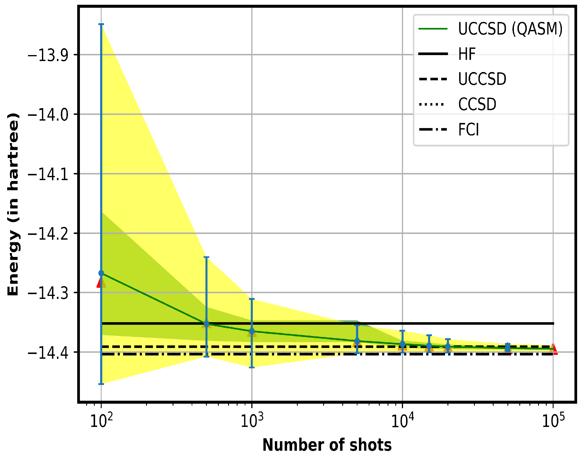
4.1. Analysis of the Required Number of Shots for QASM Calculations

We study the effect of the number of shots, for evaluating the ground state energy of the considered systems, on precision, for the results obtained using the QASM simulator. We chose the Be atom as a representative system in the STO-3G basis with Jordan–Wigner mapping for this purpose. The findings from a preliminary analysis of percentage fraction error with respect to FCI versus number of shots, with the latter verified up to 512 shots in steps of one, is given in Figure 4. We deemed this analysis as being qualitative, in that in a calculation with a given number of shots, the computation does not return identical results when repeated. Hence, we only pay attention to the overall trend for the purposes of this analysis. We note that each point on the X-axis in Figure 4 is an individual computation with those many shots. For 100 shots, we have approximately 4 percent error for Be, which is clearly not desirable. This leads us to Figure 2, which shows results from larger intervals, and all the way up to 100,000 shots. We also explicitly plot the energy versus the number of shots here. This analysis is rigorous, with the inclusion of maximum, minimum, and mean values for the energies at each data point, by repeating each of the runs for a given number of shots 160 times. In Figure 4, we also show the values of energy calculated on a classical computer from the HF, FCI, CCSD and UCCSD methods, so as to have a visual feel of correlation effects. It is noticeable from the above figure that at 100 shots, the mean energy is above the HF value, and therefore hardly satisfying the variational principle. One can also see that at lower number of shots, the error bar (the difference between the maximum and minimum values) is so large that its extent is greater than the difference between the energy values from the HF and FCI methods, that is, the amount of electron correlation. As the number of shots increase, the curve approaches and appears to converge to the UCCSD value that one obtains with a classical computer and has a very small error bar. It is worth noting here that had we increased the shots further, the curve would have, albeit gradually, yielded lower values. The inference that the curve would continue to monotonically decrease is based on a simple fit to the mean energy values. However, it is important to see that it is non-trivial to find a rigorous fit due to the statistical nature of each data points, and for our purposes, not necessary. The plot also shows that the error bars reduce with increasing shots. Based on these results, we performed computations with the QASM backend for the rest of the basis sets and mappings, as well as for the other atoms, setting the number of shots to 20,000. The rationale is that 20,000 shots finds a golden mean between computational cost and accuracy. In fact, we obtained about 0.1 percent error for the mean value with respect to FCI, while the standard deviation is only around 4 mHa. We also add at this point that we carried out bootstrapping procedure to check its agreement of the mean over 160 repetitions for a given number of shots. For the purpose of bootstrapping, we chose 50 samples of lists with each having four data points (we did repeat the procedure for longer lists (up to lists of length 50 and from 10 to 100,000 shots for each list length), and found that the results only change at ∼0.1 mHa from 10,000 shots onwards). We find that mean and bootstrapped mean agree at 1 mH at 20,000 shots. Lastly, in the interest of computational time, we only performed one calculation with 20,000 shots for each of the remaining cases (that is, Be with other mappings and also the remaining two atomic systems considered) and not with twenty repetitions, given that for Be with STO-3G basis and Jordan–Wigner mapping, at those many shots, the difference between the maximum and minimum values in twenty repetitions is less than 0.1 percent. We anticipated the error estimate to be similar for the rest of the cases, and under this assumption, we performed a single run for them. It is worth adding at this point that there are works in the literature that have made great strides in reducing the number of variational quantum eigensolver measurements for electronic structure [82,83,84,85]. Lastly, we note that this analysis serves an important purpose; our estimate for the number of shots required sets the tone for future analyses on atomic systems with the QASM backend, where we can strive to emulate a quantum computer more realistically, with the inclusion of noise models and error mitigation.

4.2. Analysis of Errors Due to Trotter Number

We verified the errors that may arise as result of setting the Trotter number in our simulation to one. For the Be atom in the STO-3G basis and with Jordan–Wigner mapping, we found that up to a Trotter step of 50, the error was at most ∼1 milli-hartree in ∼14 hartree. For Li with the same basis and mapping, the error was found to be as high as 0.2 milli-hartree in ∼7 hartree, and for B + , the error did not exceed 0.1 milli-hartree in ∼24 hartree. We also verify that we obtain similar estimates with parity and Bravyi–Kitaev mappings for all three chosen atomic systems. Hence, we set a conservative estimate that even with other basis sets and mappings, the error due to Trotter step would not exceed 0.01 percent. In other words, the error is negligible, and justifies setting Trotter number to one. We note that trottering U ( θ ) does not preserve particle number, and in that sense, one can view the comparison between variational quantum eigensolver results and FCI results as the deviation in our results from the expectation value of the correct particle number.

4.3. Main Results and Analysis

We examine the correlation effects in the ground state energies of the systems that we considered, in Table 1, Table 2, Table 3 and Table 4, with each table presenting results for a given basis set. Among these, Table 1 (and the accompanying Figure 3) gives the STO-3G results. We immediately see that for Be, the energies obtained using the statevector simulator agree to ∼ 0.1 milli-hartree, or about 0.001 percent error, with respect to FCI. We find similar differences for Li and B + for the STO-3G basis, whose results are also presented in Figure 3. In comparison, the correlation effects from FCI are about 50, 40, and 60 milli-hartree for Be, Li , and B + , respectively. Therefore, we can infer that quantum simulation with statevector simulator accounts for electron correlations very accurately in the STO-3G basis. This is perhaps not surprising, as a statevector simulator does not rely upon statistics built from repeated measurements in order to extract energy. We also present our results from a QASM simulator. They are all in good agreement with the unitary coupled-cluster results from a classical computer, and not with the FCI results as one may expect, due to our choice of the number of shots (20,000 of them) as seen earlier. In fact, the difference between the FCI and the unitary coupled-cluster QASM value (about 8 and 11 milli-hartree for parity and Bravyi–Kitaev mappings, respectively, and about 15 milli-hartree for Jordan–Wigner case), is comparable with that between the maximum and the minimum values (about 8 milli-hartree) for 20,000 shots from Figure 2.
A peculiar observation in the classical computing part of the results is that for all the considered basis sets, the CCSD result agrees better with the results from the FCI method than the UCCSD method. In principle, UCCSD is expected to capture more many-body effects than CCSD, with the caveat that the energy expression for the former does not naturally terminate, thereby relying upon the chosen truncation scheme to achieve the desired results. We suspect that the observed deviation is associated with the truncation scheme of the UCCSD method. To that end, we provide a fairly detailed explanation of the approach taken in the openfermion code to evaluating the UCCSD energy, and en route, explain the approximations and truncation involved in the procedure. The UCCSD energy is calculated using the familiar E = Φ 0 | e Θ H e Θ | Φ 0 . Rather than taking the conventional route of solving the UCCSD equations, obtain the amplitudes, and then solve the expression for energy while suitably terminating the series, the code aims at directly solving the expression for energy by matrix multiplications involving H and e Θ | Φ 0 . In order to do this, the second quantized creation and annihilation operators in the Hamiltonian and wave function are mapped to a string of tensor products of Pauli operators using the Jordan–Wigner transformation. The CCSD equations are solved in Pyscf or any other suitable program, and the t amplitudes (real) thus obtained are used in e Θ . The remaining step, and arguably the most important, is finding an efficient way of matrix multiplication. This boils down further to finding an efficient approach for multiplying an exponential matrix and a column vector. The algorithm from Al-Mohy and Higham [86] is adopted, where e t A B , where A is an n × n matrix, and B an n × n 0 matrix, with n 0 < < n , is evaluated by approximating the exponential as a [ m / m ] Pade approximant, which in turn is written as a truncated Taylor series. The backward error from such an algorithm would depend on the choice of an integer, s 1 , and m, which are in turn chosen by an appropriate recipe from their paper. On the other hand, the UCCSD energy obtained from qiskit simulators (where we have a compact circuit representation for exponentials, after Trotterization), E = Φ 0 | e Θ H e Θ | Φ 0 , have their own sources of errors, which we have studied in detail in our work. Given that the approaches are different, complex, and come with their own approximations, and also given that evaluating a matrix exponential is almost always non-trivial, a thorough study of the openfermion UCCSD algorithm over and above the details that we mentioned above is perhaps beyond the scope of this work. To that end, we have done the best that we can, which is to compare both the UCCSD results with the FCI result with the same single-particle basis.
Table 2 (and Figure 5) also shows the same results but obtained with the STO-6G basis. The results are an improvement over the earlier basis as evident by lowering of the calculated energies, although the qubit number is the same for a given system, since more functions are contracted in the STO-6G case. Not too surprisingly, the trends are very similar to those in the STO-3G basis.
We now proceed to examine the results obtained from bigger bases as shown in Table 3 and Table 4 (and the accompanying Figure 6 and Figure 7 respectively). We reiterate that QASM results are not computed for calculations using these two basis sets, in view of the requirement of a large number of shots to obtain a reasonably accurate result. We observe from the Table 3 that the effect of electron correlation on FCI energy is about 40, 30, and 50 in milli-hartree for Be, Li , and B + , respectively, whereas the difference in the correlation energies between FCI and quantum simulation are about 10 milli-hartree for all the systems. This discrepancy is possibly due to the slow convergence of the COBYLA optimizer. To check this, we choose the Jordan–Wigner mapping and the STO-3G basis set for a representative calculation, and increase the number of iterations to beyond the default maximum threshold of 1000 iterations (which we employ to report our results in this work). We found that while the percentage fraction error with respect to the FCI result is 10 3 at 1000 iterations, it decreases further to 10 4 at 2000 iterations. We expect that with the 3-21G basis as well as the 6-31G basis, the results would improve slightly with larger number of iterations, which comes with higher computational cost. Alternatively, one could employ an optimizer that converges faster, such as L-BFGS-B and conjugate gradient, which we find after a preliminary survey to have converged within a lesser number of iterations but not as smoothly as COBYLA.

4.4. Further Findings from Obtained Data

In the rest of the results section, we briefly present an assortment of important comments based on our findings.
Dependence of results on mapping scheme: It is known that the energy landscape close to the variational minimum is invariant with respect to the chosen encoding. It is, therefore, important to note that the observed difference in results across maps for the QASM simulator could be more a consequence of the error due to statistics associated with the backend, and not the actual difference, if any. En route to drawing this conclusion, we have explicitly verified that the errors due to trotterization and optimizer convergence have been checked and are found to be negligible, by choosing Be as a representative case and for all the three mapping schemes.
Preferred mapping scheme: We note that for a given atom, between different maps, the change in correlation energies even with the QASM backend is ∼1 milli-hartree, thus reinforcing that the correlation energy is not very sensitive to the mapping scheme. In this regard, the parity map is cheaper due to the reduction of two qubits, while giving results in agreement with other maps that are more qubit-expensive, and hence recommended for future atomic calculations of this nature.
STO-6G vs. 3-21G bases: The largest basis chosen in this work, namely the 6-31G basis, displays trends similar to the 3-21G counterpart. An observation about the results from the 3-21G basis is that the obtained FCI results (and hence, statevector results and predicted QASM results with 20,000 shots) are comparable to those from the STO-6G basis for Be (within 10 milli-hartree), whereas the 3-21G results are slightly better (about 60 milli-hartree) and much worse (about 100 milli-hartree) for the negative and positive ions, respectively, than the STO-6G basis. However, since the STO-6G basis uses 10 qubits while 3-21G demands 18 for the considered systems, the former is more attractive and should be preferred over the latter.
Trends in C 2 + : Since our goal in this pilot study is to assess precision with which one can capture correlation effects, and not really present an exhaustive survey of many systems, we have tried to select carefully a few systems and attempted to be rigorous in studying the influence of the knobs of the variational quantum eigensolver algorithm in deciding the precision in ground state energies. As an extension, we also comment on two other isoelectronic systems to Be. We explicitly verify that the trends, as one would expect, remain the same in C 2 + by calculating its energies within the STO-3G and STO-6G bases, for all three mappings, and compare with FCI, CCSD, and the UCCSD results from a classical algorithm, just as we did for the main systems considered in this work. Within each of the two bases, our statevector (SV) results differ at ∼ 0.1 mHa with respect to the FCI values, while for QASM backend (with 20,000 shots), they differ at ∼ 10s of mHa. We add that we have avoided the isoelectronic He 2 , as the STO series contracted basis sets have been designed in a way historically where there is no room for any correlation effects.
Variational quantum eigensolver results versus FCI in larger bases: Lastly, we attempt to address the question of the energy from a variational quantum eigensolver calculation being farther away from the FCI value in larger basis sets, as compared to the smaller ones. This could be due to the fact that with lesser qubits in a smaller basis and hence a limited number of virtuals, we miss a fewer excitations, whereas for a larger basis with more virtuals, we miss more excitations from the higher-level excitations such as from the triples and quadruples.

5. Conclusions

We investigated the trends in electron correlation effects for assessing the precision with which we can determine the ground state energies of Be, Li , and B + isoelectronic systems using the quantum-classical hybrid variational quantum eigensolver algorithm. We worked with four single-particle basis sets, two minimal and two split-valence, that are not very qubit-expensive and thus suited for the Noise Intermediate State Quantum era. Within each of those bases, we analyzed the changes in the results with choice of mapping as well as the backend simulator, in the unitary coupled-cluster theory ansätz. The energies obtained using the STO-3G basis showed that the statevector results agreed well beyond the milli-hartree level of precision with respect to the best possible calculation within that single-particle basis, namely the full configuration interaction method, for all the three atomic systems. Moreover, the results were found to be almost independent of the choice of mapping. For calculations using the QASM simulator backend, we first carried out an extensive analysis of the required number of shots, and with our recommended value, the results agreed to tens of milli-hartree with respect to the full configuration interaction method. We also probed the errors due to the spread in results from the repetition of a computation with a given number of shots, and found that they lie around the same ballpark, and the energies are in better agreement with the values obtained using the singles and doubles approximated unitary coupled-cluster theory on a classical computer. The results from the higher quality STO-6G basis also showed similar trends. When we examined the statevector results from the larger (in number of qubits) 3-21G basis set, we found that the values were comparable with those obtained using the STO-6G basis set and with the same backend, although the former required eight extra qubits than the latter. We find again that the results from the 3-21G basis agree better with the singles and doubles approximated unitary coupled-cluster theory. The results also vary within 10 milli-hartree across different mappings. The trends from the 6-31G basis are similar to those from the 3-21G basis set. Our work is timely and relevant in view of recent developments, such as the announcement of the IBM Quantum Condor, which is expected in 2023, which aims to hit the 1000-qubit mark in the quest for scaling quantum computers [87]. When such machines come to fruition, our pilot study will pave the way in extending our present calculations to not only heavier atomic systems, but also in evaluating other properties with the variational quantum eigensolver algorithm, which would be of interest in new physics beyond the Standard Model and other important applications such as atomic clocks.

Author Contributions

Conceptualization, B.K.S., S.P.V. and B.P.D.; Formal analysis, S. and S.P.V.; Investigation, S. and S.P.V.; Project administration, B.K.S. and B.P.D.; Software, S. and S.P.V.; Supervision, B.K.S. and B.P.D.; Validation, B.K.S., B.P.D., S.P.V. and S.; Writing—original draft, S. and S.P.V.; Writing—review and editing, B.K.S., B.P.D., S.P.V. and S. All authors have read and agreed to the published version of the manuscript.

Funding

This research received no external funding.

Institutional Review Board Statement

Not applicable.

Informed Consent Statement

Not applicable.

Data Availability Statement

The data that support the findings of this study are available from the corresponding author upon reasonable request.

Acknowledgments

We thank Ramanuj Mitra and Amar Vutha for their help with computational resources for the calculations reported in this work. We are also grateful to Kenji Sugisaki for useful discussions. Sumeet thanks Physical Research Laboratory (PRL), Ahmedabad and CQuERE, TCG CREST, Kolkata, for providing the visiting fellowship to carry out a part of this work. Most of the computations were performed on the VIKRAM-100 cluster at PRL and CDAC’s PARAM Siddhi machine. We acknowledge National Supercomputing Mission (NSM) for providing computing resources of ‘PARAM Siddhi-AI’ at C-DAC Pune, which is implemented by C-DAC and supported by the Ministry of Electronics and Information Technology (MeitY) and Department of Science and Technology (DST), Government of India. S.P.V. acknowledges the Graham cluster at the SciNet HPC Consortium (Compute Canada). SciNet is funded by: the Canada Foundation for Innovation; the Government of Ontario; Ontario Research Fund—Research Excellence; and the University of Toronto. S.P.V. and Sumeet both used Google Colab (Bisong E. (2019) Google Colaboratory. In: Building Machine Learning and Deep Learning Models on Google Cloud Platform. Apress, Berkeley, CA. https://doi.org/10.1007/978-1-4842-4470-8_7) for less compute intensive analyses.

Conflicts of Interest

The authors declare no conflict of interest or competing interests.

References

  1. Deutsch, I.H. Harnessing the Power of the Second Quantum Revolution. Phys. Rev. X Quantum 2020, 1, 020101. [Google Scholar] [CrossRef]
  2. McArdle, S.; Endo, S.; Aspuru-Guzik, A.; Benjamin, S.C.; Yuan, X. Quantum Computational Chemistry. Rev. Mod. Phys. 2020, 92, 015003. [Google Scholar] [CrossRef] [Green Version]
  3. Cade, C.; Mineh, L.; Montanaro, A.; Stanisic, S. Strategies for Solving the Fermi-Hubbard Model on Near-Term Quantum Computers. Phys. Rev. B 2020, 102, 235122. [Google Scholar] [CrossRef]
  4. Nam, Y.; Chen, J.S.; Pisenti, N.C.; Wright, K.; Delaney, C.; Maslov, D.; Kim, J. Ground-State Energy Estimation of the Water Molecule on a Trapped-Ion Quantum Computer. Nature J. Phys. Q. Info. 2020, 6, 33. [Google Scholar] [CrossRef]
  5. Takeshita, T.; Rubin, N.C.; Jiang, Z.; Lee, E.; Babbush, R.; McClean, J.R. Increasing the Representation Accuracy of Quantum Simulations of Chemistry without Extra Quantum Resources. Phys. Rev. X 2020, 10, 011004. [Google Scholar] [CrossRef] [Green Version]
  6. Low, G.H.; Chuang, I.L. Hamiltonian Simulation by Qubitization. Quantum 2019, 3, 163. [Google Scholar] [CrossRef] [Green Version]
  7. Sawaya, N.P.D.; Menke, T.; Kyaw, T.H.; Johri, S.; Aspuru-Guzik, A.; Guerreschi, G.G. Resource-Efficient Digital Quantum Simulation of d-Level Systems for Photonic, Vibrational, and Spin-s Hamiltonians. Nature J. Phys. Q. Info. 2020, 6, 49. [Google Scholar] [CrossRef]
  8. Chivilikhin, D.; Samarin, A.; Ulyantsev, V.; Iorsh, I.; Oganov, A.R.; Kyriienko, O. MoG-VQE: Multiobjective Genetic Variational Quantum Eigensolver. arXiv 2020, arXiv:2007.04424. [Google Scholar]
  9. Abrams, D.S.; Lloyd, S. Simulation of Many-Body Fermi Systems on a Universal Quantum Computer. Phys. Rev. Lett. 1997, 79, 2586. [Google Scholar] [CrossRef] [Green Version]
  10. Abrams, D.S.; Lloyd, S. Quantum Algorithm Providing Exponential Speed Increase for Finding Eigenvalues and Eigenvectors. Phys. Rev. Lett. 1999, 83, 5162. [Google Scholar] [CrossRef] [Green Version]
  11. Saue, T.; Bast, R.; Gomes, A.S.P.; Jensen, H.J.A.; Visscher, L.; Aucar, I.A.; van Stralen, J.N. The DIRAC Code for Relativistic Molecular Calculations. J. Chem. Phys. 2020, 152, 204104. [Google Scholar] [CrossRef] [PubMed]
  12. Aspuru-Guzik, A.; Dutoi, A.D.; Love, P.J.; Gordon, M.H. Simulated Quantum Computation of Molecular Energies. Science 2005, 309, 1704. [Google Scholar] [CrossRef] [PubMed] [Green Version]
  13. Lanyon, B.P.; Whitfield, J.D.; Gillett, G.G.; Goggin, M.E.; Almeida, M.P.; Kassal, I.; White, A.G. Towards Quantum Chemistry on a Quantum Computer. Nat. Chem. 2010, 2, 106. [Google Scholar] [CrossRef] [Green Version]
  14. Mohammadbagherpoor, H.; Oh, Y.H.; Dreher, P.; Singh, A.; Yu, X.; Rindos, A.J. An Improved Implementation Approach for Quantum Phase Estimation on Quantum Computers. arXiv 2019, arXiv:1910.11696. [Google Scholar]
  15. Paesani, S.; Gentile, A.A.; Santagati, R.; Wang, J.; Wiebe, N.; Tew, D.P.; O’Brien, J.L.; Thompson, M.G. Experimental Bayesian Quantum Phase Estimation on a Silicon Photonic Chip. Phys. Rev. Lett. 2017, 118, 100503. [Google Scholar] [CrossRef] [Green Version]
  16. Yung, M.H.; Casanova, J.; Mezzacapo, A.; McClean, J.R.; Lamata, L.; Aspuru-Guzik, A.; Solano, E. From Transistor to Trapped-Ion Computers for Quantum Chemistry. Sci. Rep. 2014, 4, 3589. [Google Scholar] [CrossRef] [Green Version]
  17. Peruzzo, A.; McClean, J.R.; Shadbolt, P.; Yung, M.H.; Zhou, X.Q.; Love, P.J.; Aspuru-Guzik, A.; O’Brien, J.L. A Variational Eigenvalue Solver on a Photonic Quantum Processor. Nat. Comm. 2014, 5, 4213. [Google Scholar] [CrossRef] [Green Version]
  18. Clarke, J.; Wilhelm, K.F. Superconducting Quantum Bits. Nature 2008, 453, 1031. [Google Scholar] [CrossRef]
  19. Cirac, J.I.; Zoller, P. Quantum Computations with Cold Trapped Ions. Phys. Rev. Lett. 1995, 74, 4091. [Google Scholar] [CrossRef]
  20. Kandala, A.; Mezzacapo, A.; Temme, K.; Takita, M.; Brink, M.; Chow, J.M.; Gambetta, J.M. Hardware-Efficient Variational Quantum Eigensolver for Small Molecules and Quantum Magnets. Nature 2017, 549, 242. [Google Scholar] [CrossRef]
  21. Wang, H.; Kais, S.; Aspuru-Guzik, A.; Hoffmann, M.R. Quantum Algorithm for Obtaining the Energy Spectrum of Molecular Systems. Phys. Chem. Chem. Phys. 2008, 10, 5388. [Google Scholar] [CrossRef] [PubMed] [Green Version]
  22. Colless, J.I.; Ramasesh, V.V.; Dahlen, D.; Blok, M.S.; Kimchi-Schwartz, M.E.; McClean, J.R.; Carter, J.; de Jong, W.A.; Siddiqi, I. Computation of Molecular Spectra on a Quantum Processor with an Error-Resilient Algorithm. Phys. Rev. X 2018, 8, 011021. [Google Scholar] [CrossRef] [Green Version]
  23. Wang, Y.; Dolde, F.; Biamonte, J.; Babbush, R.; Bergholm, V.; Yang, S.; Wrachtrup, J. Quantum Simulation of Helium Hydride Cation in a Solid-State Spin Register. Am. Chem. Soc. Nano 2015, 9, 7769. [Google Scholar] [CrossRef] [PubMed] [Green Version]
  24. Romero, J.; Babbush, R.; McClean, J.R.; Hempel, C.; Love, P.J.; Aspuru-Guzik, A. Strategies for Quantum Computing Molecular Energies using the Unitary Coupled Cluster Ansatz. Quantum Sci. Technol. 2019, 4, 014008. [Google Scholar] [CrossRef] [Green Version]
  25. Kumar, S.; Singh, R.P.; Behera, B.K.; Panigrahi, P.K. Quantum Simulation of Negative Hydrogen Ion using Variational Quantum Eigensolver on IBM Quantum Computer. arXiv 2019, arXiv:1903.03454v1. [Google Scholar]
  26. Schmidt-Kaler, F.; Pfau, T.; Schmelcher, P.; Schleich, W. Focus on Atom Optics and its Applications. New J. Phys. 2010, 12, 065014. [Google Scholar] [CrossRef]
  27. Chou, C.W.; Hume, D.B.; Rosenband, T.; Wineland, D.J. Optical Clocks and Relativity. Science 2010, 329, 1630. [Google Scholar] [CrossRef] [Green Version]
  28. Wansbeek, L.W.; Sahoo, B.K.; Timmermans, R.G.E.; Jungmann, K.; Das, B.P.; Mukherjee, D. Atomic Parity Nonconservation in Ra+. Phys. Rev. A 2008, 78, 050501. [Google Scholar] [CrossRef] [Green Version]
  29. Tiecke, T.G.; Thompson, J.D.; De Leon, N.P.; Liu, L.R.; Vuletic, V.; Lukin, M.D. Nanophotonic Quantum Phase Switch with a Single Atom. Nature 2014, 508, 241. [Google Scholar] [CrossRef] [Green Version]
  30. Fortson, N. Possibility of Measuring Parity Nonconservation With a Single Trapped Atomic Ion. Phys. Rev. Lett. 1993, 70, 2383. [Google Scholar] [CrossRef]
  31. Sahoo, B.K.; Das, B.P. Relativistic Normal Coupled-Cluster Theory for Accurate Determination of Electric Dipole Moments of Atoms: First Application to the 199Hg Atom. Phys. Rev. Lett. 2018, 120, 203001. [Google Scholar] [CrossRef] [PubMed] [Green Version]
  32. Sur, C.; Latha, K.V.P.; Sahoo, B.K.; Chaudhuri, R.K.; Das, B.P.; Mukherjee, D. Electric Quadrupole Moments of the D States of Alkaline-Earth-Metal Ions. Phys. Rev. Lett. 2006, 96, 193001. [Google Scholar] [CrossRef] [PubMed]
  33. Sahoo, B.K.; Das, B.P.; Spiesberger, H. New Physics Constraints from Atomic Parity Violation in 133Cs. Phys. Rev. D 2021, 103, L111303. [Google Scholar] [CrossRef]
  34. Kastberg, A.; Aoki, A.; Sahoo, B.K.; Sakemi, Y.; Das, B.P. Optical-Lattice-Based Method for Precise Measurements of Atomic Parity Violation. Phys. Rev. A 2019, 100, 050101. [Google Scholar] [CrossRef] [Green Version]
  35. Sakurai, A.; Sahoo, B.K.; Asahi, K.; Das, B.P. Relativistic Many Body Theory of the Electric Dipole Moment of 129Xe and its Implications for Probing New Physics Beyond the Standard Model. Phys. Rev. A 2019, 100, 020502. [Google Scholar] [CrossRef] [Green Version]
  36. Prasannaa, V.S.; Mitra, R.; Sahoo, B.K. Reappraisal of P, T-Odd Parameters from the Improved Calculation of Electric Dipole Moment of 225Ra Atom. J. Phys. B 2020, 53, 195004. [Google Scholar] [CrossRef]
  37. Guo, X.T.; Yu, Y.-M.; Liu, Y.; Suo, B.B.; Sahoo, B.K. Electric dipole and quadrupole properties of Cd atom for atomic clock applications. Phys. Rev. A 2021, 103, 013109. [Google Scholar] [CrossRef]
  38. Oskay, W.H.; Itano, W.M.; Bergquist, J.C. Measurement of the 199Hg+ 5d9 6s22D5/2 Electric Quadrupole Moment and a Constraint on the Quadrupole Shift. Phys. Rev. Lett. 2006, 94, 163001. [Google Scholar]
  39. Rosenband, T.; Schmidt, P.O.; Hume, D.B.; Itano, W.M.; Fortier, T.M.; Stalnaker, J.E.; Kim, K.; Diddams, S.A.; Koelemeij, J.C.J.; Bergquist, J.C.; et al. Observation of the 1S0 to 3P0 Clock Transition in 27Al+. Phys. Rev. Lett. 2007, 98, 220801. [Google Scholar] [CrossRef] [Green Version]
  40. Wilpers, G.; Oates, C.W.; Diddams, S.A.; Bartels, A.; Fortier, T.M.; Oskay, W.H.; Hollberg, L. Absolute frequency measurement of the neutral 40Ca optical frequency standard at 657 nm based on microkelvin atoms. Metrologia 2007, 44, 146. [Google Scholar] [CrossRef] [Green Version]
  41. Barber, Z.W.; Hoyt, C.; Oates, C.; Hollberg, L.; Taichenachev, A.; Yudin, V. Direct Excitation of the Forbidden Clock Transition in Neutral 174Yb Atoms Confined to an Optical Lattice. Phys. Rev. Lett. 2006, 96, 083002. [Google Scholar] [CrossRef] [PubMed] [Green Version]
  42. Ludlow, A.D.; Zelevinsky, T.; Campbell, G.K.; Blatt, S.; Boyd, M.M.; de Miranda, M.H.G.; Martin, M.J.; Thomsen, J.W.; Foreman, S.M.; Ye, J.; et al. Sr Lattice Clock at 1 × 10¹⁶ Fractional Uncertainty by Remote Optical Evaluation with a Ca Clock. Science 2008, 319, 1805. [Google Scholar] [CrossRef] [PubMed]
  43. Jefferts, S.R.; Shirley, J.; Parker, T.E.; Heavner, T.P.; Meekhof, D.M.; Nelson, C.; Walls, F.L. Accuracy evaluation of NIST-F1. Metrologia 2002, 39, 321. [Google Scholar] [CrossRef] [Green Version]
  44. Sahoo, B.K.; Ohayon, B. Benchmarking Many-body Approaches for the Determination of Isotope Shift Constants: Application to the Li, Be+ and Ar15+ Isoelectronic Systems. Phys. Rev. A 2021, 103, 052802. [Google Scholar] [CrossRef]
  45. Koszorús, Á; Yang, X.F.; Jiang, W.G.; Novario, S.J.; Bai, S.W.; Billowes, J.; Wilkins, S.G. Charge radii of exotic potassium isotopes challenge nuclear theory and the magic character of N=32. Nature Phys. 2021, 17, 439. [Google Scholar]
  46. Yu, Y.-M.; Sahoo, B.K.; Suo, B.B. Ground state gj factors of the Cd+, Yb+ and Hg+ ions. Phys. Rev. A 2020, 102, 062824. [Google Scholar] [CrossRef]
  47. Lindgren, I.; Morrison, J. Atomic Many-Body Theory; Springer: Berlin/Heidelberg, Germany, 1986. [Google Scholar]
  48. Kellö, V.; Urban, M.; Sadlej, A.J. Electric Dipole Polarizabilities of Negative Ions of the Coinage Metal Atoms. Chem. Phys. Lett. 1996, 253, 383. [Google Scholar] [CrossRef]
  49. Sahoo, B.K. Determination of the Dipole Polarizability of the Alkali-metal Negative Ions. Phys. Rev. A 2020, 102, 022820. [Google Scholar] [CrossRef]
  50. Andersen, T. Low-energy Outer-shell Photodetachment of the Negative Ion of Boron. Phys. Reps. 2004, 394, 157. [Google Scholar]
  51. Massey, H.S.W. Negative Ions, 3rd ed.; Cambridge University Press: London, UK; Cambridge University Press: New York, NY, USA, 1976. [Google Scholar]
  52. Dudinikov, V. Development and Applications of Negative Ion Sources; Springer Series on Atomic, Optical, and Plasma Physics, v. 110, Switzerland; Springer: Cham, Switzerland, 2019. [Google Scholar]
  53. Lim, I.S.; Schwerdtfeger, P. Four-component and Scalar Relativistic Douglas-Kroll Calculations for Static Dipole Polarizabilities of the Alkaline-earth-metal Elements and their Ions from Can to Ran (n=0,+1,+2). Phys. Rev. A 2004, 70, 062501. [Google Scholar] [CrossRef]
  54. Sahoo, B.K.; Das, B.P. Relativistic Coupled-cluster Studies of Dipole Polarizabilities in Closed-shell Atoms. Phys. Rev. A 2008, 77, 062516. [Google Scholar] [CrossRef] [Green Version]
  55. Singh, Y.; Sahoo, B.K.; Das, B.P. Correlation Trends in the Ground-state Static Electric Dipole Polarizabilities of Closed-shell Atoms and Ions. Phys. Rev. A 2013, 88, 062504. [Google Scholar] [CrossRef] [Green Version]
  56. Puchalski, M.; Komasa, J.; Pachucki, K. Testing Quantum Electrodynamics in the Lowest Singlet States of the Beryllium Atom. Phys. Rev. A 2013, 87, 030502. [Google Scholar] [CrossRef] [Green Version]
  57. Cook, E.C.; Vira, A.D.; Patterson, C.; Livernois, E.; Williams, W.D. Testing Quantum Electrodynamics in the Lowest Singlet State of Neutral Beryllium-9. Phys. Rev. Lett. 2018, 121, 053001. [Google Scholar] [CrossRef] [Green Version]
  58. Puchalski, M.; Pachucki, K.; Komasa, J. Isotope Shift in a Beryllium Atom, Phys. Rev. A 2014, 89, 012506. [Google Scholar] [CrossRef] [Green Version]
  59. McGeoch, M.W.; Sclier, R.E. Generation of Lithium Negative Ions in a Volume Source with Optical Pumping. J. Appl. Phys. 1987, 61, 4955. [Google Scholar] [CrossRef]
  60. Das, B.P.; Idrees, M. Some Theoretical Aspects of the Group-IIIA-ion Atomic Clocks: Intercombination Transition Probabilities. Phys. Rev. A 1990, 42, 6900. [Google Scholar] [CrossRef]
  61. Wineland, D.J.; (Department of Radiology and Nuclear Medicine, University Hospital Basel, Basel, Switzerland). Personal Communication, 2014.
  62. Gao, Q.; Nakamura, H.; Gujarati, T.P.; Jones, G.O.; Rice, J.E.; Wood, S.P.; Yamamoto, N. Computational Investigations of the Lithium Superoxide Dimer Rearrangement on Noisy Quantum Devices. arXiv 2019, arXiv:1906.10675. [Google Scholar] [CrossRef]
  63. Lolur, P.; Rahm, M.; Skogh, M.; Garcia-Alvarez, L.; Wendin, G. Benchmarking the Variational Quantum Eigensolver through Simulation of the Ground State Energy of Prebiotic Molecules on High-Performance Computers. arXiv 2021, arXiv:2010.1357. [Google Scholar]
  64. Zha, X.H.; Zhang, C.; Fan, D.; Xu, P.; Du, S.; Zhang, R.-Q.; Fu, C. The Impacts of Optimization Algorithm and Basis Size on the Accuracy and Efficiency of Variational Quantum Eigensolver. arXiv 2021, arXiv:2006.15852. [Google Scholar]
  65. Armaos, V.; Badounas, D.A.; Deligiannis, P.; Lianos, K. Computational Chemistry on Quantum Computers: Ground State Estimation. Appl. Phys. A 2020, 126, 625. [Google Scholar] [CrossRef]
  66. Tavares, C.; Oliveira, S.; Fernes, V.; Postnikov, A.; Vasilevskiy, M.I. Calculation of the Ground-state Stark Effect in Small Molecules Using the Variational Quantum Eigensolver. arXiv 2021, arXiv:2103.11743. [Google Scholar]
  67. Jones, N.C.; Whitfield, J.D.; McMahon, P.L.; Yung, M.H.; Meter, R.V.; Aspuru-Guzik, A.; Yamamoto, Y. Faster Quantum Chemistry Simulation on Fault-Tolerant Quantum Computers. N. J. Phys. 2012, 14, 115023. [Google Scholar]
  68. Seeley, J.T.; Richard, M.J.; Love, P.J. The Bravyi–Kitaev Transformation for Quantum Computation of Electronic Structure. J. Chem. Phys. 2012, 137, 224109. [Google Scholar] [CrossRef] [Green Version]
  69. Bravyi, S.; Gambetta, J.M.; Mezzacapo, A.; Temme, K. Tapering off Qubits to Simulate Fermionic Hamiltonians. arXiv 2017, arXiv:1701.08213. [Google Scholar]
  70. Bartlett, R.J.; Musial, M. Coupled-Cluster Theory in Quantum Chemistry. Revs. Mod. Phys. 2007, 79, 291. [Google Scholar] [CrossRef] [Green Version]
  71. Das, B.P.; Nayak, M.K.; Abe, M.; Prasannaa, V.S. Relativistic Many-Body Aspects of the Electron Electric Dipole Moment Searches Using Molecules. In Handbook of Relativistic Quantum Chemistry; Liu, W., Ed.; Springer: Berlin/Heidelberg, Germany, 2017. [Google Scholar]
  72. Kutzelnigg, W. Quantum chemistry in Fock space. I. The universal wave and energy operators. J. Chem. Phys. 1982, 77, 3081. [Google Scholar] [CrossRef]
  73. Sun, Q.; Berkelbach, T.C.; Blunt, N.S.; Booth, G.H.; Guo, S.; Li, Z.; Chan, G.K.L. PySCF: The Python-Based Simulations of Chemistry Framework, Wiley Interdisciplinary Reviews: Computational Molecular. Science 2017, 8, e1340. [Google Scholar]
  74. McClean, J.R.; Rubin, N.C.; Sung, K.J.; Kivlichan, I.D.; Bonet-Monroig, X.; Cao, Y.; Babbush, R. OpenFermion: The Electronic Structure Package for Quantum Computers. arXiv 2017, arXiv:1710.07629. [Google Scholar] [CrossRef]
  75. Boys, S.F. Electronic Wave Functions - I. A General Method of Calculation for the Stationary States of Any Molecular System. Proc. R. Soc. Lond. A 1950, 200, 542. [Google Scholar]
  76. Hehre, W.J.; Stewart, R.F.; Pople, J.A. Self-Consistent Molecular-Orbital Methods. I. Use of Gaussian Expansions of Slater-Type Atomic Orbitals. J. Chem. Phys. 1969, 51, 2657. [Google Scholar] [CrossRef]
  77. Ditchfield, R.; Hehre, W.J.; Pople, J.A. Self-Consistent Molecular-Orbital Methods. IX. An Extended Gaussian-Type Basis for Molecular-Orbital Studies of Organic Molecules. J. Chem. Phys. 1971, 54, 724. [Google Scholar] [CrossRef]
  78. Powell, M. Direct Search Algorithms for Optimization Calculations. Acta Numer. 1998, 7, 287. [Google Scholar] [CrossRef]
  79. Rattew, A.G.; Hu, S.; Pistoia, M.; Chen, R.; Wood, S. A Domain-agnostic, Noise-resistant, Hardware-efficient Evolutionary Variational Quantum Eigensolver. arXiv 2020, arXiv:1910.09694. [Google Scholar]
  80. Bös, J. Numerical Optimization of the Thickness Distribution of Three-Dimensional Structures With Respect to their Structural Acoustic Properties. Struct. Multidiscip. Optim. 2006, 32, 30. [Google Scholar] [CrossRef]
  81. Abraham, H. Qiskit: An Open-source Framework for Quantum Computing. 2019. Available online: https://zenodo.org/record/2562111#.YlamE-hBxPY (accessed on 1 December 2021). [CrossRef]
  82. Gokhale, P.; Angiuli, O.; Ding, Y.; Gui, K.; Tomesh, T.; Suchara., M.; Martonosi, M.; Chong, F.T. O(N3) Measurement Cost for Variational Quantum Eigensolver on Molecular Hamiltonians. IEEE Trans. Quantum Eng. IEEE Trans. Quantum Eng. 2020, 1, 1. [Google Scholar]
  83. Izmaylov, A.F.; Yen, T.C.; Ryabinkin, I.G. Revising the Measurement Process in the Variational Quantum Eigensolver: Is It Possible to Reduce the Number of Separately Measured Operators? Chem. Sci. 2019, 10, 3746. [Google Scholar] [CrossRef] [Green Version]
  84. Verteletskyi, V.; Yen, T.C.; Izmaylov, A.F. Measurement Optimization in the Variational Quantum Eigensolver using a Minimum Clique Cover. J. Chem. Phys. 2020, 152, 124114. [Google Scholar] [CrossRef]
  85. Zhao, A.; Tranter, A.; Kirby, W.M.; Ung, S.F.; Miyake, A.; Love, P.J. Measurement Reduction in Variational Quantum Algorithms. Phys. Rev. A 2020, 101, 062322. [Google Scholar] [CrossRef]
  86. Al-Mohy, A.H.; Higham, N.J. Computing the Action of the Matrix Exponential, with an Application to Exponential Integrators. SIAM J. Sci. Comput. 2011, 33, 488. [Google Scholar] [CrossRef]
  87. Gambetta, J.M. IBM’s Roadmap for Scaling Quantum Technology. Available online: https://www.ibm.com/blogs/research/2020/09/ibm-quantum-roadmap/ (accessed on 1 December 2021).
Figure 1. (a) A schematic demonstrating evaluation procedure of Equation (1) using the variational quantum eigensolver algorithm. It includes different combinations of mapping (in green), basis sets (in blue), and backend simulator (in red) to capture the correlation effects. A sample template unitary coupled-cluster circuit is provided for the case of three qubits ( q 0 , q 1 , and q 2 ), built out of CNOT and R z ( 2 θ ) gates. The figure lists the atomic systems chosen for the investigation, and it also mentions about the comparison of our variational quantum eigensolver results with those obtained on a classical computer by employing various many-body methods. (b) An overview of the variational quantum eigensolver algorithm applied to electronic structure problem, which requires generating the one-body and two-body integrals of atomic Hamiltonian, expressing the wave function in parametric form and adopting quantum modules for computation. The guess parameters are then updated each time in an iterative procedure on a classical optimizer until a global minimum is reached.
Quantumrep 04 00012 g001
Figure 2. Analysis of the unitary coupled cluster energy from the QASM backend (UCCSD(QASM)) versus the number of shots, for Be in STO-3G basis and with Jordan–Wigner mapping. The results obtained using the QASM backend are also compared with the values obtained using the full configuration interaction (FCI), coupled cluster in singles and doubles approximation (CCSD), and the unitary coupled cluster in the singles and doubles approximation (UCCSD) methods on a classical computer. Each data point (circle) represents the mean of 160 runs for a given number of shots, and is accompanied by two error bars, with the band in yellow quoting the range (maximum–minimum), while the green band denotes the standard deviation. The data points marked with a triangle refer to the bootstrapped mean. The CCSD and the FCI lines overlap exactly, owing to their agreement to the fifth decimal place, as Table 1 shows.
Quantumrep 04 00012 g002
Figure 3. Graphical illustration of results for the (a) Be, (b) Li , and (c) B + in STO-3G basis obtained using the variational quantum eigensolver algorithm. The figure serves to compare the impact of different combinations of fermion to qubit mapping techniques, namely Jordan–Wigner (JW), parity (PAR), and Bravyi–Kitaev (BK) transformations, as well as backend simulators (statevector and QASM). The dark blue bars indicate the energies obtained on a QASM simulator, while the bars in light blue specify the energies computed using a statevector simulator. The calculated energies are compared with full configuration interaction (FCI) (dot-dash line), and also with CCSD (dotted line), and UCCSD (dashed line) methods. Each of the plots also show the Hartree-Fock (HF) energy as a black solid line, which allows to visualize the correlation effects.
Quantumrep 04 00012 g003
Figure 4. Plot showing the variation in the percentage fraction error in the calculated energy using the QASM simulator with respect to the Full Configuration Interaction value, with the number of shots up to 512, for Be in the STO-3G basis and with the Jordan–Wigner mapping.
Quantumrep 04 00012 g004
Figure 5. Figure showing bar plots depicting the values of ground state energies of the (a) Be, (b) Li , and (c) B + obtained from variational quantum eigensolver calculations in the STO-6G basis, with various fermion to qubit mapping techniques, and on different backend simulators. The notations are the same as in Figure 3.
Quantumrep 04 00012 g005
Figure 6. Our results for the ground state energies of the (a) Be, (b) Li , and (c) B + in 3-21G basis using different combinations of mappings and backend simulators visualized as bar plots. The notations that have been adopted for this figure are the same as those for Figure 3.
Quantumrep 04 00012 g006
Figure 7. The results for the energies of the (a) Be, (b) Li , and (c) B + in the 6-31G basis in the form of bar plots showing different combinations of fermion to qubit mapping techniques and backend simulators. The notations that have been adopted for this figure are the same as those for Figure 3.
Quantumrep 04 00012 g007
Table 1. A quantitative analysis of the ground state energies (in hartree) of Be, Li , and B + computed using the variational quantum eigensolver algorithm in the STO-3G basis and adopting the UCCSD ansätz, with different combinations of simulators (statevector (SV) and QASM) and fermion to qubit mapping techniques (JW refers to Jordan–Wigner, PAR to parity, and BK to the Bravyi–Kitaev mapping). The results are compared with values obtained using various methods in a classical computer (ClC). Next to the final values, we provide the correlation energy for that combination in brackets. The percentage fraction difference with respect to FCI results is denoted as ‘ Δ in %’.
MapMethodBackendBeLi B +
HF −14.351880−7.213273−23.948470
ClCFCI −14.403655 (−0.051775)−7.253791 (−0.040518)−24.009814 (−0.061344)
CCSD −14.403651 (−0.051771)−7.253786 (−0.040513)−24.009811 (−0.061341)
UCCSD −14.391028 (−0.039148)−7.244008 (−0.030735)−23.994757 (−0.046287)
UCCSDQASM−14.388109 (−0.036229)−7.244270 (−0.030997)−24.002041 (−0.053571)
JW( Δ in %) ( 0.108 )( 0.131 )( 0.032 )
UCCSDSV−14.403490 (−0.05161)−7.253682 (−0.040409)−24.009652 (−0.061182)
( Δ in %) ( 0.001 )( 0.001 )( 0.001 )
UCCSDQASM−14.394762 (−0.042882)−7.243156 (−0.029883)−23.992675 (−0.044205)
PAR( Δ in %) ( 0.062 )( 0.146 )( 0.071 )
UCCSDSV−14.403446 (−0.051566)−7.253611 (−0.040338)−24.009631 (−0.061161)
( Δ in %) ( 0.001 )( 0.002 )( 0.001 )
UCCSDQASM−14.392365 (−0.040485)−7.243775 (−0.030502)−23.998311 (−0.049841)
BK( Δ in %) ( 0.078 )( 0.138 )( 0.048 )
UCCSDSV−14.403539 (−0.051659)−7.253681 (−0.040408)−24.009500 (−0.06103)
( Δ in %) ( 0.001 )( 0.001 )( 0.001 )
Table 2. The ground state energies of Be, Li , and B + obtained using the STO-6G basis. All notations are the same as in Table 1.
MapMethodBackendBeLi B +
HF −14.503361−7.295246−24.190562
ClCFCI −14.556088 (−0.052727)−7.336640 (−0.041394)−24.252889 (−0.062327)
CCSD −14.556083 (−0.052722)−7.336635 (−0.041389)−24.252884 (−0.062322)
UCCSD −14.543257 (−0.039896)−7.326677 (−0.031431)−24.237615 (−0.047053)
UCCSDQASM−14.544091 (−0.04073)−7.326529 (−0.031283)−24.227757 (−0.037195)
JW( Δ in %) ( 0.082 )( 0.138 )( 0.055 )
UCCSDSV−14.555940 (−0.052579)−7.336485 (−0.041239)−24.252614 (−0.062052)
( Δ in %) ( 0.001 )( 0.002 )( 0.001 )
UCCSDQASM−14.541160 (−0.037799)−7.321997 (−0.026751)−24.222150 (−0.031588)
PAR( Δ in %) ( 0.103 )( 0.199 )( 0.127 )
UCCSDSV−14.555943 (−0.052582)−7.336510 (−0.041264)−24.252623 (−0.062061)
( Δ in %) ( 0.001 )( 0.002 )( 0.001 )
UCCSDQASM−14.548048 (−0.044687)−7.321989 (−0.026743)−24.241578 (−0.051016)
BK( Δ in %) ( 0.055 )( 0.199 )( 0.047 )
UCCSDSV−14.555848(−0.052487)−7.336462 (−0.041216)−24.252669 (−0.062107)
( Δ in %) ( 0.002 )( 0.002 )( 0.001 )
Table 3. The table presents the energies for Be, Li , and B + in the 3-21G basis. The same notations as in Table 1 are adopted here.
MapMethodBackendBeLi B +
HF −14.486820−7.366760−24.096376
ClCFCI −14.531444 (−0.044624)−7.397779 (−0.031019)−24.153344 (−0.056968)
CCSD −14.531416 (−0.044596)−7.397757 (−0.030997)−24.153311 (−0.056935)
UCCSD −14.512130 (−0.02531)−7.383818 (−0.017058)−24.131129 (−0.034753)
JWUCCSDSV−14.513922 (−0.027102)−7.385692 (−0.018932)−24.138757 (−0.042381)
( Δ in %) ( 0.121 )( 0.163 )( 0.059 )
PARUCCSDSV−14.516600 (−0.02978)−7.387247 (−0.020487)−24.139378 (−0.043002)
( Δ in %) ( 0.102 )( 0.142 )( 0.058 )
BKUCCSDSV−14.519369 (−0.032549)−7.386396 (−0.019636)−24.139013 (−0.042637)
( Δ in %) ( 0.083 )( 0.154 )( 0.059 )
Table 4. Using the same notations as in Table 1, the ground state and correlation energies for Be, Li , and B + in the 6-31G basis are given.
MapMethodBackendBeLi B +
HF −14.566764−7.405387−24.234041
ClCFCI −14.613545 (−0.046781)−7.438753 (−0.033366)−24.293125 (−0.059084)
CCSD −14.613518 (−0.046754)−7.438739 (−0.033352)−24.293096 (−0.059055)
UCCSD −14.593071 (−0.026307)−7.423171 (−0.017784)−24.269635 (−0.035594)
JWUCCSDSV−14.601323 (−0.034559)−7.426886 (−0.021499)−24.279715 (−0.045674)
( Δ in %) ( 0.083 )( 0.159 )( 0.055 )
PARUCCSDSV−14.597296 (-0.111)−7.425017 (-0.185)−24.278157 (-0.061)
( Δ in %) (−0.030532)(−0.01963)(−0.044116)
BKUCCSDSV−14.597296 (−0.030532)−7.423154 (−0.017767)−24.277312 (−0.043271)
( Δ in %) ( 0.111 )( 0.209 )( 0.651 )
Publisher’s Note: MDPI stays neutral with regard to jurisdictional claims in published maps and institutional affiliations.

