Bose–Einstein Condensation Processes with Nontrivial Geometric Multiplicities Realized via 𝒫𝒯−Symmetric and Exactly Solvable Linear-Bose–Hubbard Building Blocks

Abstract

It is well known that, using the conventional non-Hermitian but $\mathcal{PT}-$symmetric Bose–Hubbard Hamiltonian with real spectrum, one can realize the Bose–Einstein condensation (BEC) process in an exceptional-point limit of order N. Such an exactly solvable simulation of the BEC-type phase transition is, unfortunately, incomplete because the standard version of the model only offers an extreme form of the limit, characterized by a minimal geometric multiplicity $K = 1$. In our paper, we describe a rescaled and partitioned direct-sum modification of the linear version of the Bose–Hubbard model, which remains exactly solvable while admitting any value of $K\ge 1$. It offers a complete menu of benchmark models numbered by a specific combinatorial scheme. In this manner, an exhaustive classification of the general BEC patterns with any geometric multiplicity is obtained and realized in terms of an exactly solvable generalized Bose–Hubbard model.

1. Introduction

The conceptual appeal of $\mathcal{PT}-$symmetry (i.e., of the parity times time reversal symmetry) currently influences several different areas of theoretical and/or experimental physics [1,2] as well as of the related mathematical physics [3,4,5]. The birth of the concept dates back to the mathematics of perturbation theory [6,7,8,9,10], but the real start of popularity was only inspired by Bender and Boettcher’s 1998 conjecture [11] that $\mathcal{PT}-$symmetry of a Hamiltonian H could play a key role in a “non-Hermitian” formulation of quantum mechanics of bound states (cf. reviews [12,13,14]).

One of the basic innovations connected with the use of non-Hermitian but $\mathcal{PT}-$symmetric Hamiltonians with real bound-state spectra has been found to lie in a remarkable and highly exciting possibility of a direct and experimentally controllable access to the dynamical regime of a spontaneous breakdown of the symmetry. Bender with Boettcher [11] were probably the first who managed to simulate this process (leading to a quantum phase transition, i.e., to an abrupt loss of the observability of the energy), using various elementary one-dimensional single-particle local potentials. This proved inspiring and influenced the model building efforts in multiple areas of realistic phenomenological considerations. Among others, several research teams turned also attention to a family of multiparticle $\mathcal{PT}-$symmetric benchmark Hamiltonians H called Bose–Hubbard models (see, for example, [15,16]).

The source of the appeal of the latter models lied in the possibility of a sufficiently realistic simulation of a specific quantum phase transition called Bose–Einstein condensation (BEC). From our present point of view, the most inspiring analysis was performed in [17], where a thorough mathematical description of the BEC phenomenon was performed, using both the linear (i.e., solvable, mathematically less complicated) and non-linear (i.e., fully general while just perturbative or purely numerical) versions of the underlying standard $\mathcal{PT}-$symmetric Bose–Hubbard Hamiltonian.

In both of these model-building arrangements, the process of the condensation is attributed, in Kato’s language [18], to the presence of higher-order exceptional points. In our present paper, we intend to study the former mechanism of the quantum phase transition in more detail, extending the scope of the approach to certain more general dynamical scenarios characterized by nontrivial, optional geometric multiplicities of the generic exceptional-point degeneracies.

2. Bose-Einstein Condensation

2.1. $\mathcal{PT}-$Symmetric Bose–Hubbard Model

For introduction, let us follow the guidance provided by Graefe et al. [17], who performed a detailed perturbation–approximation analysis of the $\mathcal{PT}-$symmetric Bose–Hubbard (BH) system living in a small vicinity of its BEC dynamical singularity. One of the most elementary versions of their non-Hermitian and BEC-supporting family of Hamiltonians had the following one-parametric form written in terms of the conventional creation and annihilation operators:

$${\widehat{H}}_{}\left(\gamma \right) = \left(a_1^{†}{a}_2+a_2^{†}{a}_1\right)-\mathrm{i}\gamma \left(a_1^{†}{a}_1-a_2^{†}{a}_2\right),\gamma \in (0,1).$$

(1)

As long as such a Hamiltonian commutes with the operator of the number of bosons as follows:

$$\widehat{\mathcal{N}} = a_1^{†}{a}_1+a_2^{†}{a}_2$$

(2)

(with eigenvalues $N_B = 1,2,\dots$), the model becomes exactly solvable, with the following spectrum:

$$E_n^{}\left(\gamma \right) = n\sqrt{1-{\gamma }^2},n\in \mathcal{S}\left(N\right),N = N_B+1$$

(3)

where

$$\mathcal{S}\left(N\right) = \{1-N,3-N,\dots ,N-3,N-1\}.$$

(4)

At $\gamma \in (0,1)$, the most characteristic features of such a spectrum are its reality, equidistance and up–down symmetry; see, for illustration, Figure 1 where we choose $N = 8$. In the picture, we see how the spectrum shrinks from the $\gamma = 0$ maximum {$-7,-5,-3,-1,1,3,5,7$} to a complete degeneracy at ${\gamma }^{} = {\gamma }^{\left(BEC\right)} = 1$. A detailed derivation of formula (3) itself can be found in [17].

In the framework of our present project, it is important that the operator version (1) of the unperturbed BH Hamiltonian may be studied, most efficiently, in its explicit infinite-dimensional block-diagonal matrix form as derived in [17]:

$$H_{}\left(\gamma \right) = \left(\begin{array}{cccc}{H}_{}^{\left(2\right)}\left(\gamma \right)& 0& 0& \dots \\ 0& H_{}^{\left(3\right)}\left(\gamma \right)& 0& \\ 0& 0& H_{}^{\left(4\right)}\left(\gamma \right)& \ddots \\ ⋮& & \ddots & \ddots \end{array}\right).$$

(5)

Each block $H_{}^{\left(N\right)}\left(\gamma \right)$ is a tridiagonal N by N matrix such that the following holds:

$$H_{}^{\left(2\right)}\left(\gamma \right) = \left[\begin{array}{cc}-i\gamma & 1\\ 1& i\gamma \end{array}\right],H_{}^{\left(3\right)}\left(\gamma \right) = \left[\begin{array}{ccc}-2i\gamma & \sqrt{2}& 0\\ \sqrt{2}& 0& \sqrt{2}\\ 0& \sqrt{2}& 2i\gamma \end{array}\right],$$

(6)

$$H_{}^{\left(4\right)}\left(\gamma \right) = \left[\begin{array}{cccc}-3\mathrm{i}\gamma & \sqrt{3}& 0& 0\\ \sqrt{3}& -\mathrm{i}\gamma & 2& 0\\ 0& 2& \mathrm{i}\gamma & \sqrt{3}\\ 0& 0& \sqrt{3}& 3\mathrm{i}\gamma \end{array}\right],H_{}^{\left(5\right)}\left(\gamma \right) = \left[\begin{array}{ccccc}-4\mathrm{i}\gamma & 2& 0& 0& 0\\ 2& -2\mathrm{i}\gamma & \sqrt{6}& 0& 0\\ 0& \sqrt{6}& 0& \sqrt{6}& 0\\ 0& 0& \sqrt{6}& 2\mathrm{i}\gamma & 2\\ 0& 0& 0& 2& 4\mathrm{i}\gamma \end{array}\right],$$

etc. This representation of the Hamiltonian reconfirms the conservation of the number of bosons $N_B = N-1$. At every N, the bound-state Schrödinger equation degenerates to a linear algebraic eigenvalue problem, yielding the closed-form eigenvalues (3). In this representation of the system, also the construction of the wave functions becomes tractable non-numerically [19].

2.2. BEC-Formation Patterns

The properties of spectrum (3) are reflected by the equidistance of the $N-$dependent set (4) of the energy-level quantum numbers. The degeneracy of all of the levels in the BEC limit $\gamma \to 1$ is simultaneous as follows:

$$\underset{\gamma \to 1}{lim}{E}_n^{}\left(\gamma \right) = {\eta }^{\left(N\right)} = 0,n\in \mathcal{S}\left(N\right).$$

(7)

An analogous degeneracy also controls the behavior of all of the eigenstates $|{\psi }_n^{}(N,\gamma )\rangle$ of the BH operator (1):

$$\underset{\gamma \to 1}{lim}|{\psi }_n^{}(N,\gamma )\rangle = |{\chi }_{\left(BEC\right)}^{\left(N\right)}\rangle ,n\in S\left(N\right),N = 2,3,\dots .$$

(8)

Precisely, such a degeneracy can be interpreted as one of the explicit realizations of the so-called Kato’s exceptional point of order N (EPN, [18]).

The physical limit $\gamma \to {\gamma }^{\left(BEC\right)} = 1$ and the mathematical limit $\gamma \to {\gamma }^{\left(EPN\right)} = 1$ appear synonymous. Unfortunately, such a correspondence between mathematics and physics is one-sided. In the context of mathematics, the convergence (8) towards a single limiting vector $|{\chi }_{\left(BEC\right)}^{\left(N\right)}\rangle$ must be considered a simplification and an artifact of the model. In any sufficiently model-independent scenario, it will be necessary to replace property (8) (where the EPN merger has the so called geometric multiplicity K equal to one) by the more general, $K-$centered eigenvector-degeneracy pattern with any geometric multiplicity $K\ge 1$ as follows:

$$\underset{\gamma \to {\gamma }^{\left(EPN\right)}}{lim}|{\psi }_{n_k}^{\left(EPN\right)}\left(\gamma \right)\rangle = |{\chi }_k^{\left(EPN\right)}\rangle ,n_k\in S_k^{\left(EPN\right)},k = 1,2,\dots ,K,$$

(9)

$$S_1^{\left(EPN\right)}\oplus S_2^{\left(EPN\right)}\oplus \dots \oplus S_K^{\left(EPN\right)} = \mathcal{S}\left(N\right).$$

(10)

The complete set $\mathcal{S}\left(N\right)$ of the energy quantum numbers must be admitted to be, in general, decomposed into a $K-$plet of disjoint subsets. Now, the main question to be addressed in our present paper is whether the generalized mathematical form (9) of the EPN limit with arbitrary $K\ge 1$ could still be assigned a suitable physical multi-bosonic interpretation via an exactly solvable BEC-supporting Hamiltonian, say, of the BH type.

3. Nontrivial Geometric Multiplicities $\mathbf{K}$ at Small $\mathbf{N}$

In our recent heuristic study [20] we addressed the problem on a purely methodical level. In a trial-and-error search for the low-dimensional toy-model matrix Hamiltonian with nontrivial geometric multiplicity of its degenerate EPN limit, we used the brute-force numerical methods and performed the search among certain real and more or less randomly selected matrices $H^{\left(6\right)}$. The inspection of the parametric-dependence of the spectra led us to the empirical conclusion and conjecture of a one-to-one correspondence between the trivial geometric multiplicity $K = 1$ of the exceptional points and the tridiagonality of the matrix $H^{\left(6\right)}$ in question.

This turned our attention to non-tridiagonal toy models $H^{\left(6\right)}$. The hypothesis appeared to work. Several models supporting the existence of exceptional points with $K = 2$ and $K = 3$ were identified. Unfortunately, our subsequent tentative extension of the brute-force empirical search to higher N encountered severe technical obstacles. Our conclusions formulated in [20] were, therefore, discouraging and skeptical. We argued that beyond $N\approx 6$, the numerical EPN searches become ill-conditioned, yielding highly unstable results marred, in the methodical context, by the influence of the ubiquitous rounding errors (for details see, in particular, Appendix A in [20]).

In our present paper, we decided to accept a different strategy. It will be based on a non-numerical, strictly analytic specification of the candidates for the suitable EPN-supporting toy-model Hamiltonians. For this purpose, we will merely rescale the separate fixed$-N$ components of the $K = 1$ Hamiltonian (5), yielding the trivially modified tilded forms of its submatrices, viz., the following:

$$c_k{H}_{}^{\left(2\right)}\left(\gamma \right) = \left[\begin{array}{cc}-i\gamma c_k& c_k\\ c_k& i\gamma c_k\end{array}\right] = \widetilde{H_{\left(c_k\right)}^{\left(2\right)}}\left(\gamma \right),c_k{H}_{}^{\left(3\right)}\left(\gamma \right) = \left[\begin{array}{ccc}-2i\gamma c_k& \sqrt{2}{c}_k& 0\\ \sqrt{2}{c}_k& 0& \sqrt{2}{c}_k\\ 0& \sqrt{2}{c}_k& 2i\gamma c_k\end{array}\right] = \widetilde{H_{\left(c_k\right)}^{\left(3\right)}}\left(\gamma \right)$$

(11)

etc. Obviously, any such a rescaling with real $c_k = c_k^{\left(N\right)}\ne 0$ preserves not only the basic features of physics behind the model but also, at any dimension $N = N_B+1$, the exact solvability of Schrödinger equation. At the same time, the new, alternative, non-tridiagonal candidates for the submatrices of the generalized $K>1$ versions of Hamiltonian (5) can tentatively be constructed using suitable direct-sum combinations of the building-blocks (11).

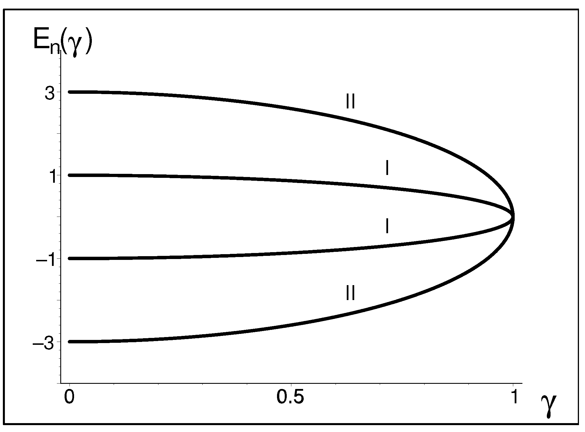
3.1. Three Bosons and $K = 2$

The first two simplest BH models with $N_B = N-1 = 1$ and $N_B = N-1 = 2$ are trivial, offering just the usual unique option with $K = 1$. Thus, our search for alternatives has to start from the next, $N = 4$ item taken from the $K = 1$ sequence of Hamiltonians (6), with the spectrum displayed in Figure 2. In the picture, we marked the levels by symbols “I” and “II” in order to indicate that precisely the same $\gamma -$dependent spectrum can be also generated by an alternative Hamiltonian defined as a direct sum of the two $N = 2$ matrices taken out of the tilded menu (11). This yields the innovated, $K = 2$ Hamiltonian as follows:

$$\widetilde{H_{\left(1\right)}^{\left(2\right)}}\left(\gamma \right)\oplus \widetilde{H_{\left(3\right)}^{\left(2\right)}}\left(\gamma \right) = \left[\begin{array}{cccc}-\mathrm{i}\gamma & 1& 0& 0\\ 1& \mathrm{i}\gamma & 0& 0\\ 0& 0& -3\mathrm{i}\gamma & 3\\ 0& 0& 3& 3\mathrm{i}\gamma \end{array}\right]\sim \left[\begin{array}{cccc}-3\mathrm{i}\gamma & 0& 0& 3\\ 0& -\mathrm{i}\gamma & 1& 0\\ 0& 1& \mathrm{i}\gamma & 0\\ 3& 0& 0& 3\mathrm{i}\gamma \end{array}\right] = H_{[K=2]}^{\left(4\right)}\left(\gamma \right)$$

(12)

characterized by the choice of scalings $c_1=1$ (levels “I”) and $c_2 = 3$ (levels “II”).

Besides sharing the spectrum (but not the eigenvectors!) with its BH predecessor $H_{[K = 1]}^{\left(4\right)}\left(\gamma \right)$ of Equation (6), the new model also illustrates several other merits of the present philosophy. The key point is that the two alternative isospectral Hamiltonians can be both made $\mathcal{PT}-$symmetric, and that their imaginary parts can be kept the same (i.e., diagonal). In this sense, we can treat the right-hand-side matrix in (12) as a canonical non-tridiagonal form of the $K = 2$ alternative to the original $K = 1$ BH building block at $N = 4$.

The existence of the two isospectral models with different eigenvectors may be interpreted as forcing us to introduce a new, ad hoc quantum number (e.g., “color”). Certainly, any less formal specification of such a quantum number (or numbers) would have to be left to the experimentalists. Near the BEC dynamical regime, only a dedicated experiment performed over the $N_B-$plet of bosons will be able to distinguish between the systems with different structures of wave functions. With their energy spectra fitted by the $K-$independent Formula (3), the measurements would also have to extract information about some wave function–dependent mean values of some other suitable observables.

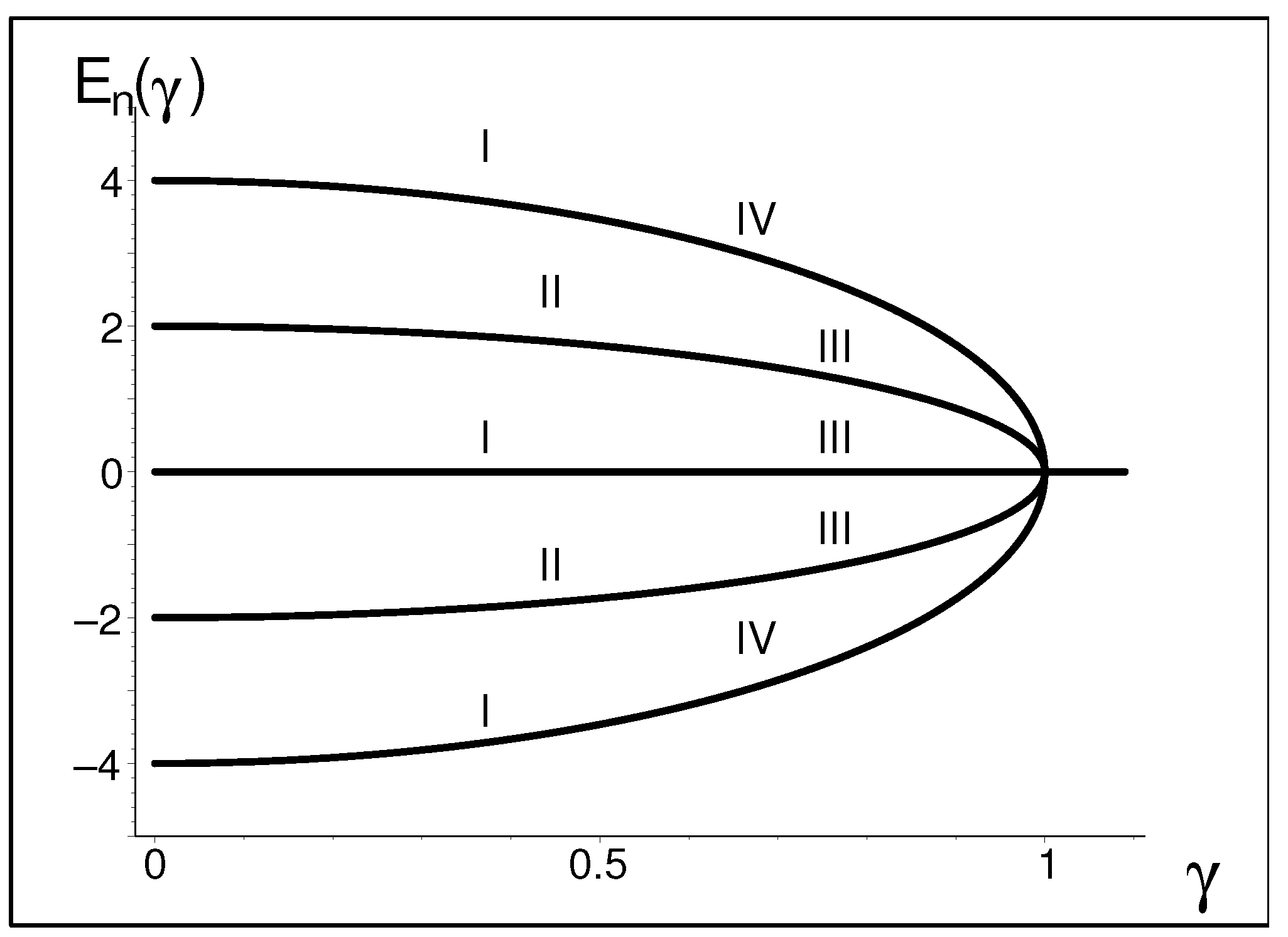
3.2. Four Bosons and $K = 2$

At $N = 5$ the $K = 1$ Hamiltonian $H^{\left(5\right)}\left(\gamma \right)$ of sequence (6) yields the “colorless” five-level spectrum as displayed in Figure 3. The elementary combinatorics reveals that besides such an option, we can now introduce the two alternative labelings “I + II” and “III + IV” of the states with $K = 2$. Having opted for “I + II” (see the picture) we are able to reproduce the spectrum by the direct product as follows:

$$\widetilde{H_{\left(2\right)}^{\left(3\right)}}\left(\gamma \right)\oplus \widetilde{H_{\left(2\right)}^{\left(2\right)}}\left(\gamma \right)\sim \left[\begin{array}{ccccc}-4\mathrm{i}\gamma & 0& 2\sqrt{2}& 0& 0\\ 0& -2\mathrm{i}\gamma & 0& 2& 0\\ 2\sqrt{2}& 0& 0& 0& 2\sqrt{2}\\ 0& 2& 0& 2\mathrm{i}\gamma & 0\\ 0& 0& 2\sqrt{2}& 0& 4\mathrm{i}\gamma \end{array}\right] = H_{[K=2]}^{\left(5\right)}(\gamma ,I+II)$$

(13)

(where $c_1 = c_2 = 2$) while in the second scenario, we choose $c_1 = 1$ and $c_2 = 4$ and have the following:

$$\widetilde{H_{\left(1\right)}^{\left(3\right)}}\left(\gamma \right)\oplus \widetilde{H_{\left(4\right)}^{\left(2\right)}}\left(\gamma \right)\sim \left[\begin{array}{ccccc}-4\mathrm{i}\gamma & 0& 0& 0& 4\\ 0& -2\mathrm{i}\gamma & \sqrt{2}& 0& 0\\ 0& \sqrt{2}& 0& \sqrt{2}& 0\\ 0& 0& \sqrt{2}& 2\mathrm{i}\gamma & 0\\ 4& 0& 0& 0& 4\mathrm{i}\gamma \end{array}\right] = H_{[K=2]}^{\left(5\right)}(\gamma ,III+IV).$$

(14)

We again decided to arrange the basis in such a manner that the main diagonals remain unchanged. This renders the resulting Hamiltonian submatrices sparse, multidiagonal, complex symmetric [21] and manifestly $\mathcal{PT}-$symmetric.

4. BEC Models of Any Dimension $\mathbf{N}$ and Multiplicity $\mathbf{K}$

4.1. Canonical Representation

In light of Equation (9), the non-triviality property $K>1$ of our Hamiltonian matrices means that, at any N, their canonical representation must have, in the EPN limit, the following partitioned form:

$${\mathcal{J}}^{\left[N\right]}\left(\eta \right) = J^{\left(M_1\right)}\left(\eta \right)\oplus J^{\left(M_2\right)}\left(\eta \right)\oplus \dots \oplus J^{\left(M_K\right)}\left(\eta \right) = \left(\begin{array}{cccc}{J}^{\left(M_1\right)}\left(\eta \right)& 0& \dots & 0\\ 0& J^{\left(M_2\right)}\left(\eta \right)& \ddots & ⋮\\ ⋮& \ddots & \ddots & 0\\ 0& \dots & 0& J^{\left(M_K\right)}\left(\eta \right)\end{array}\right)$$

(15)

of a direct sum of the standard $M_j$ by $M_j$ Jordan-block submatrices:

$$J^{\left(M_j\right)}\left(\eta \right) = \left(\begin{array}{ccccc}\eta & 1& 0& \dots & 0\\ 0& \eta & 1& \ddots & ⋮\\ 0& 0& \eta & \ddots & 0\\ ⋮& \ddots & \ddots & \ddots & 1\\ 0& \dots & 0& 0& \eta \end{array}\right)$$

(16)

such that

$$M_1+M_2+\dots +M_K = N.$$

(17)

Thus, one of the basic characteristics of the dynamics of the system near ${\gamma }^{\left(EPN\right)}$ will be an ordered version as follows:

$${\pi }_m(K,N)\in \left\{[M_1,M_2,\dots ,M_K]\left|M_1\ge M_2\ge \dots \ge M_K\ge 2,\sum _{j = 1}^K{M}_j = N\right.\right\}$$

(18)

of partitioning (17). Up to $N = 8$, the sets of these partitionings (having $P\left(N\right)$ elements) are sampled in

Table 1. The first few sets (18) of partitions ${\pi }_m(K,N)$.

N	$\left\{{\mathit{\pi }}_{\mathit{m}}(\mathit{K},\mathit{N})\right\}$	$\mathit{P}\left(\mathit{N}\right)$	${\mathit{K}}_{\mathbf{max}}$
2	[2]	1	1
3	[3]	1	1
4	[4], [2,2]	2	2
5	[5], [3,2]	2	2
6	[6], [4,2], [3,3], [2,2,2]	4	3
7	[7], [5,2], [4,3], [3,2,2]	4	3
8	[8], [6,2], [5,3], [4,4],
	[4,2,2], [3,3,2], [2,2,2,2]	7	4

.

The trivial partitionings ${\pi }_0(1,N) = \left[N\right]$ form the leftmost column of the Table. The related single, unpartitioned Jordan block (16) with $M_j$ replaced by N is also most often encountered in the literature. As the simplest special case of the canonical Hamiltonian, it is also the only option available at $N = 2$ and $N = 3$. At $N>3$, the option becomes complemented by the simplest $K = 2$ matrix (15) characterized by the $m = 1$ partition ${\pi }_1(2,N) = [N-2,2]$, etc. Thus, the complete menu of the available partitions has two elements at $N = 4$ and $N = 5$, four elements at $N = 6$ and $N = 7$, etc. The growth of the number $P\left(N\right)$ of the partitions accelerates at the larger matrix dimensions N (see

Table 2. The $N-$dependence of the number $P\left(N\right)$ of partitions (18) at $N\le 20$.

N	2	3	4	5	6	7	8	9	10	11	12	13	14	15	16	17	18	19	20
$P\left(N\right)$	1	1	2	2	4	4	7	8	12	14	21	24	34	41	55	66	88	105	137

and/or [22]).

In Equation (18) the subscript $m = 0,1,\dots ,P\left(N\right)-1$ counts the partitions. Their total number $P\left(N\right)$ is a rather quickly growing function of N (see Table 2). Still, one can easily verify that such a subscript (i.e., in effect, the respective partition) cannot, by itself, serve the classification purposes. Indeed, it it is sufficient to consider $N = 6$ and to notice that there are no acceptable direct-sum BH-type candidates for the Hamiltonian, which would be related to the partition ${\pi }_2(2,6) = [3,3]$. At the same time, we will see below that the number of the acceptable candidates (i.e., in our notation, $a\left(N\right)$) is equal to 6 at $N = 6$, while $P\left(6\right) = 4$. Thus, some of the candidates must necessarily share the same partition. An additional characteristic will be required to make the classification exhaustive and, at the same time, unambiguous.

4.2. Transition Matrices

The BEC- and EPN-admitting BH-type Hamiltonians $H^{\left[N\right]}\left(\gamma \right)$ of our present interest have to be constructed along the lines as sampled in Section 3 above. Once we specify their characteristic partition (18) and canonical EPN form (15), we have to pay due attention also to the Hamiltonians $H^{\left[N\right]}\left(\gamma \right)$ in the vicinity of their EPN extreme. A decisive technical role is then played by the transformation yielding the canonical representation (15) at $\gamma = {\gamma }^{\left(EPN\right)}$. In the language of linear algebra, the correspondence between operator $H^{\left[N\right]}\left({\gamma }^{\left(EPN\right)}\right)$ and its partitioned canonical Jordan-matrix representation (15) is mediated by the so called transition matrix Q. This matrix, by definition, satisfies the following EPN substitute:

$$H^{\left[N\right]}\left({\gamma }^{\left(EPN\right)}\right)Q^{\left[{\pi }_m(K,N)\right]} = Q^{\left[{\pi }_m(K,N)\right]}{\mathcal{J}}^{\left[N\right]}\left(\eta \right)$$

(19)

for the conventional Schrödinger equation. The superscript ${\pi }_m(K,N)$ has been added here to refer to Equation (18), i.e., to the partition $[M_1,M_2,\dots ,M_K]$ specifying the direct sum ${\mathcal{J}}^{\left[N\right]}\left(\eta \right)$ of Jordan blocks in (15).

In what follows, we assume that at a fixed number of bosons $N_B = N-1$ the partitioning ${\pi }_m(K,N)$ is an inseparable part of a dynamical input information about the system even at $\gamma \ne {\gamma }^{\left(EPN\right)}$. Such an input information will be carried by the preselected N by N BH-type toy-model Hamiltonian matrix $H^{\left[N\right]}\left(\gamma \right)$, tractable as a small perturbation of its EPN limit $H^{\left[N\right]}\left({\gamma }^{\left(EPN\right)}\right)$. Subsequently, in a way explained in [19], the $\gamma -$independent transition matrices Q can be still perceived as certain formal analogues of the unperturbed basis [23,24].

In a sufficiently small EPN vicinity with $\gamma \approx {\gamma }^{\left(EPN\right)}$, the Hamiltonian matrices themselves may be assumed composed of an exactly diagonalizable unperturbed component $H_0^{\left[N\right]}\left(\gamma \right)$ (equal to a suitable BH-type direct sum of the tilded-matrix components (11)) and a perturbation. In the EPN limit, such a perturbation must disappear. This means that for our present considerations the detailed form of this perturbation is irrelevant. We, therefore, ignore its influence and drop the zero subscript of the relevant BH Hamiltonian as, for our present purposes, redundant, $H_0^{\left[N\right]}\left(\gamma \right) = H^{\left[N\right]}\left(\gamma \right)$.

4.3. Geometric Multiplicities $K>1$: Realization

Our attention is now narrowed to the study of the BH-type systems of bosons in which the hypothetical available experimental information consists of our a priori knowledge of the conserved number of bosons $N_B$ and of the $\gamma -$dependence of the spectrum as given by formula (3). Let us emphasize that such a constraint is well supported not only by its occurrence in multiple experimental setups (where the equidistance of the spectrum usually reflects its “vibrational” character and interpretation), but also by the significance of its purely formal merits. In [25], for example, we showed that even the simplest non-equidistant choice of the square-well-type unperturbed spectrum makes the localization of the EPNs technically much more complicated.

The equidistance assumption (3) was, initially, a rigorous result of study of the BH model (1). Such a property of the system with trivial geometric multiplicity $K = 1$ was prescribed by formula (4) for indices. In our study of the $K\ge 1$ scenarios, we now intend to proceed by analogy. Having in mind the importance of the exact solvability, we will complement the (entirely general) direct-sum decomposition (10) of the set of indices $\mathcal{S}\left(N\right)$ by a more specific, BH-motivated additional assumption by which all of the separate components $S_k^{\left(EPN\right)}$ will have to share the equidistance and symmetry (though not the scale) with the global set $\mathcal{S}\left(N\right)$, as follows:

$$S_k^{\left(EPN\right)} = \tilde{\mathcal{S}}\left(M_k\right) = \{(1-M_k)c_k,(3-M_k)c_k,\dots ,(M_k-3)c_k,(M_k-1)c_k\},k = 1,2,\dots ,K.$$

(20)

This means that the optional real multipliers $c_k$ will serve here as a source of an adaptive rescaling of the subspectra. The resulting enhanced flexibility of these subsets of quantum numbers will be paralleled by a rescaling (11) of the original BH sub-Hamiltonians (6). In this manner, in a way inspired by the small$-N$ constructions of Section 3, our general one-parametric N by N Hamiltonian matrices is defined as follows:

$$H_{}^{\left[N\right]}\left(\gamma \right) = \widetilde{H_{\left(c_1\right)}^{\left(M_1\right)}}\left(\gamma \right)\oplus \widetilde{H_{\left(c_2\right)}^{\left(M_2\right)}}\left(\gamma \right)\oplus \dots \oplus \widetilde{H_{\left(c_K\right)}^{\left(M_K\right)}}\left(\gamma \right).$$

(21)

This is our ultimate ansatz. It admits, by construction, the BEC-related EPN singularities of arbitrary geometric multiplicities $K\ge 1$. Up to $N = 7$, an exhaustive list of the mutually isospectral Hamiltonian matrices of this type is given here in

Table 3. Characteristics of the isospectral $\mathcal{PT}-$symmetric BH-type Hamiltonians (21) with $N\le 7$.

N	#	K	m	Partition ${\mathit{\pi }}_{\mathit{m}}(\mathit{K},\mathit{N})$	Set $\{{\mathit{c}}_1,{\mathit{c}}_2,\mathit{\dots },{\mathit{c}}_{\mathit{K}}\}$
2	1	1	0	[2]	{1}
3	1	1	0	[3]	{1}
4	1	1	0	[4]	{1}
	2	2	1	[2,2]	{1,3}
5	1	1	0	[5]	{1}
	2	2	1	[3,2]	{1,4}
	3	2	1	[3,2]	{2,2}
6	1	1	0	[6]	{1}
	2	2	1	[4,2]	{1,5}
	3	3	3	[2,2,2]	{1,3,5}
7	1	1	0	[7]	{1}
	2	2	1	[5,2]	{1,6}
	3	2	2	[4,3]	{2,2}
	4	3	3	[3,2,2]	{1,4,6}
	5	3	3	[3,2,2]	{2,2,6}
	6	3	3	[3,2,2]	{3,2,4}

.

5. Physics behind the Generalized BH Model

In the standard terminology the two annihilation operators $a_1$ and $a_2$ and the two creation operators $a_1^{†}$ and $a_2^{†}$ in the initial BH Hamiltonian (1) correspond to the two dominant bosonic modes, which may tunnel through a hypothetical unit barrier [17]. The parameter $\gamma$ is left variable in order to characterize the phenomenologically most relevant imaginary part of the on-site bosonic-energy difference (see also several other studies of such an elementary BH bosonic system in [15,26,27,28]). From the point of view of physics, the apparent robustness of the $K = 1$ property of such a family of solvable BH-type models has long been perceived as disappointing. This seems to imply that the solvable picture of the BH-type quantum dynamics can only be based on the conventional BH Hamiltonian (1), not offering a description of an EPN collapse with a non-trivial geometric multiplicity.

We have shown that an appropriate $K>1$ generalization of the model will always require the direct-sum block-diagonal structure (15) of the canonical Hamiltonian in the EPN limit. In this sense the highly desirable and still sufficiently realistic BH-type realization of the general scenario is found to be offered by our present model (21). We managed to keep it exactly solvable, and we also expect a reopening of the questions of its predictive power and/or tests in the laboratory. In this direction, a few immediate comments are worth adding.

5.1. Change of Phase: Two Alternative Physical Interpretations

In the conventional quantum mechanics of unitary evolution, the singular values ${\gamma }^{\left(EPN\right)}$ were only a mathematical curiosity, useful in perturbation theory [18] but playing hardly any significant role in phenomenology. Indeed, as long as the conventional quantum theory had to be formulated in a fixed, pre-selected Hilbert space (e.g., $\mathcal{K}$), the basic postulate of the diagonalizability of any meaningful quantum Hamiltonian $H\left(\gamma \right)$ appeared manifestly incompatible with any form of the EPN-related degeneracy of the eigenstates. This conclusion also sounds consistent with the obligatory account of the unitarity and Stone theorem [29].

The change of paradigm and the turn of EPNs into one of the fundamental physical concepts occurred when Bender with coauthors [10,11] initiated the study of certain non-Hermitian models with relevance in the theory of relativistic quantum fields. The obvious phenomenological appeal of several non-Hermitian but Hermitizable innovative forms of interactions opened a new and promising direction of research and discoveries in physics [13] as well as in mathematics [3]. With time, these developments resulted in an extension of the scope of the traditional realistic models as well as in multiple proposals of the new, non-Hermitian but Hermitizable Hamiltonians (see, for example, several of the most recent reviews in [1,2]).

In particular, a compatibility of the new theory with the Stone theorem was achieved via an ad hoc amendment of the inner product in $\mathcal{K}$. As a consequence, the later space proved converted into a new, strictly physical Hilbert space (say, $\mathcal{H}$) in which the Hamiltonian re-acquired its necessary self-adjoint status [14]. In our present paper, the main consequence of the perspective of working with the two Hilbert spaces $\mathcal{K}$ and $\mathcal{H}$ is twofold. Firstly, the non-Hermiticity of $H\left(\gamma \right)$ in $\mathcal{K}$ admitted the existence of the EPNs at a real parameter ${\gamma }^{\left(EPN\right)}$. Secondly, the mathematical consistence of the theory was found to be achieved by the observation that $\mathcal{H}$ simply ceases to exist in the singular limit of $\gamma \to {\gamma }^{\left(EPN\right)}$.

Formally speaking, the admissibility of the reality of the EPNs was a consequence of the Hermitizability of $H\left(\gamma \right)$ or, indirectly, of its $\mathcal{PT}-$symmetry [13]. Still, it was also necessary to take into account that, in general, the physical phenomena covered by non-Hermitian models may be found to be extremely sensitive to random perturbations [23,30,31]. For the latter reason, it is necessary to distinguish between the implementations of the theory, mainly in the two entirely different experimental setups. In one (let us call it, for our present terminological purposes, “approach A”), many theoreticians are trying to predict the qualitative features of the dynamics of the system after its perturbation. Interested readers can find an extensive sample of the results of such a type in paper [17].

In that paper, the authors described several alternative unfolding scenarios of the EPN degeneracy, i.e., several eligible patterns of the complexification of the energy spectrum under a “strong”, unitarity-violating perturbation. In the context of our present paper, we would slightly prefer an alternative philosophy (let us call it “approach B”). In contrast to approach A (which analyzes, basically, the non-unitary effective open-system dynamics), this approach is restricted to the analysis of the unitary, closed-system behavior of the quantum system of interest, before it passes through its EPN-mediated phase transition and before the reality (i.e., the observability) of the energy spectrum becomes lost.

One of the physics-related consequences is the emphasis put upon the conservation-law role of operator (2), which describes the number of bosons in the system. We declared such a number a strictly conserved quantity. Under this assumption, we are allowed to work with a fixed and finite number of bosons $N_B$. Additionally, the number of the energy levels is kept finite and equal to $N = N_B+1$. Last but not least, it is worth adding that even the inclusion of perturbations changing the number of bosons need not necessarily make the model prohibitively complicated (in this respect, interested readers could consult, for example, [32]).

5.2. The Role of $\mathcal{PT}-$Symmetry

The modern applications of quantum theory range from condensed matter physics and materials science up to chemistry and engineering. In this context, many theoretical methods often become popular with a certain delay. One of the good examples is the concept of parity-times-time-reversal symmetry ($\mathcal{PT}-$symmetry), which was initially perceived as a curiosity, possessing just a few purely abstract mathematical applications (e.g., during the studies of some subtleties in perturbation theory—see, for example, [6,8,33]). Needless to add, the phenomenological relevance of the concept of $\mathcal{PT}-$symmetry is now widely recognized and quickly growing (see, for example, several most recent reviews collected in books [1,2]). At present, such a tendency still keeps being productive in several traditional areas of physics. It offers new insights also in some subtle mathematical aspects of the theory of quantum phase transitions.

In spite of the manifest non-Hermiticity of the $\mathcal{PT}-$symmetric candidates H for Hamiltonians, these operators were shown eligible as generators of unitary evolution [12,14]. In this context, one of the basic methodical assumptions accepted in the current literature on BH models [19,20,34,35,36,37] was that the infinite-dimensional matrix (5) as well as all of its separate submatrices (6) had to be complex symmetric, tridiagonal and $\mathcal{PT}-$symmetric, with $\mathcal{P}$ equal to an antidiagonal unit matrix, and with symbol $\mathcal{T}$ representing an antilinear operation of Hermitian conjugation (i.e., transposition plus complex conjugation). This led to the conclusion (or rather conjecture) that in the EPN limit (i.e., at the instant of the loss of diagonalizability), the canonical representation of every N by N submatrix $H_{}^{\left(N\right)}\left({\gamma }^{\left(EP\right)}\right)$ can be given the form of the N by N Jordan matrix (16) with, due to $\mathcal{PT}-$symmetry, $\eta = 0$.

In mathematical terminology, this seemed to imply that in the BH models, the geometric multiplicity K of the EPN in question had to be, at any preselected value of $N_B = N-1$, always equal to one [20]. It is precisely this belief and skepticism that are disproved by our direct-sum ansatz (21).

6. Combinatorics behind the Classification

The relevance of the BEC models with $K>1$ is twofold. First, the differences between partitions (18) may inspire new experiments, especially in the dynamical regime close to the EPN singularity. Second, the number of non-equivalent partitionings (18) as well as the number of admissible Hamiltonians (21) are both quickly increasing functions of the matrix dimension N. Obviously, in the language of mathematics, the occurrence of non-minimal geometric multiplicities $K>1$ may be expected to dominate, especially among the random Hamiltonian matrices. For both of these reasons, the currently open problem of the classification of the models at large N would certainly deserve an enhanced attention.

6.1. Classification Scheme

At the not too large matrix dimensions N, our present condition of equidistance of the energy levels remains reasonably restrictive. At the smallest N, one even encounters not too numerous alternative isospectral BH models with Hamiltonians (21). Once we denote the number of non-equivalent BEC-degeneracy scenarios by a dedicated symbol $a\left(N\right)$, we may notice that the growth of this value at intermediate N still remains comparatively slow, especially at the even N (see

Table 4. The first few counts $a\left(N\right)$ of the generalized BH models of Equation (21).

N	2	3	4	5	6	7	8	9	10	11	12	13	14	15
$a\left(N\right)$	1	1	2	3	3	6	4	11	6	17	7	32	8	47

). Still, asymptotically, the growth of the value of $a\left(N\right)$ with the growth of N becomes exponentially quick. Even then, the sequence $a\left(N\right)$ keeps exhibiting a parity-related irregularity (see [38,39] for details).

For the purposes of an explicit classification of the models, it is necessary to consider not only the (conserved) number of bosons $N_B = N_B\left(N\right) = N-1$ and the geometric multiplicity K of the BEC degeneracy, but also the selection of partition ${\pi }_m(K,N)$ and of the set of scaling parameters $\{c_1,c_2,\dots ,c_K\}$. All of these choices have to be made compatible with the direct-sum decomposition Formula (21). The resulting exhaustive list of the Hamiltonians is sampled in Table 3. The Table offers a clarification of the relationship between the scarcity of our initial BH Hamiltonians in their matrix representations (5) or (6) (where we always had $K = 1$) and the abundance of their $K>1$ EPN-supporting generalizations $H^{\left[N\right]}\left(\gamma \right)$.

Although the construction of Table 3 was just elementary combinatorics, its extension to the larger dimensions N is still an open question. The construction becomes tedious and thus, well-suited for the computer-assisted enumeration. Incidentally, the suitable algorithms proved different for the odd and even N. Their most efficient versions were proposed by Andrew Howroyd and may be found published, in the online encyclopedia of integer sequences, under the respective coordinates [38,39].

Our spectrum-equidistance constraint restricts, in Hamiltonian (21), the freedom of our choice of the partitions ${\pi }_m(K,N)$ and of the scalings $c_k$. From a descriptive and phenomenological point of view, the family of the resulting generalized BH Hamiltonians still remains sufficiently rich. In the manner illustrated in Table 3 one only has to notice that at a fixed (i.e., unrestricted but conserved) value of N, a straightforward classification of these Hamiltonians is not provided by the multiplicity K (even at $N = 5$, the $K = 2$ option is already shared by the two different Hamiltonians) nor by the partitions (at $N = 6$, partition $[3,3]$ is not realized at all), but only by their combination with the eligible multiplets of scalings $\{c_1,c_2,\dots ,c_K\}$.

6.2. An Alternative Notation

A rather abstract nature of the latter criterion indicates that a more physics-oriented guide to the classification could and might be sought in a return to the explicit spectrum (3). We know that the unique $K = 1$ element $H_{}^{\left(N\right)}\left(\gamma \right)$ of the BH-matrix sequence (6) is unambiguously specified by the spectrum. In this sense, the Hamiltonian matrix becomes uniquely identified by the $\gamma = 0$ spectrum or by the symbol $\mathcal{S}\left(N\right)$. Thus, with $N = 5$, for example, we have $\mathcal{S}\left(5\right) = \{-4,-2,0,2,4\}$ admitting the two centrally symmetric and equidistant decompositions $\{-2,0,2\}\bigcup \{-4,4\}$ and $\{-4,0,4\}\bigcup \{-2,2\}$. Both may be most easily attributed the respective Hamiltonian matrices (14) and (13).

The latter, more intuitive and spectrum-representing version of notation admits an abbreviation which is used in Refs. [38,39]. The centrally symmetric and equidistant $K = 1$ multiplets $\mathcal{S}\left(N\right) = \{1-N,3-N,\dots ,N-1\}$ are represented there by an abbreviated symbol $\{024\dots (2J\left)\right\}$ (for odd $N = 2J+1$) or $\{135\dots (2J-1\left)\right\}$ (for even $N = 2J$). One also needed the auxiliary rescaled symbols, such as $p\{024\dots \} = \left\{0\right(2p\left)\right(4p)\dots \}$ and $q\{135\dots \} = \left\{q\right(3q\left)\right(5q)\dots \}$. In this notation, therefore, the “colorless” $K = 1$ building-block items forming the sequence (6) are assigned the respective abbreviated flavor-specifying indices, $\left\{1\right\}$ (at even $N = 2$), $\left\{02\right\}$ (at odd $N = 3$), $\left\{13\right\}$ [at even $N = 4$], $\left\{024\right\}$ [at odd $N = 5$], etc.

Once we further move to the simplest nontrivial “colored” building-block (12) with $N = 4$ and $K = 2$, our new form of the reference index is simply the union $\left\{1\right\}\bigcup \left\{3\right\}\equiv \left\{1\right\}\left\{3\right\}$. Similarly, at $N = 5$ and $K = 2$, we have the index $\left\{02\right\}\bigcup \left\{4\right\}\equiv \left\{02\right\}\left\{4\right\}$ for matrix (14), and the second possible index $\left\{04\right\}\bigcup \left\{2\right\}\equiv \left\{04\right\}\left\{2\right\}$ for the other matrix (13).

Once we admit an arbitrary value of dimension N, our present, physics-oriented problem of the classification of all of the possible N by N sub-Hamiltonians becomes equivalent to the purely combinatorial problem of an exhaustive generation of all of the possible decompositions of index $\{024\dots 2J\}$ (for odd $N = 2J+1$) or index $\{135\dots 2J-1\}$ (for even $N = 2J$) into the appropriate sub-indices.

The first few samples of the modified classification may be found displayed in our last

Table 5. The first few generalized BH models in the alternative notation of Section 6.2 (the trivial, tridiagonal-matrix BH items of Equation (6) are boxed).

N	Partitions (18) of $\mathit{N} = {\mathit{N}}_{\mathit{B}}+1$	#	Isospectral–Hamiltonian Indices	#
2	2	1	{1}	1
3	3	1	{02}	1
4	4, 2 + 2	2	{13}, {1}{3}	2
5	5, 3 + 2${}^{\left(a\right)}$	2	{024}, {02}{4}, {04}{2}	3
6	6, 4+2, 3+3${}^{\left(b\right)}$, 2+2+2	4	{135}, {13}{5}, {1}{3}{5}	3
7	7, 5 + 2, 4 + 3,	4	{0246}, {024}{6}, {04}{26},	6
	3+2+2${}^{\left(c\right)}$		{02}{4}{6}, {04}{2}{6}, {06}{2}{4}
8	8, 6 + 2, 5 + 3${}^{\left(b\right)}$, 4 + 4${}^{\left(b\right)}$, 4 + 2 + 2,	7	{1357}, {135}{7}, {13}{5}{7},	4
	3 + 3 + 2${}^{\left(b\right)}$, 2 + 2 + 2 + 2		{1}{3}{5}{7}

${}^{\left(a\right)}$ realized twice; ${}^{\left(b\right)}$ not realized; ${}^{\left(c\right)}$ realized thrice.

. More comments on such a notation may be also found in [38,39]. In particular, these references offer an algorithm for the evaluation of the “count of the colors” $a\left(N\right)$ at any N.

7. Discussion

In our paper, we managed to clarify certain qualitative properties of the BEC degeneracies. For the sake of definiteness, we had to assume that the set of indices $\mathcal{S}\left(N\right)$ is defined by Equation (4). Nevertheless, only our independent requirement of the BH-type physics extended the same requirement to all of the components of the direct sums (10). Otherwise, the form of these subsets $S_k^{\left(EP\right)}$ would remain less constrained, numbering strictly just the eigenstates which have to coincide with the $k-$th ket $|{\chi }_k^{\left(EPN\right)}\rangle$ in the limit. Thus, every such a subset would only be required to contain two or more quantum numbers n.

7.1. The Specific Features of Bosons

In light of the latter comment, we believe that the price to pay for the enhanced freedom (consisting in the loss of the connection of physics with the BH model) is too high and hardly acceptable. Indeed, the BH model mimics the experimentally realizable, double-well arrangement in which, for example, the cold bosonic atoms are injected in one well and, simultaneously, extracted from the other one [40,41]. Moreover, the model also reflects the key difference between fermions and bosons because the “natural” Pauli exclusion principle only applies to the the former class of the quantum particles. Bose with Einstein [42,43] were among the first to notice that in the systems of bosons, this opens the possibility of a specific quantum phase transition (which is, at present, widely known as the Bose–Einstein condensation [44]).

Both the theoretical and experimental aspects of the BEC idea proved particularly useful and inspiring in the condensed matter physics. The condensates were successfully described there, typically, by various nonlinear forms of the Schrödinger equation [45,46]. In our present paper, we paid attention to the less widespread simulation of the condensation processes in which the underlying dynamical equations are required $\mathcal{PT}-$symmetric, i.e., invariant with respect to the simultaneous action of parity $\mathcal{P}$ and of the antilinear time reversal $\mathcal{T}$ [13]. As we already indicated above, the scope and impact of such a methodical innovation is not yet fully explored, with the existing results ranging from an amendment of our understanding of the topological phase transitions (for example, in a non-Hermitian Aubry–Andre–Harper model [47] or in quasicrystals [48]) up to the new approaches to the perception of the conservation laws [49], and from the theoretical studies of the interference between channels [50,51] and of the mechanisms of squeezing [52] up to the detailed, experiment-oriented simulations of the properties of the specific BEC-type condensates [41]. In this framework, promising results are also being obtained in the area of related mathematics.

Along these lines, we showed that although the model (1) is, in some sense, naive, its exact solvability represents an important advantage. In fact, precisely this property encouraged us to propose a generalization which enhanced the theoretical scope while still remaining realistic. We may summarize that our “benchmark” amendment of the model seems to offer a fairly satisfactory picture of the physical BEC-related reality which is obtained, in addition, by the purely non-numerical means.

7.2. The Problem of the Non-Uniqueness of the Model

In the above-mentioned open-system-theory approach A (which may be found more thoroughly explained also in monograph [53]), the one-parametric $\mathcal{PT}-$symmetric BH model (1) can be interpreted as one of the phenomenological descriptions of a realistic and potentially unstable quantum system of bosons in which their number $N_B$ itself is conserved. In such an effective-description approach, the model simulates the behavior of an open system exposed, for example, to the influence of an environment in a way characterized, globally, by the parameter. The manifest non-Hermiticity and non-unitarity of the model reflects, effectively, the randomness of the environment.

In our presently preferred approach B, the physical interpretation of the model is different, treated fully in the spirit of the original Bender’s philosophy [13]. This, naturally, enhances the impact of $\mathcal{PT}-$symmetry, and it changes also a part of the related mathematics. First of all, the conventional Hilbert space $\mathcal{K}$ must be declared to be unphysical because in this space the evolution (controlled by Hamiltonian H which is non-Hermitian) would be, in light of the well-known Stone theorem [29], non-unitary. Incidentally, the apparent emerging paradox has a virtually elementary resolution: along the lines discovered and discussed already in older literature [12,54], it is sufficient to endow the same space $\mathcal{K}$ with an amended inner product. Interested readers should search for the necessary mathematical details elsewhere [3,12,14]. For introduction, it is just sufficient to keep in mind that the amendment of the inner product converts the unphysical Hilbert space $\mathcal{K}$ into its physical Hilbert-space alternative $\mathcal{H}$ in which H becomes, by construction, Hermitian alias self-adjoint.

In approach B, the first task is to demonstrate the existence of a suitable inner product (see, for example, an extensive discussion of this aspect of the theory in [55]), the necessary condition of which is the reality of the spectrum. This means that, in some sense, the two approaches A and B meet at the boundary where ${\gamma }^{\left(EPN\right)} = 1$. In both of the neighboring dynamical regimes, after all, the hypothesis of the existence of the EPN boundary opens an exciting theoretical possibility of description of an EPN-mediated phase transition in the system.

In our study, we had mainly in mind approach B. We considered, exclusively, the positive and unitarity-compatible parameters $\gamma <{\gamma }^{\left(EPN\right)}$. In such a subinterval of parameters, it is possible to guarantee that the necessary physical Hilbert space $\mathcal{H}$ does really exist because the spectrum of H is real [14]. In such a context, there emerges one of the most interesting theoretical questions: would the experimental confirmation of the BH-model-based predictions mean and imply that the validity of the theoretical model is confirmed? Obviously, it is not so because in an inverse BH bound-state problem, the candidate for the simulation of a given energy spectrum is not unique. Constructively, we showed that a given solvable BH-type Hamiltonian can be complemented by its many isospectral alternatives, yielding even exactly the same parameter-dependence of the energy spectrum. This implies that in a complete experiment, one would have to measure also some wave-function-dependent features of the system.

7.3. A Remark on the Theory of Quantum Phase Transitions

Before the BEC/EPN collapse (i.e., whenever $\left|\gamma \right|<1$), the spectrum of all of our present BH Hamiltonians remains real and observable. At the instant of collapse, one can speak about a quantum phase transition [56,57]. After the system has passed through such an EPN singularity, one has a choice between the above-mentioned open-system evolution scenarios of approach A (admitting the loss of the reality of the spectrum) and the closed-system scenario B in which the escape from the EPN singularity proceeds through a fine-tuned corridor of unitarity as sampled, in the BH context, in [19].

In a broader phenomenological context, one of the most typical aspects of the change of phase of any quantum system can be seen in the loss of observability of at least one of its observable characteristics. Among the most popular scenarios of phenomenological interest, one encounters the loss of observability of the energy levels, i.e., in Schrödinger picture [58], of at least some of the parameter-controlled eigenvalues of the Hamiltonian.

From the point of view of mathematics, it makes sense to prefer the study of the Hamiltonians, which are analytic functions of the parameter, $H = H\left(\gamma \right)$. In the generic, infinite-dimensional and purely numerical models, the loss of the observability can be then perceived as caused, in a partial analogy with our present solvable models, by the limiting transition $\gamma \to {\gamma }^{\left(EPN\right)}$ in which the limiting value of the parameter is the Kato’s exceptional point of some finite order N. One can say that at such a limit, there also exists a finite subset $S = S^{\left(EPN\right)}$ of quantum numbers n for which the energies as well as the wave functions merge. Due to our present intention of keeping the models solvable, it was only necessary to decompose the discrete set $S^{\left(EPN\right)}$ in the very special, BH-related direct sum (10). Naturally, the same method and approach should also work in the descriptions of the quantum systems which are not solvable exactly.

8. Summary

The authors of Ref. [17] emphasized the deep methodical relevance of model (1) in the vicinity of its BEC degeneracy. They even developed a specific ad hoc perturbation theory and described some of the consequences of the inclusion of perturbations. Several alternative BEC-related perturbation influence results can be also found in Ref. [59]. These studies clarified multiple quantitative aspects of the condensation.

In our present project, we managed to construct a BH-based simulation of the general BECs in a solvable-model realization. The resulting picture of a generic EPN degeneracy appeared to have two aspects. The positive one is that in our innovative family of the BH-type models the EPN limit is made nontrivial, characterized by any kinematically admissible geometric multiplicity K. In our methodically oriented considerations, on the other hand, our results only involved the study of the Hamiltonian. Our description of the system of bosons did not involve any other quantities, which would be measurable and which would enable us to clarify the differences between our non-equivalent BH-type models. Thus, the clarification of these differences (characterized here just by a rather formal proposal of an auxiliary quantum number) will certainly be a task for some forthcoming studies of the BH-type systems of bosons.

From the mathematical point of view, the most exciting aspect of our generalized BH models of BEC was, certainly, the discovery of the feasibility of the enumerative classification of all of the admissible direct-sum Hamiltonians (21). This was an interesting combinatorial task, for which we found the necessary background in the specialized literature. In such a formulation, one cannot say that the task is already completed. Indeed, the two Howroyd’s brute-force algorithms of the enumeration of all of the phenomenologically meaningful unions (10) of the specific equidistant and symmetric spectral subsets (20) of the energy quantum numbers certainly deserve to be complemented by some less implicit (e.g., recurrent) alternatives (provided only that they do exist at all).

References

1. Christodoulides, D.; Yang, J.-K. (Eds.) Parity-Time Symmetry and Its Applications; Springer: Singapore, 2018. [Google Scholar]
2. Bender, C.M. PT Symmetry in Quantum and Classical Physics; World Scientific: Singapore, 2018. [Google Scholar]
3. Bagarello, F.; Gazeau, J.-P.; Szafraniec, F.; Znojil, M. (Eds.) Non-Selfadjoint Operators in Quantum Physics: Mathematical Aspects; Wiley: Hoboken, NJ, USA, 2015. [Google Scholar]
4. Semorádová, I.; Siegl, P. Diverging eigenvalues in domain truncations of Schrödinger operators with complex potentials. arXiv 2021, arXiv:2107.10557. [Google Scholar]
5. Exner, P.; Tater, M. Quantum graphs: Self-adjoint, and yet exhibiting a nontrivial PT-symmetry. arXiv 2021, arXiv:2108.04708. [Google Scholar]
6. Caliceti, E.; Graffi, S.; Maioli, M. Perturbation theory of odd anharmonic oscillators. Commun. Math. Phys. 1980, 75, 51. [Google Scholar] [CrossRef]
7. Fernández, F.M.; Guardiola, R.; Ros, J.; Znojil, M. Strong-coupling expansions for the PTsymmetric oscillators V(r) = aix + b(ix)2 + c(ix)3. J. Phys. A Math. Gen. 1998, 31, 10105–10112. [Google Scholar] [CrossRef]
8. Buslaev, V.; Grecchi, V. Equivalence of unstable anharmonic oscillators and double wells. J. Phys. A Math. Gen. 1993, 26, 5541–5549. [Google Scholar] [CrossRef]
9. Andrianov, A.A.; St. Petersburg State University, St. Petersburg, Russia. Private communication, 2008.
10. Bender, C.M.; Milton, K.A. Nonperturbative Calculation of Symmetry Breaking in Quantum Field Theory. Phys. Rev. D 1998, 57, 3595. [Google Scholar] [CrossRef] [Green Version]
11. Bender, C.M.; Boettcher, S. Real Spectra in Non-Hermitian Hamiltonians Having PT Symmetry. Phys. Rev. Lett. 1998, 80, 5243. [Google Scholar] [CrossRef] [Green Version]
12. Scholtz, F.G.; Geyer, H.B.; Hahne, F.J.W. Quasi-Hermitian Operators in Quantum Mechanics and the Variational Principle. Ann. Phys. 1992, 213, 74–101. [Google Scholar] [CrossRef]
13. Bender, C.M. Making sense of non-Hermitian Hamiltonians. Rep. Prog. Phys. 2007, 70, 947. [Google Scholar] [CrossRef] [Green Version]
14. Mostafazadeh, A. Pseudo-Hermitian Quantum Mechanics. Int. J. Geom. Meth. Mod. Phys. 2010, 7, 1191–1306. [Google Scholar] [CrossRef] [Green Version]
15. Hiller, M.; Kottos, T.; Ossipov, A. Bifurcations in Resonance Widths of an Open Bose-Hubbard Dimer. Phys. Rev. A 2006, 73, 063625. [Google Scholar] [CrossRef] [Green Version]
16. Znojil, M. Broken Hermiticity phase transition in Bose-Hubbard model. Phys. Rev. A 2018, 98, 052102. [Google Scholar] [CrossRef] [Green Version]
17. Graefe, E.M.; Günther, U.; Korsch, H.J.; Niederle, A.E. A non-Hermitian PT symmetric Bose-Hubbard model: Eigenvalue rings from unfolding higherorder exceptional points. J. Phys. A Math. Theor. 2008, 41, 255206. [Google Scholar] [CrossRef]
18. Kato, T. Perturbation Theory for Linear Operators; Springer: Berlin/Heidelberg, Germany, 1966. [Google Scholar]
19. Znojil, M. Passage through exceptional point: Case study. Proc. Roy. Soc. A Math. Phys. Eng. Sci. 2020, 476, 20190831. [Google Scholar] [CrossRef] [Green Version]
20. Znojil, M.; Borisov, D.I. Anomalous mechanisms of the loss of observability in non-Hermitian quantum models. Nucl. Phys. B 2020, 957, 115064. [Google Scholar] [CrossRef]
21. Garcia, S.R.; Putinar, M. Complex symmetric operators and applications. Trans. AMS 2005, 358, 1285. [Google Scholar] [CrossRef] [Green Version]
22. Sloane, N.J.A. Number of Partitions of n That Do Not Contain 1 as a Part. Available online: http://oeis.org/A002865/ (accessed on 30 October 2020).
23. Znojil, M. Admissible perturbations and false instabilities in PT-symmetric quantum systems. Phys. Rev. A 2018, 97, 032114. [Google Scholar] [CrossRef] [Green Version]
24. Znojil, M. Perturbation Theory Near Degenerate Exceptional Points. Symmetry 2020, 12, 1309. [Google Scholar] [CrossRef]
25. Znojil, M. Exceptional points and domains of unitarity for a class of strongly non-Hermitian real-matrix Hamiltonians. J. Math. Phys. 2021, 62, 052103. [Google Scholar] [CrossRef]
26. Bloch, I.; Hänsch, T.W.; Esslinger, T. An Atom Laser with a cw Output Coupler. Phys. Rev. Lett. 1999, 82, 3008. [Google Scholar] [CrossRef] [Green Version]
27. Graefe, E.-M.; Korsch, H.J.; Niederle, A.E. Quantum-classical correspondence for a non-Hermitian Bose-Hubbard dimer. Phys. Rev. A 2010, 82, 013629. [Google Scholar] [CrossRef] [Green Version]
28. Teimourpour, M.H.; Zhong, Q.; Khajavikhan, M.; El-Ganainy, R. Higher Order EPs in Discrete Photonic Platforms. In Parity-Time Symmetry and Its Applications; Christodoulides, D., Yang, J.-K., Eds.; Springer: Singapore, 2018; pp. 261–276. [Google Scholar]
29. Stone, M.H. On one-parameter unitary groups in Hilbert Space. Ann. Math. 1932, 33, 643. [Google Scholar] [CrossRef]
30. Trefethen, L.N.; Embree, M. Spectra and Pseudospectra; Princeton University Press: Princeton, NJ, USA, 2005. [Google Scholar]
31. Krejčiřík, D.; Siegl, P.; Tater, M.; Viola, J. Pseudospectra in non-Hermitian quantum mechanics. J. Math. Phys. 2015, 56, 103513. [Google Scholar] [CrossRef]
32. Znojil, M. Unitary unfoldings of Bose-Hubbard exceptional point with and without particle number conservation. Proc. Roy. Soc. A Math. Phys. Eng. Sci. A 2020, 476, 20200292. [Google Scholar] [CrossRef] [PubMed]
33. Alvarez, G. Bender-Wu branch points in the cubic oscillator. J. Phys. A Math. Gen. 1995, 28, 4589–4598. [Google Scholar] [CrossRef]
34. Berry, M.V. Physics of Nonhermitian Degeneracies. Czechosl. J. Phys. 2004, 54, 1039–1047. [Google Scholar] [CrossRef]
35. Heiss, W.D. Exceptional points—Their universal occurrence and their physical significance. Czechosl. J. Phys. 2004, 54, 1091–1100. [Google Scholar] [CrossRef]
36. Borisov, D.I.; Růžička, F.; Znojil, M. Multiply Degenerate Exceptional Points and Quantum Phase Transitions. Int. J. Theor. Phys. 2015, 54, 42934305. [Google Scholar] [CrossRef] [Green Version]
37. Znojil, M. Complex symmetric Hamiltonians and exceptional points of order four and five. Phys. Rev. A 2018, 98, 032109. [Google Scholar] [CrossRef] [Green Version]
38. Znojil, M. The Number of Decompositions of F(n,1) into Disjoint Unions. Available online: https://oeis.org/A335631 (accessed on 4 June 2021).
39. Znojil, M. The Number of Decompositions of H(n,1) into Disjoint Unions. Available online: https://oeis.org/A336739 (accessed on 4 June 2021).
40. Klaiman, S.; Günther, U.; Moiseyev, N. Visualization of Branch Points in P T -Symmetric Waveguides. Phys. Rev. Lett. 2008, 101, 080402. [Google Scholar] [CrossRef] [Green Version]
41. Cartarius, H.; Wunner, G. Model of a PT-symmetric Bose-Einstein condensate in a double-well potential. Phys. Rev. A 2012, 86, 013612. [Google Scholar] [CrossRef] [Green Version]
42. Bose, S.N. Plancks Gesetz und Lichtquantenhypothese. Z. Phys. 1924, 26, 178–181. [Google Scholar] [CrossRef]
43. Einstein, A. Quantentheorie des einatomigen idealen Gases; Königl. Preuss. Akad. d. Wissenschaften Sitzungsberichte: Berlin, Germany, 1924; pp. 261–267. [Google Scholar]
44. Stone, A.D. The Indian Comet, in Einstein and the Quantum; Princeton University Press: Princeton, NJ, USA, 2013. [Google Scholar]
45. Avdeenkov, A.V.; Zloshchastiev, K.G. Quantum Bose liquids with logarithmic nonlinearity: Self-sustainability and emergence of spatial extent. J. Phys. B At. Mol. Opt. Phys. 2011, 44, 195303. [Google Scholar] [CrossRef] [Green Version]
46. Scott, T.C.; Zloshchastiev, K.G. Resolving the puzzle of sound propagation in liquid helium at low temperatures. Low Temp. Phys. 2019, 45, 1231. [Google Scholar] [CrossRef]
47. Cai, X.-M. Boundary-dependent self-dualities, winding numbers, and asymmetrical localization in non-Hermitian aperiodic one-dimensional models. Phys. Rev. B 2021, 103, 014201. [Google Scholar] [CrossRef]
48. Liu, Y.-X.; Jiang, X.-P.; Cao, J.-P.; Chen, S. Non-Hermitian mobility edges in one-dimensional quasicrystals with parity-time symmetry. Phys. Rev. B 2020, 101, 174205. [Google Scholar] [CrossRef]
49. Bian, Z.; Xiao, L.; Wang, K.; Zhan, X.; Onanga, F.A.; Růžička, F.; Yi, W.; Joglekar, Y.N.; Xue, P. Conserved quantities in parity-time symmetric systems. Phys. Rev. Res. 2020, 2, 022039(R). [Google Scholar] [CrossRef]
50. Znojil, M.; Růžička, F.; Zloshchastiev, K.G. Schroedinger equations with logarithmic self-interactions: From antilinear PT-symmetry to the nonlinear coupling of channels. Symmetry 2017, 9, 165. [Google Scholar] [CrossRef] [Green Version]
51. Xu, T.; Chen, Y.; Li, M.; Meng, D.-X. General stationary solutions of the nonlocal nonlinear Schrodinger equation and their relevance to the PT-symmetric system. Chaos 2019, 29, 123124. [Google Scholar] [CrossRef] [Green Version]
52. Ramirez, R.; Reboiro, M.; Tielas, D. Exceptional Points from the Hamiltonian of a hybrid physical system: Squeezing and anti-Squeezing. Eur. Phys. J. D 2020, 74, 193. [Google Scholar] [CrossRef]
53. Moiseyev, N. Non-Hermitian Quantum Mechanics; CUP: Cambridge, UK, 2011. [Google Scholar]
54. Dyson, F.J. General Theory of Spin-Wave Interactions. Phys. Rev. 1956, 102, 1217–1230. [Google Scholar] [CrossRef]
55. Krejčiřík, D.; Lotoreichik, V.; Znojil, M. The minimally anisotropic metric operator in quasi-Hermitian quantum mechanics. Proc. R. Soc. A Math. Phys. Eng. Sci. 2018, 474, 20180264. [Google Scholar] [CrossRef] [PubMed] [Green Version]
56. Znojil, M. Solvable model of quantum phase transitions and the symbolic-manipulation-based study of its multiply degenerate exceptional points and of their unfolding. Ann. Phys. 2013, 336, 98–111. [Google Scholar] [CrossRef] [Green Version]
57. Borisov, D.I. Eigenvalues collision for PT-symmetric waveguide. Acta Polytech. 2014, 54, 93. [Google Scholar] [CrossRef]
58. Messiah, A. Quantum Mechanics I; Springer: Amsterdam, The Netherlands, 1961. [Google Scholar]
59. Znojil, M. Theory of response to perturbations in non-hermitian systems using five-Hilbert-space reformulation of unitary quantum mechanics. Entropy 2020, 22, 80. [Google Scholar] [CrossRef] [PubMed] [Green Version]
Figure 1. Spectrum (3) for N   =   8 and its BEC degeneracy at γ   =   1 .
Quantumrep 03 00034 g001
Figure 2. The BEC degeneracy (3) at N   =   4 .
Quantumrep 03 00034 g002
Figure 3. The BEC degeneracy (3) at N   =   5 .
Quantumrep 03 00034 g003