1. Introduction
The motion of a quantum non-relativistic charged particle in a uniform stationary magnetic field,
, has been studied since the dawn of quantum mechanics, beginning with the papers by Kennard, Darwin, and Fock [
1,
2,
3]. These authors used the “circular” gauge of the vector potential
. Another gauge,
, was considered by Landau [
4]. Although the form of solutions to the Schrödinger equation is rather different for these two gauges, the physical results, such as the magnetization of the free electron gas, were identical.
The Schrödinger equation in the case of time-dependent uniform magnetic field was solved by Malkin, Man’ko, and Trifonov [
5] for the “circular” gauge of the vector potential and by Dodonov, Malkin, and Man’ko for the Landau gauge [
6]. However, in these two cases, the physical results turned out quite different, e.g., comparing the transition probabilities between the energy levels. This can be explained by different geometries of the induced electric field
(we use the Gaussian system of units). Other manifestations of the nonequivalence between the Landau and circular gauges in the case of time-dependent magnetic fields were observed in studies [
7,
8] devoted to the problem of generation of squeezed states of charged particles in magnetic fields.
In this paper, we suppose that the homogeneous magnetic field
B, directed along
z-axis, is described by means of a general linear vector potential,
with arbitrary values of real parameter
. The circular gauge corresponds to
, whereas the Landau gauge corresponds to
. Our main goal is to see how the mean values of energy, angular momentum, and other quantities can change in the case of time-dependent magnetic field with arbitrary values of parameter
. In particular, interesting questions are whether it is possible to “cool” the particle by changing the magnetic field or the shape of solenoid, or how strong is the change of the magnetic moment due to the change of the magnetic field? Unfortunately, the general treatment of the time-dependent problem with arbitrary functions
and/or
is very difficult. For this reason, we confine ourselves in this paper with the simplified model of instantaneous changes of parameters. Although abrupt changes of parameters are idealizations of real processes, they are frequently used for the analysis of various physical processes [
9,
10,
11,
12,
13,
14,
15,
16,
17].
Our plan is as follows. In
Section 2, we show how the general linear vector potential can be created inside solenoids with non-circular cross sections. In
Section 3, we present the basic equations and explicit expressions for the transformation matrix, relating the relative and guiding center coordinates before and after the jump.
Section 4 is devoted to concrete formulas describing the changes of the mean energy, magnetic moment, and mean positions of the guiding center, as well as the squeezing with respect to the relative and guiding center coordinates.
Section 5 contains a discussion of the results, including a justification of the sudden jump model.
2. Vector Potential Inside an Infinite Solenoid with an Arbitrary Cross Section
Our starting point is the well-known formula for the vector potential created by an arbitrary distribution of the electrical current density
(in the Gauss system of units) [
18]:
Consider the cylindrical solenoid of length
and an arbitrary cross section. Two examples are shown in
Figure 1.
Suppose that the current density differs from zero in a thin slab of thickness
, being directed perpendicular to the cylinder axis
z and having the constant absolute value
. The element of the integration volume
can be chosen as
, where
is the infinitesimal length element along the cylinder boundary in the horizontal plane
. We are interested in the vector potential in the plane
(assuming that
for the points of the solenoid surface), keeping in mind to take the limit
. We can write
, where
is the surface current density and
is the infinitesimal vector along the contour of the cross-section. Then, (
2) takes the form
where
is the point on the cylinder surface in the plane
, so that
. The integral over
can be easily calculated with the aid of the substitution
:
For
, the right-hand side can be written as
. As
, we obtain the following limit of (
3) for
:
This general formula holds for any infinite cylindrical solenoid, with an arbitrary cross-section (provided the surface current density does not depend on
z). (One can be unhappy to see the dimensional quantity
in the argument of the logarithmic function. However, one can make this argument dimensionless, adding to the right-hand side of (
4) the expression
, where
S can be an arbitrary constant with the dimension of square of length. In any case, no error with the dimensionality will appear in the final results).
For the elliptical solenoid with the axes
and
, one can use the parametrization
and
. Then, the two components of the vector potential can be written as
One can see that the change of the integration variable
, together with the substitutions
,
and
, transforms the integral for
into the integral for
. Therefore, it is sufficient to calculate
. However, the calculation of integral (
5) for arbitrary four parameters,
, is rather complicated. Therefore, we assume that
and
. This means that we consider the motion in some relatively small region inside the solenoid with big enough perpendicular sizes. One can see that integral (
5) equals zero for
, as the integrand is an odd function in this case. Taking into account only linear terms with respect to
x and
y, we arrive at the formula
The integral proportional to
x equals zero, as the related integrand is an odd function of
. The integral in (
6) can be written as
where
and
. The integrand of the contour integral has two poles inside the circle
:
and
. Using the residue method, we arrive at the formula
Consequently, the vector potential components near the center of the elliptic solenoid have the form
where
B is the strength of the uniform magnetic field inside the solenoid. Comparing (
1) with (
8), we obtain the relation between parameter
and the semi-axes of the elliptic solenoid:
Actually, the linear vector potential of the form (
1) exists for an arbitrary shape of the solenoid cross section, possessing a symmetry with respect to reflections from the
x and
y axes, within a small (compared with the transverse solenoid sizes) region near the center. For example, let us consider the rectangular cross section
and
. Then, Formula (
4) yields
The corresponding indefinite integrals can be calculated exactly:
However, the resulting exact formula for
is very cumbersome. On the other hand, expanding the integrand in (
10) with respect to
x and
y, we obtain in the linear approximation:
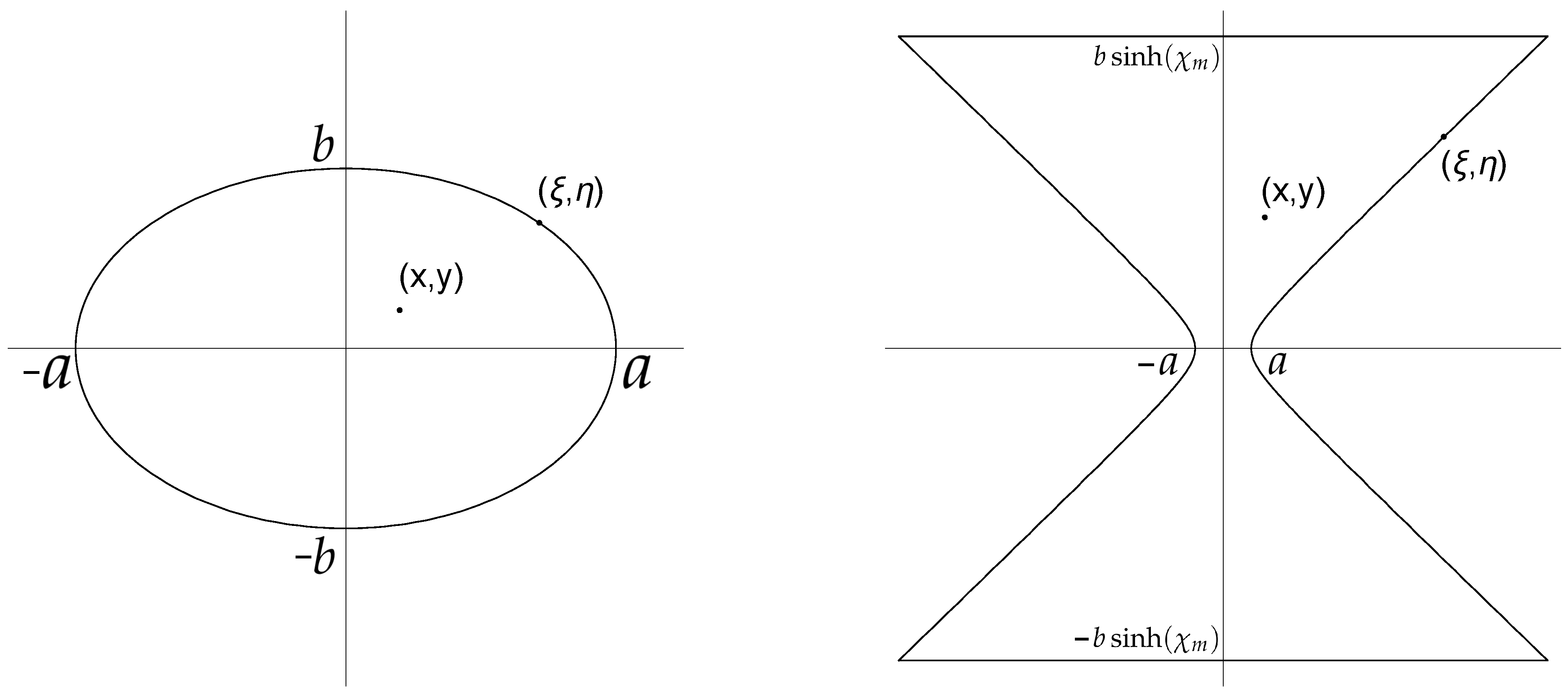
To show how the vector potential (
1) with
can be created, let us consider the concave solenoid with two hyperbolic boundaries,
, parametrized as
and
. As the current must flow along the closed circuit, we suppose that
, so that the circuit is closed by two straight lines
. In this geometry, the component
is determined only by the current in the hyperbolic boundaries. It can be written as (if the current flows in the counterclockwise direction)
In the linear approximation, with respect to variables
x and
y, we arrive at the integral
This integral can be calculated exactly [
19]. The result is
If , then is close to the unity. But can be less than for sufficiently large values of parameter . In particular, if and , then .
The linear approximation for the vector potential can be justified if the transverse solenoid size is much larger than the Larmor radius of the charged particle . For the quantum particle with the minimum energy , one has . To have an idea on the orders of magnitude of parameters, we consider an electron moving in a magnetic field of order of G. Then, s and cm. Therefore, the linear approximation is quite good for solenoids whose transverse dimensions are much bigger than mm and magnetic fields are stronger than G.
3. Main Equations
We consider a quantum nonrelativistic spinless particle of mass
m and charge
e, whose motion in the
plane is governed by the Hamiltonian
If the magnetic field
does not depend on time, then Hamiltonian (
17) admits two linear integrals of motion,
which are merely the coordinates of the center of a circle, which the particle rotates around with the cyclotron frequency
. The importance of these integrals of motion was emphasized by many authors during decades [
4,
17,
20,
21,
22,
23,
24,
25].
The second pair of physical observables consists of two relative coordinates:
Then Hamiltonian (
17) with
can be written as
Due to the commutation relations,
the eigenvalues of operator (
20) assume discrete values
. Moreover, these eigenvalues have infinite degeneracy [
4], because they do not depend on the mean values of operators
and
(or their functions). In addition to the energy, there exists another quadratic integral of motion, which can be considered as the generalized angular momentum (the formulas below are identical for the classical variables and quantum operators; therefore, we do not put here the symbol
over operators):
It coincides formally with the canonical angular momentum
in the case of “circular” gauge of the vector potential. It follows from (
22) that the “kinetic” angular momentum, defined as
is not a conserved quantity, and it can vary with time in the generic case [
20,
26,
27]. On the other hand, the “intrinsic” angular momentum
is obviously conserved for the constant magnetic field. Formulas (
22) and (
23) can be written in terms of “geometric” variables (different from the phase plane coordinates) as
It is convenient to use the vector
, whose components can be either classical variables, quantum operators, or mean values of these operators. The initial values, before the variation of parameters, are contained in vector
. Vector
contains the information about the geometrical coordinates after the variations of parameters. Due to the linearity of the equations of motion, these two vectors are connected by means of some transformation matrix
:
Here, are four blocks of the matrix .
The mean energy in the stationary magnetic field equals
. It can be written as the sum of two independent parts:
where
with
. The quantity
coincides with the energy of the classical particle moving along the mean trajectory
, whereas the quantum correction
in (
27) arises due to quantum fluctuations, described by means of the variances
and
of the relative coordinates.
3.1. Change of the Classical Part of Energy
The change of the classical part of the mean energy can be written as some quadratic form with respect to the initial quantum-mechanical mean values of the relative and guiding center coordinates:
, where coefficients
are certain bilinear combinations of the elements of matrix
. Therefore,
depends on four initial parameters. In particular, these parameters can be almost always chosen in such a way that the final classical part of energy will be equal to zero. For example, it is sufficient to solve the equations
with respect to the initial values
and
with fixed values of
and
. The answer in terms of elements of matrix
is as follows,
However, this is an extremely peculiar situation.
Therefore, let us consider a rarefied gas of charges in the uniform magnetic field. Neglecting the interaction between charges (i.e., assuming the magnetic field to be strong enough), we can write the total energy as the sum of independent single-particle energies. However, the positions of guiding centers of the gas particles can be quite arbitrary, as well as the concrete values of the relative coordinates of each particle (obeying the restriction
. In such a case, the most interesting quantity is the average value of
, where the averaging is performed over the whole ensemble of charges with arbitrary initial quantum-mechanical mean values. Designating such an additional averaging by means of the over-line (to distinguish from the primary quantum-mechanical averaging), it seems natural to assume the absence of initial correlations and the isotropic distribution of non-zero mean values:
Here,
is the average square of the distance between the classical guiding center position and the center of solenoid, whereas
is the average square of the classical radius of orbit. Under these assumptions, the average change of the classical part of energy can be written as
where
and
means the transposed matrix. Coefficient
is always non-negative. However, coefficient
can be negative, thus indicating a possibility to cool the gas by means of fast variations of the magnetic field.
3.2. Change of the Quantum Part of Energy
It is convenient to combine all covariances in the single
symmetrical covariance matrix
. Then, the linear transformation (
26) implies the following relation between the final (
) and initial (
) covariance matrices [
28],
where
is the transposed matrix. The change of the quantum part of the mean energy,
depends on the evolution matrix
and the initial covariance matrix
. In general,
can have 10 independent elements (obeying some restrictions due to the uncertainty relations). Therefore, it is difficult to analyze the problem for the most general initial states. We consider the simplest situation, when the initial state possesses some rotational symmetry inside the pairs
and
. Therefore, we assume that non-zero initial elements of matrix
are
and
, i.e.,
where
is the
unity matrix. Then,
In view of the commutation relations (
21), two positive parameters in matrix (
36) must obey the restrictions
and
. In particular, the variance matrix (
36) can describe the thermal quantum state with different temperatures of the
and
subsystems. However, this is by no means the only possible state, because the covariance matrix describes uniquely only the Gaussian states (unless
).
3.3. Change of the Average Guiding Center Position
Calculations similar to that of the preceding subsections give the following formulas for the “classical” and “quantum” parts of the change of the average square of the radius of the guiding center position.
One can see that, under conditions (
30) and (
36), the formulas for the “classical” and “quantum” parts of the quantities
and
are, in fact, identical, if one makes the formal substitutions
and
(remembering that parameters
and
G are limited from below, whereas
and
can be arbitrary non-negative numbers). Therefore, in the subsequent sections, we give explicit formulas for the “quantum” parts of the quantities under study only.
3.4. Change of the Angular Momentum
Due to the choice of the initial variance matrix in the form (
36), the initial mean value of the quantum part of the angular momentum operator (
25) equals
. Equations (
25), (
34) and (
36) yield the following formula for the change of this quantity,
3.5. Evolution of the Magnetic Moment
The operator of magnetic moment
can be introduced in several ways. One can start from the thermodynamic relation
and define
. This definition was used, e.g., in [
20] for the circular gauge (
). For the general linear gauge, such a definition results in the formula
However, one can use as the starting point the standard definition of the classical magnetic moment
Then, using the expression for the quantum probability current density
one can write the right-hand side of (
42) as the mean value of operator
Therefore, the relation
does not hold for the time independent angular momentum (
22).
Formulas (
41) and (
44) coincide only for
(note that namely this special gauge was used in the overwhelming number of papers devoted to the motion of quantum particles in the magnetic field). However, writing the operator
in (
41) as
, one can see that the average value of
over the period
equals zero (as
and
do not depend on time, whereas
and
oscillate with frequency
in the Heisenberg picture; in addition, the difference
oscillates with frequency
). Using the symbol
for the double averaging (over the quantum state and over the period of rotation in the magnetic field), we have
. Moreover, in view of (
24) and (
25), we have
. Therefore,
, for any definition of the magnetic moment operator. (Actually, some authors used this formula as the definition of the magnetic moment of a charged particle moving in the magnetic field [
29].) This relation explains why different choices of the vector potential gauge do not influence the final results for the magnetization of the free electron gas in the time-independent magnetic field. Designating
, we obtain the following expression for the quantum part of the change of the magnetic moment in the nonstationary case,
3.6. The Transformation Matrix for the Sharp Jump of Parameters
For the constant magnetic field with the cyclotron frequency , the canonical coordinates are related to the “geometrical” coordinates as follows,
The canonical coordinates (or mean values of the corresponding operators in the quantum case) do not change during the instantaneous finite jump of the parameters (as the wave function cannot change instantaneously in the nonrelativistic quantum mechanics; the same result can be obtained by integrating the equations of motion for the canonical variables during the infinitesimally short time of the jump). However, the relations between the canonical and geometrical variables are different before and after the jump. Therefore, one can easily find the elements of matrix
, solving the equations
and similar equations for the pair
. If
and
, then
where
Matrix (
48) equals the unity matrix if
. For this reason, many formulas in the subsequent section have the most compact form if they are written in terms of parameter
, instead of
.
4. Results
4.1. Energy Evolution
Equations (
37), (
48) and (
49) yield the following expression for the quantum part of the energy change,
The energy always increases after the jump of the gauge parameter with the fixed value of the magnetic field (): . On the other hand, can be negative for the fixed and negative values of parameter inside the interval
The minimum is achieved in the middle of this interval:
In the special case of , we have
In this case, the quantum part of the energy can be reduced to the half of the initial value for (the circular gauge) and (the total switch off the magnetic field), but it can be reduced by only 25% for (the Landau gauge) and . For (or ), we have
Another interesting special case is (when : the instantaneous inversion of the magnetic field). Then,
For (the Landau gauge), the energy always increases, and the increase depends on the initial fluctuations of the guiding center position only. On the other hand, if , then , so that the final quantum part of energy is determined by the guiding center fluctuations: .
4.2. Shift of the Guiding Center and Variation of the Angular Momentum
The “classical” and “quantum” parts of the guiding center mean position shift are described by Equations (
38) and (
39). The explicit formula for the quantum part is as follows,
For small changes of the magnetic field, when
and
, we have
. According to (
56),
for
. However, this is a consequence of Equation (
18), because in the absence of the field the particle moves along a straight line, whose curvature radius is obviously infinite.
If but , then is always positive. A more interesting case is . For example, if , then
In this case, if , then for , whereas for , with the critical value , when changes its sign.
The angular momentum does not change its value for any values of parameters
and
, as Equation (
40) leads to the formula
. Actually, this is the direct consequence of Equations (
22), (
36) and the instant jump approximation, because the canonical coordinates do not change during the instant jump, whereas
, due to the diagonal form of the initial covariance matrix. Situations with
can happen for asymmetric initial conditions.
4.3. Change of the Mean Magnetic Moment
Using Equations (
45) and (
48), we obtain the following formula for the relative change of quantum part of the mean magnetic moment
(where
is the initial magnetic moment):
We see that the sign of change is determined completely by the sign of ratio . If , then any change of the solenoid shape increases the magnetization: .
If , then , so that the Landau gauge yields a twice bigger relative change of the magnetic moment than the circular gauge. Bigger changes can be achieved in hyperbolic solenoids with . Note that function is symmetrical with respect to the transformation . Consequently, the increase and decrease of the magnetic field result in the same relative change of the magnetic moment (by the absolute value). If (the instant inversion of the magnetic field), then , so that for and , but for the Landau gauge.
4.4. Generation of Squeezing
The squeezed states of a free charged particle moving under the homogeneous magnetic field (with the circular gauge of the vector potential) were considered by several authors [
16,
30,
31], but they calculated the squeezing coefficients with respect to the canonical pairs of variables, such as
and
, whose physical meaning is not quite clear. Therefore, it was suggested in [
32,
33,
34] to analyze the variances in the pairs
and
. The states possessing variances of any element of the pairs
or
less than
were named “geometrical squeezed states” (GSS) in [
7], to emphasize that all the observables
have the meaning of coordinates in the usual (“geometrical”) space, and not in the phase space. Only the circular gauge was considered in [
32,
33,
34]. Two gauges—the circular and Landau ones—were compared in [
7].
An interesting problem raised in [
7] is how one could create GSS, starting from coherent states (having all variances equal to
). For the single-mode systems, such a problem can be solved effectively by using quadratic Hamiltonians with suitably chosen time-dependent coefficients [
28]. However, can this can be done using time-dependent magnetic fields in two dimensions? It appeared that the answer depends on the choice of time-dependent gauge. Namely, it was shown in [
7] that no squeezing can be obtained for any geometrical observable
for an arbitrary time-dependent magnetic field described by means of the circular gauge of the vector potential. On the other hand, some degree of squeezing can be obtained in the case of Landau gauge. These observations explain our interest to the general vector potential (
1).
Let us suppose, for the sake of simplicity, that the initial state was coherent with respect to all geometrical observables, i.e., . Then, we have the following form of matrix immediately after the jump, , where
The relative squeezing with respect to the new ground state value
immediately after the jump is characterized by two coefficients:
If
, then squeezing is possible provided
. The maximum squeezing of 50% can be achieved for
. If
, then
so that no squeezing is possible for the circular gauge (
), in accordance with the authors of [
7]. On the other hand,
for
. In any case, squeezing is possible only for
. The minimal value
can be achieved for
. If
, then
, so that squeezing is possible for any
. Note the symmetry relations
and
.
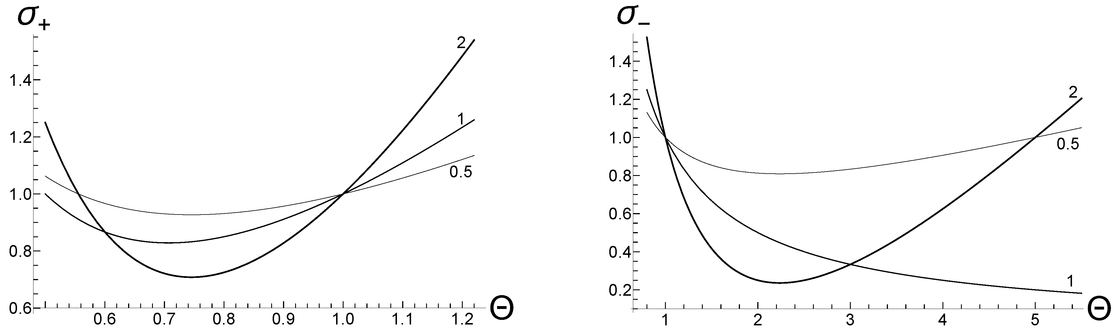
Figure 2 shows typical plots of
for some fixed positive values of
.
5. Discussion
The results of the preceding section show that, indeed, the choice of the gauge parameter (i.e., the choice of the solenoid shape) can influence significantly on changes of many physical quantities after the stepwise variation of the magnetic field. Moreover, it appears that the directions of these changes can be quite different for different quantities. For example, the change of the mean value of the angular momentum does not depend on (for the chosen symmetric initial conditions). The energy change can be stronger for the circular gauge () than for the Landau gauge with . On the contrary, no squeezing can be created from the initial coherent state for , whereas it can be quite significant for . However, the most interesting results, probably, are related to the change of the average magnetic moment.
This change is twice bigger for the Landau gauge than for the circular one. The magnetic moment increases with the increase of the magnetic field, and this behavior seems natural. An unexpected result is the increase of the magnetic moment when the magnetic field decreases. An especially strange consequence is the infinite magnetic moment after the instant switching off the magnetic field. Of course, the sharp change of the magnetic field in time is an idealization, which can be justified if the magnetic field varies rapidly during a small time interval
. This means that the particle practically does not change its position, and its wave function does not change its value, during the interval
. On the other hand, the time-dependent magnetic field in the empty space inside the solenoid cannot be strictly homogeneous, due to the time dependence of the induced electric field. However, this inhomogeneity can be neglected if the Larmor radius is much smaller than the scale of spatial variations of the time-dependent electromagnetic field, which is of the order of the characteristic wave length
. Thus, we arrive at the restrictions
, which are self-consistent if the cyclotron frequency satisfies the condition
, which is equivalent to
. For the electron, one obtains
G. Consequently, the model considered in the paper seems to be well justified for typical magnetic fields used in laboratories, which do not exceed
G (see also [
16]). For
s
(
G), the restrictions on the parameter
takes the form
s. These restrictions are much softer for atomic ions, whose masses are five orders of magnitudes higher than the electron mass.
Strictly speaking, we cannot exclude a possibility that the model of homogeneous and rapidly changing in time magnetic field can be invalid for , when the quantum Larmor radius becomes too large. This special case needs a separate detailed investigation. In this connection, it would be interesting to find solutions to the problem (approximate analytical or numerical), considering more realistic time dependencies of the magnetic field and the gauge parameter . Note, however, that μm for G, which can be considered as practically zero field if T.
Among other results, it is worth mentioning a possibility of cooling the system of charged particles by means of fast variations of the magnetic field. Actually, this is a subtle problem, because one has to take into account many other effects, such as the interaction between the charged particles in the gas, to make realistic estimations. On the other hand, the problem of interaction does not exist, e.g., for single ions in traps. In any case, it would be interesting to verify our results experimentally, using solenoids with different shapes of the cross sections.


