Contribution in Modeling of Traffic Flow, Using Bond Graph Model Approach: Translating Traffic into Bond Graph Model Variables—Case Study of the Area of Three Crossroads for the City of Sofia, Bulgaria

Abstract

The work presented in this study uses Bond Graphs to model and simulate complex urban traffic flow systems consisting of three interconnected, traffic-light-controlled crossroads with heavy traffic demand. Bond Graph models are highly versatile for modeling multi-domain systems and provide a convenient bridge between analytical representations and numerical implementations. In this paper, we exploit Bond Graph model theory and digital logic concepts to develop a structured methodology for deriving Bond Graph switching network models applied to urban traffic flow. A simple traffic-light-controlled crossroad is then modeled and analyzed. Moreover, the application of Bond Graph modeling to traffic flow, illustrated through a real case study of a street network in Sofia, Bulgaria, validates the proposed model-based approach. The obtained results demonstrate the relevance and effectiveness of the proposed Bond Graph model-based macroscopic traffic modeling framework in capturing the fundamental dynamics of traffic flow under signalized control. Beyond the specific case study considered, these results highlight the potential of the approach as a general and extensible tool for modeling more complex urban traffic networks. They open perspectives for future work aimed at assessing the flexibility, scalability, and generalization capability of the framework for heterogeneous intersections and large-scale traffic systems.

1. Introduction

This paper is based on our knowledge of Bond Graph models and the various ways a road and a switching network can be modeled into a Bond Graph environment. The challenge of traffic flow modeling using Bond Graphs is the complex nature of the Traffic Flow domain [1] and the difficult translation and quantization of traffic variables into Bond Graph model elements [2]. But even so, the research gives valuable insight intothe process of designing traffic-light-controlled intersections, using Bond Graph model switching networks, and the concept of segmentation of long roads for better in-depth analysis of the processes within the road.

Urban traffic congestion has become a major challenge in large metropolitan areas due to the increasing demand for mobility and the limited capacity of existing road infrastructures. In Sofia, recent traffic analysis reports an average congestion level of approximately 47%, with drivers losing nearly 113 h annually in rush-hour traffic conditions. Moreover, the average travel speed during peak periods decreases to nearly 17–18 km/h, while a 10 km trip may require more than 30 min during morning and evening congestion periods [3]. These observations highlight the strong impact of signalized intersections and traffic bottlenecks on global urban traffic dynamics and emphasize the importance of efficient trafficlight control and trafficflow optimization strategies.

With these considerations in mind, the present work is grounded in the classical macroscopic traffic flow modeling framework, which represents traffic as a continuum characterized by aggregated variables such as density, flow rate, and mean velocity. First-order macroscopic models, such as the Lighthill–Whitham–Richards (LWR) formulation, are widely used to describe the evolution of traffic states through conservation laws and fundamental diagrams relating flow and density [4,5]. These models provide a simplified yet physically consistent representation of traffic dynamics, capturing essential phenomena such as wave propagation, shock formation, and congestion development.

Recent developments in traffic flow theory further highlight the importance of non-linear effects, including phase transitions between free-flow and congested regimes, where system stability is governed by critical thresholds in traffic density and flow. To capture these critical boundaries under heavily saturated states, conventional macroscopic architectures frequently utilize a congestion boundary approach [6] to map the precise mechanics of regime phase transitions.

Furthermore, traffic behavior is strongly influenced by spatial characteristics of the road infrastructure, where variations in flow and geometric constraints, particularly in curved road segments, may induce instability and localized bottlenecking. Under these curved infrastructure boundaries, modeling the explicit influences of flow differences becomes vital to tracking dynamic phase stability and preventing unphysical velocity discontinuities [7].

These established conventional modeling milestones provide a strong theoretical baseline for the system representation adopted in this study. By pivoting from pure algebraic continuum mechanics to an energy-based system network, the proposed Bond Graph framework preserves the physical consistency of these aggregate phase shifts and geometric constraints within a modular, multi-domain framework.

In addition, traffic demand is not stationary and exhibits significant temporal variations, depending on the time of day, the day of the week, and calendar effects such as working days, weekends, and public holidays. These variations lead to pronounced changes in traffic intensity, including peak-hour congestion phenomena, as reported in previous studies [8]. In the present work, the primary objective is to first validate the proposed Bond Graph-based macroscopic modeling framework using a representative traffic scenario. Once this baseline validation is established, future developments will focus on extending the approach toward more advanced control strategies that explicitly account for time-dependent traffic demand, including peak-hour conditions and weekend traffic variations. This will enable the design of more adaptive and performance-oriented traffic control laws within the proposed modeling framework.

Generally, there are three graphical representation schemes prominently used for modeling engineering systems: Block diagrams, Signal Flow graphs, and Circuit diagrams. Block diagrams consist of blocks that represent transducers, interconnected by paths that represent signals. In Signal Flow graphs, a node replaces each path in a Block diagram, and each box is converted to a path; hence, it could be considered an alternative representation of Block diagrams. These two representations share the same advantages and disadvantages: they capture the computational structure of the system but do not preserve its topological structure. If a slight change in the physical system occurs, it might require that the entire computational structure be rearranged, and therefore, its corresponding diagram may change. An element in a power-flowing circuit has two variables simultaneously associated with it: one across variable (the potential v) and one through variable (the current i). In Block diagrams and Signal Flow graphs, these two variables are separated from each other, which tears down the analogy between the topological and computational structures [9]. In contrast to Block diagrams and Signal Flow graphs, which only preserve the computational structure of the system, Circuit diagrams can only reflect the topological structure, and their application is restricted to electrical systems.

On the other hand, Bond Graph models, originated by Paynter [10], are specifically designed to represent the conservation of energy. Presented here is a short introduction to Bond Graph models. Further details can easily be found upon searching, including in [9].

Energy can be transferred, stored and converted (into different forms) but cannot be dissipated. Hence, if the amount of energy is changing at a certain location, either additional energy is flowing in or some part of the initial energy is flowing out. In both cases, there exists a rate of change of energy with respect to time; this is defined as power, P(P = dE/dt). Power flow can be expressed as the product of two variables: an extensive variable (proportional to the amount) and an intensive variable (independent of the amount). In an electrical system, for instance, the power is a product of voltage and current: P = U × I.

The aim of this study is to research the possibilities of applying Bond Graphs as a modeling method to the traffic flow domain and possibly finding a way to implement control functions within the model. The study is based on the core principles of traffic flow theory and was inspired by many different Bond Graph model research documents dealing with the traffic flow domain or other physical domains like electricity, hydraulics or mechanics.

The study will give an overview of Bond Graph modeling methodology, as well as the established practice of translating traffic flow theory terms into possible Bond Graph model representations.

The work begins with a few simple assumptions about the traffic flow and by building simple models, starting with a physical model, transitioning into a mathematical approach and later solving possible problems using simulation software (such as MATLAB/SIMULINK, Symbols, 20Sim and Dymola). The models will gradually get increasingly complex until we end up with a small city network section consisting of traffic-light-controlled crossroads.

The paper is organized into the following sections: Section 2 introduces the design process for a traffic light using the Bond Graph method and cellular automata (based on the concept of a switching network). This section also gives an example with a relatively standard four-way crossroad with a separate traffic light section, represented as a Karnaugh map and an electrical switching network. The section ends with a validation of the obtained Bond Graph model for that traffic-light-controlled crossroad. In the following Section 3, we discuss the modeling of a more complex macroscopic model of traffic flow with energy conservation. The macroscopic model defines a relationship among traffic density, average velocity, and traffic flow. The traffic density is defined as the number of vehicles per kilometer and per lane, while the traffic flow (or the traffic intensity) is defined as the number of vehicles passing a certain point per hour. One of the main contributions of this paper is the translation of the traffic flow parameters into Bond Graph model components, and the application of some control using the presented Bond Graph model traffic light control part. The deterministic dynamic traffic Bond Graph model is a novel instrument for the analysis of traffic conditions.

Then, Section 4 presents the use of the more complex traffic flow Bond Graph approach (discussed in Section 3) to build a model of a larger city area, part of the busy street network of Sofia, Bulgaria. It consists of three consecutive multi-lane crossroads with a complex traffic light control system. Finally, in Section 5, we discuss the conclusions and perspectives of this work and the Bond Graph-based modeling approach for traffic flow control applications.

2. Designing Bond Graph Model Traffic Lights

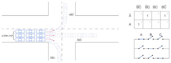
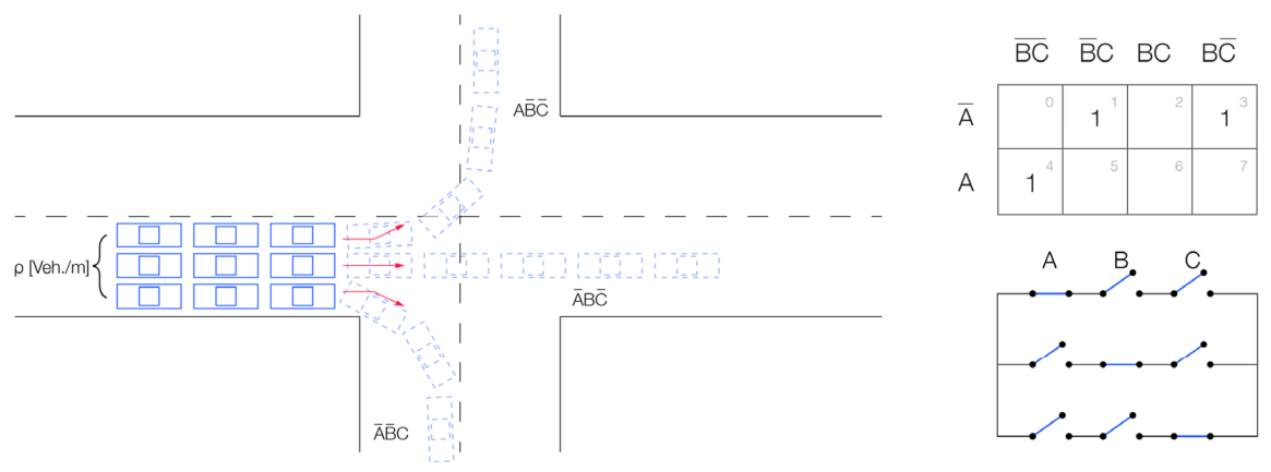
To avoid congestion and bottlenecks, especially arising in rush hours, traffic flow control in urban areas is mostly organized using traffic lights. Using Boolean algebra, we can build a model for a switching network, representing a traffic light. We can use a structured algorithm for deriving switching networks in Bond Graph models [11,12,13,14]. Considering, for example, a simple hypothetical four-way traffic-light-controlled intersection with a focus on one branch only, where the traffic light has three sections controlling the flow and going to any of the respective other three branches of the crossroad (no U-turns are allowed), as described in Figure 1, the initial conditions are as follows:

Figure 1. Simple crossroad with separate traffic light sectionsfor every direction (left) and Karnough map and electrical switching network for this 4-way crossroad (right).

• Only one section (lane) has a green light and is allowed to go at any given time;all other sections (lanes) have a red light (a switching network with “mutual exclusivity” functionality).
• One switch of one branch is closed (operating) at each time (if the cars are making a left turn, then the cars from the same branch cannot go straight across or right at the same time).

For this example, the cellular automation model describes the road as a network of connected “cells”. It is a macroscopic traffic flow model with a relation between the traffic density, the average velocity, and the traffic flow [15,16]. The continuous traffic models are too complicated to solve analytically, especially if the size of the considered traffic network is large; they are discretized in time (for example, stretches of 500 m) and space (15 s time intervals) in order to simulate their behavior on a computer.

The figure below represents that branch of the crossroad, where the theoretical traffic light model with three sections would have the following logical representation:

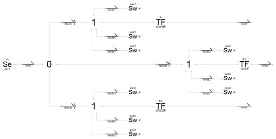
Prior evaluations of this intersection topology established baseline configurations for the switching framework before and after mitigating structural causal conflicts generated by discrete control components. As illustrated in the initial structural map (Figure 2), the switching logic is mapped using a series of 1-junctions, where each distinct directional lane array interfaces directly with a collection of three independent ideal switch elements (Sw).

Figure 2. Three-section traffic light switching Bond Graph model without solved indeterminacy. Legend: e—effort, f—flow.

However, simulating a condition in which multiple parallel switches are simultaneously set to an open-circuit state restricts the system matrix, leading to an algebraic loop or a voltage singularity that halts numerical integration. To guarantee numerical solvability across all phase transitions, the ideal switch boundaries must be relaxed by introducing parasitic elements—specifically, a supplementary high-impedance value applied to the off-state equations. That way, they become physically consistent, non-ideal switching representations.

For instance, let us take a closer look at a real-world example, where switching is “non-ideal”: If we take a traffic light with only two states (red and green), the process of switching between the two states might be practically immediate for the light, but it is not so immediate for the cars. The drivers need time to process the visual information of the changing light and act accordingly. In the case of switching to “red”, some of them, who are already too close to the stop line at the time of the change, will still choose to pass rather than jump on the brakes. Other drivers behind them will gradually decrease speed. On theother hand, it takes time for drivers to accelerate their cars to the average, or steady-state, speed of going through the crossroads.

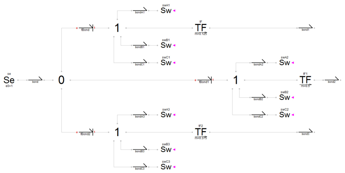
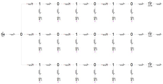
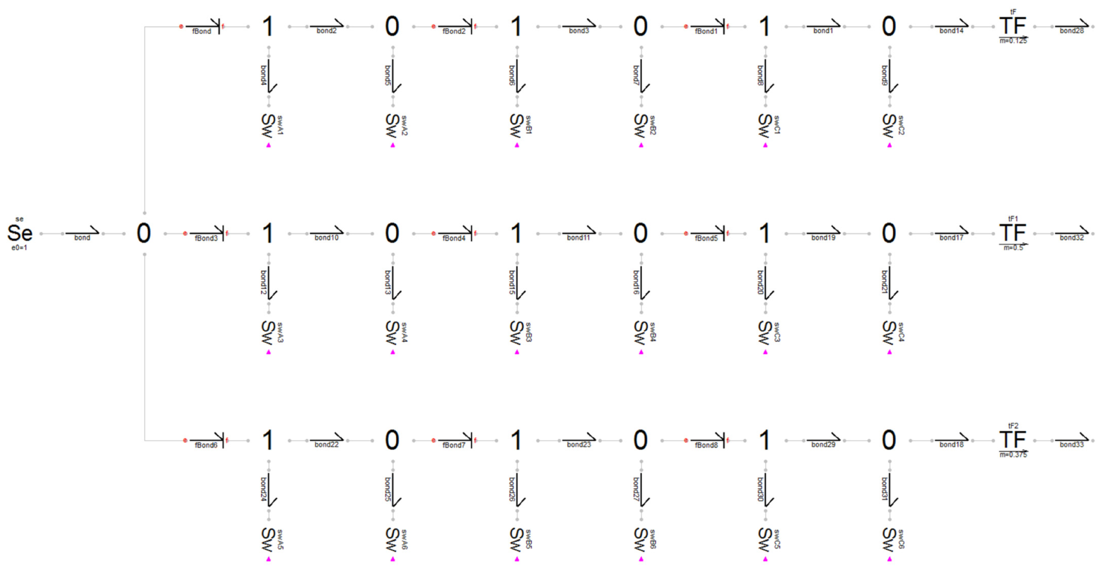
In the Bond Graph model diagram depicted in Figure 3, the type 1 junction, with three switch harpoons in each power path (from the initial model in Figure 2), has been divided into three type 1 junctions with three type 0 junctions inserted between them. In this case, each type 1 junction will have only one output bond for a single switch, and another bond towards a neighboring type 0 junction. Departing from each type 0 junction is not only the bond to the next type 1 junction but also a bond towards a newly introduced switch, which operates inversely with respect to the preceding switch connected to the type 1 junction. This newly introduced switch is responsible for guiding the residual effort towards the ground. The C-element connected to the first 0-junction represents the traffic light queue, and the C-elements at the ends of the three branches are to be considered as sinks to capture the traffic pouring in the different directions of the crossroad. Also, the coefficients of transformation of the three TF-elements sum up to 1 and are effectively being used to account for the different number of vehicles choosing to go in that direction of the crossroad.

Figure 3. Three-section traffic light Bond Graph model with solved indeterminateness and added switching control and passive elements.

3. Translating Traffic into Bond Graph Model Variables

Traditional urban mobility frameworks predominantly capture macro-regime variations through stochastic formulations and probabilistic distribution matrices. Conversely, this methodology isolates the underlying macroscopic continuum mechanics from structural disturbances by defining a strictly deterministic state-space architecture for the core traffic dynamics.

The stochastic fluctuations and driver behavioral variability are separated from the baseline conservation laws and reintroduced independently via a modulated potential field function. By utilizing this structural bifurcation, the deterministic Bond Graph framework serves as a mathematically robust diagnostic instrument to map aggregate vehicular behavior under varying environmental potential field profiles [11,15,16,17,18,19].

The proposed approach is intentionally based on the first-order macroscopic LWR (Lighthill–Whitham–Richards) traffic flow model, which represents traffic dynamics using aggregated variables such as traffic density, mean speed, and flow. In this framework, the traffic stream is treated as a compressible continuum, allowing the development of a simplified yet physically consistent representation suitable for Bond Graph modeling and energy-based system analysis.

Consequently, individual driver behaviors, such as acceleration/deceleration patterns, reaction times, aggressive or conservative driving habits, and lane-changing maneuvers, are not explicitly represented in the current model. These microscopic effects are implicitly embedded in the empirical fundamental diagram relating density and flow. The objective of this first contribution is primarily to establish and validate a Bond Graph-based macroscopic modeling framework for road traffic systems using the classical LWR formulation.

This choice provides several advantages, including reduced computational complexity, easier physical interpretation, and a unified representation of traffic propagation phenomena such as congestion waves and flow conservation. Moreover, it constitutes a solid foundation for integrating more advanced traffic dynamics in future developments.

In a busy city traffic system, vehicles are assumed to be moving as a group. The proposed macroscopic approach models complex systems, with energy conservation being one of the major principles [20,21,22].

As every bond involves two power variables, the decision on setting the cause variable and the effect variable must follow the natural laws. This has a significant bearing on the resulting state equations of the system. Proper assignment of energy direction resolves the sign-placing problem when connecting sub-model structures. The causality will dictate whether a specific power variable is a cause or the effect [18,19].

To formalize the energy conservation framework within the macroscopic LWR model, traffic streams are treated as a compressible fluid continuum. Here, vehicular density gradients generate a localized transport potential that drives the aggregate mass along the road network [23,24]. Additional elements to consider are the source element, storage and dissipative elements, kinetic and potential storage elements, and road junctions (types 0 and 1) as analogs of the physical phenomenon of traffic flow.

Table 1 presents the correspondence between the principal Bond Graph variables and their associated macroscopic traffic flow terms, together with their physical interpretation within the proposed modeling framework. This representation establishes the conceptual bridge between the energy-based Bond Graph formalism and the aggregated traffic flow variables, including traffic density, flow rate, vehicle accumulation, and traffic propagation dynamics, that are used to describe the evolution of urban traffic systems.

Table 1. Physical interpretation of Bond Graph elements in the proposed traffic flowmodeling framework.

Bond Graph Concept	Symbol	Associated Traffic Term	Proposed Interpretation
Effort variable	$e_T$	Transport Potential (TP)	Represents the transport potential associated with congestion and vehicle density differences between road sections.
Flow variable	$f_T$	Traffic flow rate	Represents the number of vehicles moving through a road segment per unit time [Veh/s].
Resistive element	R	Road resistance	Models flow limitations caused by road geometry, curvature, lane reduction, or traffic disturbances.
Capacitive element	C	Vehicle accumulation capacity	Represents vehicle flow compression within the road segments and intersections.
Inductive element	I or L	Traffic inertia (momentum lag)	Describes delayed vehicle acceleration/deceleration and gradual traffic propagation dynamics.
Source element	Se, Sf	Traffic demand input	Represents external traffic demand entering the network.
0-junction	—	Flow conservation node	Models merging/diverging traffic flows while conserving vehicle quantity.
1-junction	—	Common-flow propagation	Represents traffic propagation along connected road sections with identical flow conditions.
Modulated transformer	MTF	Downstream flow interaction	Captures the influence of downstream traffic states on upstream vehicle movement.

3.1. Modeling of Source

To construct a unified energy-conservation model within the macroscopic LWR continuum, the aggregate traffic stream is mapped using mass-transport and continuum fluid dynamics principles. Rather than tracking discrete components, the volumetric throughput (defined as the spatial vehicle flux—$f_T$, passing a fixed point per unit time), functions as the generalized flow variable

$${\mathrm{f}}_{\mathrm{T}}=\mathrm{q}\left[\mathrm{V}\mathrm{e}\mathrm{h}./\mathrm{s}\right],$$

(1)

The driving mechanism behind this flux is defined as the Transport Potential (TP), which represents the localized pressure gradient or transport potential difference between sequential road segments. The unit of TP would then be (2)

$${\mathrm{e}}_{\mathrm{T}}=\mathrm{T}\mathrm{P}\left[{\displaystyle \frac{\mathrm{J}}{\mathrm{V}\mathrm{e}\mathrm{h}.}}\right],$$

(2)

Respectively, ($e_T$, $f_T$) are defined to be the effort and the flow variables in the traffic energy domain. It can be noted that the product of effort and flow is power in watts [W], as given in the dimensional Equation (3):

$$\mathrm{Power}={\mathrm{f}}_{\mathrm{T}}.{\mathrm{e}}_{\mathrm{T}}\hspace{0.33em}\to \hspace{0.33em}\left[{\displaystyle \frac{\mathrm{V}\mathrm{e}\mathrm{h}.}{\mathrm{s}}}\right].\left[{\displaystyle \frac{\mathrm{J}}{\mathrm{V}\mathrm{e}\mathrm{h}.}}\right]=\left[{\displaystyle \frac{\mathrm{J}}{\mathrm{s}}}\right]=\left[\mathrm{W}\right],$$

(3)

According to the general Bond Graph modeling methodology, the energy conservation principle is not violated, and we have $Se=e_T$ and $Sf=f_T$.

To evaluate this dynamic mapping across an urban zone, consider the macroscopic network linking separate demographic nodes, such as a high-density residential perimeter and a commercial–industrial core. The boundary condition driving this link is treated as a non-stationary, diurnally periodic effort source ($Se$).

During late-night periods, the transport potential peaks within the residential sector are due to structural vehicle concentration. As the morning mobilization interval begins, this regional potential drops as the aggregate mass discharges into the transit corridors, pushing the volumetric flux to its maximum peak. By midday, the localizeddensity shifts entirely to the industrial destination, resulting in a negative potential gradient relative to the origin. This gradient reverses during the evening return interval, generating a positive potential peak as the mass returns to its initial boundary state (Figure 4).

Figure 4. Traffic concept, representing a residential and industrial area with an interconnecting road (left) and conceptual variation in traffic potential difference between residential and industrial area over a 24 h period (right).

3.2. Modeling Impedance and Dissipation-

Spatial throttling and energy dissipation within a transit corridor are governed by a road resistance parameter (R) that aggregates flow limitations caused by lane narrowing, speed-control infrastructure, localized bottlenecks, and surface roughness. Geometrically, the impedance factor is inversely proportional to the section width; expanding the physical lane capacity directly minimizes the structural drag coefficient of the section. Thus, the road resistance would be (4)

$$\begin{array}{l}\left\{\begin{array}{l}\mathrm{R}\approx {\displaystyle \frac{1}{\mathrm{\delta }\mathrm{n}}},\hspace{0.33em}\left\{\begin{array}{l}\mathrm{\delta }=1\hspace{0.33em}\mathrm{i}\mathrm{f}\hspace{0.33em}\mathrm{i}\mathrm{d}\mathrm{e}\mathrm{a}\mathrm{l}\hspace{0.33em}\mathrm{r}\mathrm{o}\mathrm{a}\mathrm{d}\\ \mathrm{\delta }<1,\hspace{0.33em}\mathrm{otherwise}\end{array}\right.\\ \mathrm{R}={\displaystyle \frac{{\mathrm{e}}_{\mathrm{T}}}{{\mathrm{f}}_{\mathrm{T}}}}\hspace{0.33em}\to \hspace{0.33em}\left[{\displaystyle \frac{\raisebox{1ex}{$\mathrm{J}$}\!\left/ \!\raisebox{-1ex}{$\mathrm{V}\mathrm{e}\mathrm{h}.$}\right.}{\raisebox{1ex}{$\mathrm{V}\mathrm{e}\mathrm{h}.$}\!\left/ \!\raisebox{-1ex}{$\mathrm{s}$}\right.}}\right]=\left[{\displaystyle \frac{\mathrm{J}.\mathrm{s}}{\mathrm{V}\mathrm{e}\mathrm{h}{.}^{\mathrm{2}}}}\right],\end{array}\right.\end{array}$$

(4)

The flow rate q [Veh./s] (5) can be acquired by monitoring the traffic during the entire period of the day and then averaging. The work done in moving a vehicle over a distance L is the traffic potential difference.

$$\mathrm{TMF}=\mathrm{m}{\displaystyle \frac{\mathrm{d}\mathrm{V}}{\mathrm{d}\mathrm{t}}}\mathrm{L},\hspace{0.33em}\left[\mathrm{J}/\mathrm{Veh}.\right]\hspace{1em}\left\{\begin{array}{l}\mathrm{m}-\mathrm{mass}\hspace{0.33em}\mathrm{of}\hspace{0.33em}\mathrm{the}\hspace{0.33em}\mathrm{vehicle},\hspace{0.33em}\left[\mathrm{kg}\right]\\ \mathrm{L}-\mathrm{distance}\hspace{0.33em}\mathrm{travelled},\hspace{0.33em}\left[\mathrm{m}\right]\\ \mathrm{V}-\mathrm{velocity},\hspace{0.33em}\left[{\displaystyle \frac{\mathrm{m}}{\mathrm{s}}}\right]\end{array}\right.,$$

(5)

For the resistance element, the effort and flow causal relation is presented in (6).

$$\left\{\begin{array}{l}{\mathrm{f}}_{\mathrm{T}}={\displaystyle \frac{{\mathrm{e}}_{\mathrm{T}}}{\mathrm{R}}}\hspace{0.33em}-\hspace{0.33em}\mathrm{effort}\hspace{0.33em}\mathrm{causal}\\ {\mathrm{e}}_{\mathrm{T}}={\displaystyle \frac{{\mathrm{f}}_{\mathrm{T}}}{\mathrm{R}}}\hspace{0.33em}-\hspace{0.33em}\mathrm{flow}\hspace{0.33em}\mathrm{causal}\end{array}\right.,$$

(6)

3.3. ModelingMomentum Lag and Inertia

The kinetic storage element (L) characterizes the momentum preservation and transient inertia of the moving vehicular mass. This parameter dictates the relaxation time required for an aggregated stream to alter its velocity profile. While present across all sections, this momentum lag is most pronounced along high-curvature geometries (e.g., sweeping ramps or winding roads), where vehicular streams cannot instantaneously alter their velocity profiles. When an intersection boundary condition interrupts the flow, this inertia prevents instantaneous velocity changes, enforcing smooth, physically consistent deceleration gradients.

The aggregate traffic stream possesses a distinct spatial momentum. An intrinsic delay occurs when trying to accelerate a highly dense stream from a state of stagnation, requiring a temporary surge in the local transport potential gradient. Once the stream transitions into a stabilized velocity profile, the effort required to preserve this steady flux drops significantly.

Consequently, when an intersection control variable shifts to a permissive ‘green’ state, the volumetric flow rate cannot scale instantly. Instead, it responds asymptotically as the stream overcomes its structural inertia and reaches a steady-state velocity profile that matches the downstream capacity. And of course, it will all depend on the dimensions of the road, like length, width (number of lanes), and curvature (7):

$$\hspace{1em}\left\{\begin{array}{l}\hspace{1em}\hspace{1em}\mathrm{I}\hspace{0.33em}\mathrm{o}\mathrm{r}\hspace{0.33em}\mathrm{L},\hspace{1em}{\displaystyle \frac{1}{\mathrm{Road}\hspace{0.33em}\mathrm{Width}}}\\ \mathrm{I}={\mathrm{e}}_{\mathrm{T}}{\displaystyle \frac{\mathrm{d}\mathrm{t}}{\mathrm{d}{\mathrm{f}}_{\mathrm{T}}}}\hspace{0.33em}\to \hspace{0.33em}\left[{\displaystyle \frac{\mathrm{J}}{\mathrm{Veh}.}}{\displaystyle \frac{\mathrm{J}\mathrm{s}}{\frac{\mathrm{Veh}.}{\mathrm{s}}}}\right]=\left[{\displaystyle \frac{\mathrm{J}.{\mathrm{s}}^2}{\mathrm{Veh}{.}^2}}\right]\\ \left\{\begin{array}{l}{\mathrm{f}}_{\mathrm{T}}={\displaystyle \frac{1}{\mathrm{I}}}{\displaystyle \int {\mathrm{e}}_{\mathrm{T}}\mathrm{d}\mathrm{t}-\mathrm{effort}\hspace{0.33em}\mathrm{causal}}\\ {\mathrm{e}}_{\mathrm{T}}=\mathrm{I}{\displaystyle \frac{\mathrm{d}{\mathrm{f}}_{\mathrm{T}}}{\mathrm{d}\mathrm{t}}}-\mathrm{flow}\hspace{0.33em}\mathrm{causal}\end{array}\right.\end{array}\right.,$$

(7)

3.4. Modeling of Compressibility Elements

The compressibility and boundary accumulation element (C) represents the spatial vehicle accumulation limits of a specific segment configuration. It defines the maximum boundary density a section can accommodate before reaching complete saturation. For example, when a signaling switch shifts to a closed (red) state, the downstream flux drops to zero, forcing approaching vehicles to form a queue. This local accumulation compresses the stream, causing a rapid escalation in the regional transport potential ($e_T$) across the intersection boundary (8).

$$\left\{\begin{array}{l}\hspace{1em}\mathrm{C}-\mathrm{road}\hspace{0.33em}\mathrm{width},\mathrm{parking}\hspace{0.33em}\mathrm{space},\mathrm{traffic}\hspace{0.33em}\mathrm{lightque}\\ \mathrm{C}={\mathrm{f}}_{\mathrm{T}}{\displaystyle \frac{\mathrm{d}\mathrm{t}}{\mathrm{d}{\mathrm{e}}_{\mathrm{T}}}}\hspace{0.33em}\to \hspace{0.33em}\left[{\displaystyle \frac{\mathrm{Veh}.}{\mathrm{s}}}{\displaystyle \frac{\mathrm{s}}{\frac{\mathrm{J}}{\mathrm{Veh}.}}}\right]=\left[{\displaystyle \frac{\mathrm{Veh}{.}^2}{\mathrm{J}}}\right]\\ \left\{\begin{array}{l}{\mathrm{f}}_{\mathrm{T}}=\mathrm{C}{\displaystyle \frac{\mathrm{d}{\mathrm{e}}_{\mathrm{T}}}{\mathrm{d}\mathrm{t}}}-\mathrm{effort}\hspace{0.33em}\mathrm{causal}\\ {\mathrm{e}}_{\mathrm{T}}={\displaystyle \frac{1}{\mathrm{C}}}{\displaystyle \int {\mathrm{f}}_{\mathrm{T}}\mathrm{d}\mathrm{t}}-\mathrm{flow}\hspace{0.33em}\mathrm{causal}\end{array}\right.\end{array}\right.,$$

(8)

3.5. Modeling of Road Junction

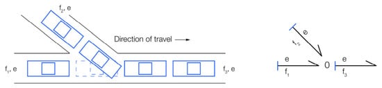
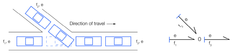
A traffic junction with no signaling is modeled as a simple 0-junction, as shown in Figure 5. The vehicles from Road 1 and Road 2 flow into Road 3, satisfying the conservation of vehicles. Thus, the algebraic sum of the flow is zero at the node, as given by the flow law (9).

$$\left\{\begin{array}{l}\mathrm{f}+{\mathrm{f}}_1+{\mathrm{f}}_2+{\mathrm{f}}_3=0\\ \mathrm{e}-\mathrm{effort}\hspace{0.33em}\mathrm{is}\hspace{0.33em}\mathrm{identic}\hspace{0.33em}\mathrm{for}\hspace{0.33em}\mathrm{each}\hspace{0.33em}\mathrm{road}\end{array}\right.,$$

(9)

Figure 5. Conjoining roads scheme and the respective Bond Graph model representation, using a 0-junction.

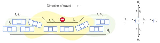
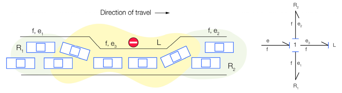
All elements on the 1-junction have the same flow and so satisfy the effort law. If we consider a narrowing in the road, it can be modeled as a kinetic storage element and a road resistor. From the principle of conservation of vehicles, the flow rate will be the same throughout the road, and the TP (transport potential) across the road will be the sum of the transport potential through the kinetic storage element L and the road resistances R1 and R2 (10), as shown in Figure 6.

$$\left\{\begin{array}{l}\mathrm{e}+{\mathrm{e}}_1+{\mathrm{e}}_2+{\mathrm{e}}_3=0\\ \mathrm{f}-\mathrm{flow}\hspace{0.33em}\mathrm{is}\hspace{0.33em}\mathrm{identic}\hspace{0.33em}\mathrm{for}\hspace{0.33em}\mathrm{each}\hspace{0.33em}\mathrm{road}\end{array}\right.,$$

(10)

Figure 6. Road segment and the respective Bond Graph model representation, using a 1-junction.

3.6. Road Segmentation Modeling Concept

Based on the previously discussed Bond Graph models of individual road elements, this section introduces the concept of road segmentation modeling. To accurately capture traffic flow dynamics across a lengthy roadway, it is advantageous to partition the road into shorter, sequential segments (or “cells”). This approach allows for spatial variations in traffic characteristics. For example, rather than applying a single, uniform resistance coefficient to the entire roadway, localized resistance coefficients can be assigned to each segment to reflect specific, real-world conditions.

The modeling process consists of several sequential steps. First, the optimal segment length must be determined. Next, these physical segments are quantified by translating real-life traffic variables into equivalent Bond Graph elements. Finally, each segment is constructed as an independent Bond Graph sub-model, connected such that the output of a preceding segment serves as the input for the subsequent one.

While Bond Graphs were originally developed to model dynamical systems with continuous energy or power flow (a characteristic that influenced our design of the traffic light switching network [16]), they do not inherently support hybrid or switched power systems, such as the traffic lights integrated here. Furthermore, standard Bond Graphs cannot easily implement loop-fed information to propagate data backward against the primary power flow. Consequently, when designing this segmented model, we must explicitly ensure that traffic flow information propagates bi-directionally, allowing downstream road conditions to dynamically influence upstream sources (preceding segments).

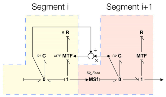
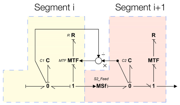
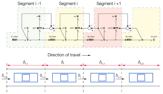
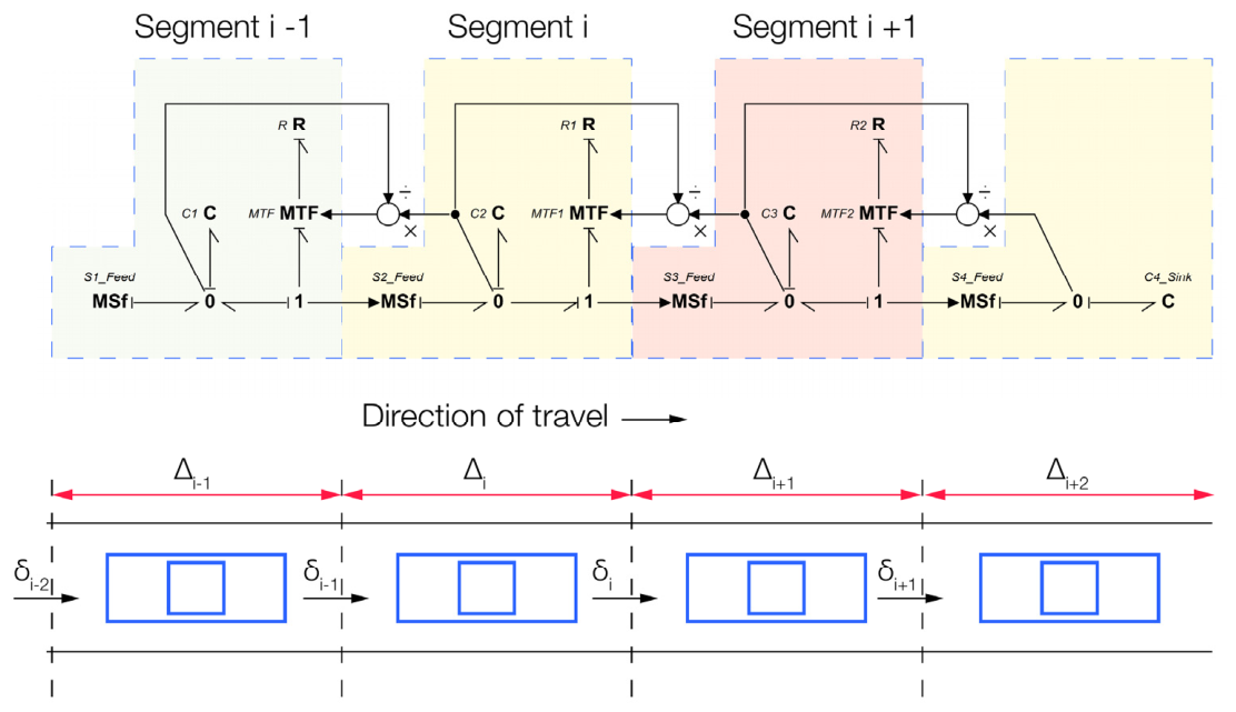
An overview of this general architectural concept is illustrated in Figure 7. The corresponding model elements depicted in Figure 7 are defined as follows:

Figure 7. Segmented Bond Graph model representation of a long road.

• C (Capacity): Represents the storage capability of the compliance (C) element, corresponding strictly to the maximum number of vehicles the ith segment can accommodate [Veh.].
• 0-junction: Ensures the conservation of the number of vehicles within the segment.
• f_T (Flow variable): Represents the average traffic flow rate in [Veh./s], defining the instantaneous number of vehicles passing a point per unit of time.
• q_T (Displacement variable): Defined by integrating the flow variable over time, representing the cumulative number of vehicles present in segment i at time t.
• e_T (Effort variable): Associated with the C-element, representing the localized vehicle density of the road segment.
• Separation Point: The boundary between adjacent segments i and i + 1, modeled by a resistance (R) element placed on a1-junction (to ensure mass conservation) and regulated by a Modulated Transformer (MTF) with a transformation coefficient μ_i.
• R (Resistance): Relates the effort to the flow, corresponding to the minimum travel time required for a vehicle to traverse segment i.
• Modulated Transformer (MTF): Integrated to account for the feedback effects of downstream traffic conditions.
• Transformation Coefficient (μ_i): Quantifies changes in driver behavior resulting from downstream traffic states. It is calibrated such that the outflow of segment i is dynamically estimated based on both the current vehicle count in segment i and the available residual capacity in the downstream segment i + 1.
• MS_f (Modulated Flow Source): Facilitates and controls the vehicle flux from one segment to the next. The MS_f preserves the anisotropic nature of traffic flow within the developed Bond Graph model, guaranteeing that vehicles can only propagate in the forward direction.

The generic Bond Graph model of a complete road section, illustrated in Figure 8, is constructed by cascading a series of the elementary Bond Graph segments previously detailed in Figure 6. Utilizing this foundational modeling framework for distinct traffic elements, alongside the multi-segment traffic behavior model (Figure 7), Section 4 presents a comprehensive case study evaluating a complex network topology.

Figure 8. Generic Bond Graph representation of a multi-segment road model, interconnected to form the entire road.

4. Case Study: Bond Graph Street Network Model in Sofia, Bulgaria

This section presents a complex, large-scale Bond Graph model of an urban traffic network. Building upon the switching network and segmentation methodologies established in the preceding sections, multiple urban intersections are integrated into a singular Bond Graph environment. The primary objective of this case study is to evaluate the efficacy of the Bond Graph framework when applied to advanced traffic control functions. Specifically, the model is analyzed regarding its numerical stability, the continuity of its state variables, and its computational efficiency (processing time) when scaling to multi-intersection topologies.

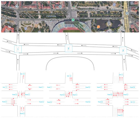
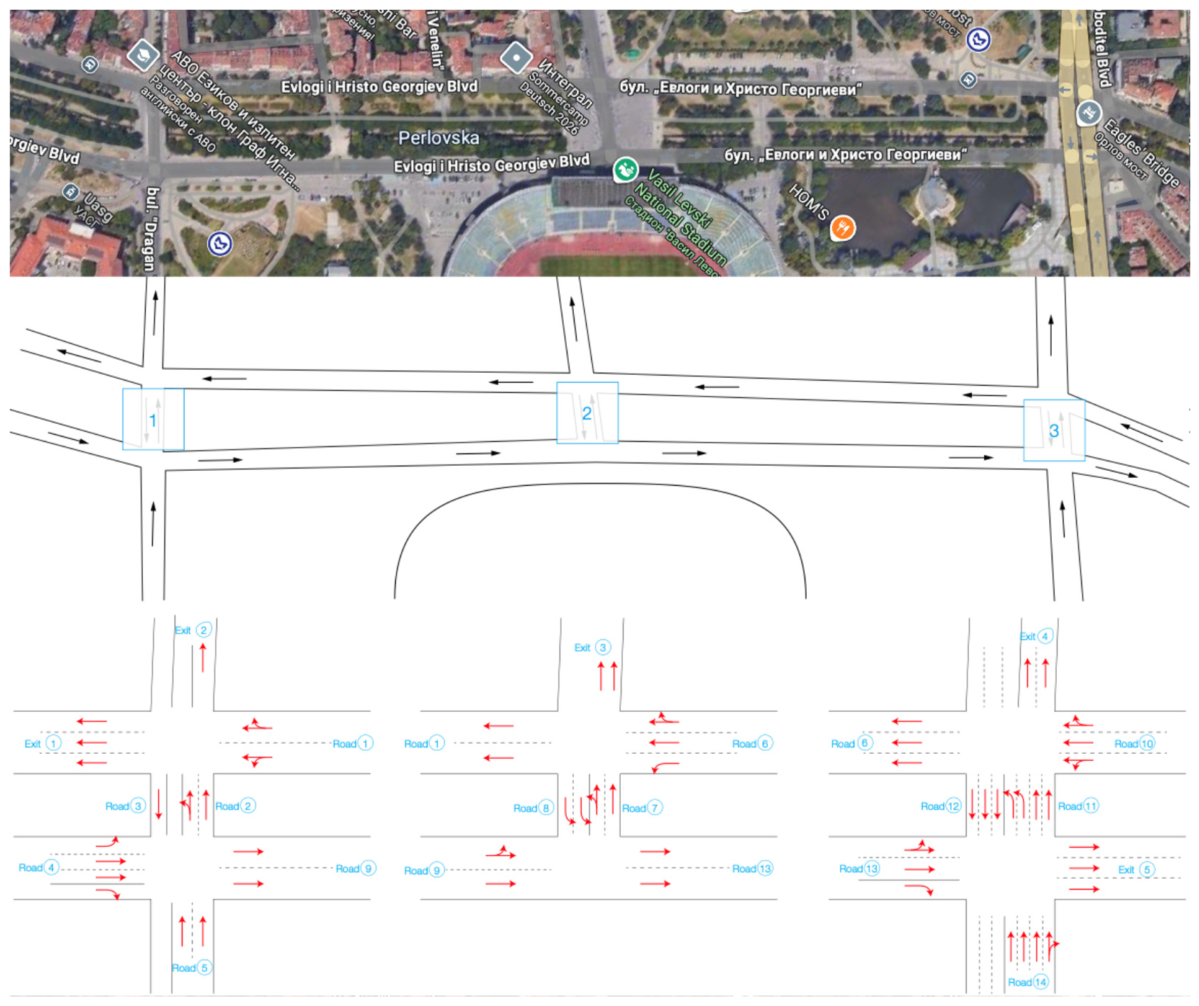
The target system for this study is a high-density urban corridor in Sofia, Bulgaria, comprising three consecutive traffic-light-controlled intersections regulating interconnected one-way arterial roads (Figure 6).

Modeling Assumptions and Simplifications

To maintain computational tractability and streamline the modeling pipeline, the following idealized boundaries and engineering simplifications were implemented:

• Lane Aggregation: Multi-lane roadways are not modeled discretely. Instead, parallel lanes are aggregated into a single macroscopic traffic stream. Bond Graph modulated transformers (MTFs) are utilized to dynamically distribute the traffic volume based on directional turning ratios.
• Boundary Condition Reduction: To minimize the number of source and sink elements (entry/exit points) at the network boundaries, specific secondary intersection branches were restricted to unidirectional flow (Figure 9). This restriction applies to Exit 2 and Road 5 at Intersection 1; Exit 3 at Intersection 2; and Exit 4, Exit 5, and Road 14 at Intersection 3.
• Idealized Signal Switching with Inertial Compensation: To establish clear mathematical boundaries for the multi-intersection switching framework, the structural signal-control configurations are explicitly categorized into included parameters and intentional engineering simplifications. Table 2 details the exact operational status of these signaling components within the macro-continuum Bond Graph architecture, alongside the physical justifications and system-theoretic impacts of each exclusion.

Figure 9. Graphical representation of the chosen part of the Sofia urban traffic network: spatial layout and intersection-level traffic modeling.

Table 2. Structural boundary matrix of signalized intersection control parameters.

Signal Component	Modeling Status	System-Theoretic Justification & Simulation Impact
Signal Component	Included	Directly implemented as the temporal period of the external binary control signal trajectories.
Protected Left-Turn Phases	Included	Modeled via directional MTF using empirical turning ratios to separate conflicting fluxes.
Yellow Change Interval	Excluded (Compensated)	Omitted from the explicit control states to prevent unnecessary matrix inflation. Instead, the gradual braking and reaction delays are implicitly absorbed by an inductive compliance (I) element, maintaining smooth macroscopic deceleration gradients without altering the core first-order LWR switching logic.
All-Red Clearance Time	Excluded	Not represented as a unique state due to the aggregate, continuous fluid nature of the macroscopic stream. Omitting this brief clearance window results in a highly conservative estimate of maximum intersection capacity, as it assumes instantaneous transition to the opposing phase.
Start/End Lost Time	Excluded (Compensated)	Merged directly into the global relaxation time constant of the junction’s inertia (I) elements. This handles the aggregate startup delay of the vehicle cluster asymptotically, ensuring realistic queue discharge without tracking single-vehicle reaction gaps.
Saturation Flow Rate	Excluded (Aggregated)	Microscopic saturation gap tracking is outside the scope of first-order continuum mechanics. The maximum discharge boundary is implicitly embedded within the empirical capacity limits (C) and the local dissipation factors (R) assigned to the intersection boundaries.
Pedestrian Phases	Excluded	Omitted because pedestrian interactions represent highly stochastic, localized microscopic disruptions. Within the macroscopic framework, these interferences are treated as stationary structural drag forces that are globally absorbed into the fixed road resistance parameter (R).

A representation of the studied traffic network and its decomposition into interconnected junctions ispresented in Figure 10. The model includes multiple intersection types within a unified Bond Graph model-based framework. In particular, Crossroad 2 corresponds to a T-road configuration, illustrating the ability of the proposed approach to represent heterogeneous junction geometries (crossroads and T-junctions) within the same macroscopic traffic modeling structure.

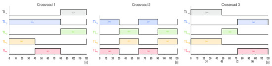
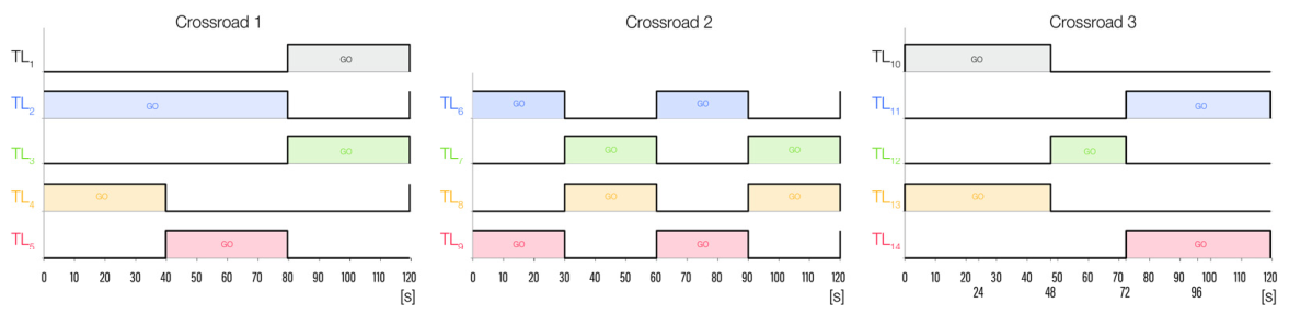
Figure 10. Traffic light control signals: TL1 (Traffic Light 1) is situated at the end of road 1, TL2 is the traffic light at the end of road 2, etc.

In this work, the traffic signal is modeled as a binary switching system composed of two dominant and stable operating states corresponding to the “green” and “red” phases. This representation is consistent with the macroscopic LWR model formulation and the switching structure of the Bond Graph model approach adopted in this work. The yellow phase is not introduced as an explicit control state. Instead, its effect is implicitly captured through an inertia (I) element, which reproduces the gradual deceleration and acceleration of vehicles near traffic lights and ensures a smooth transition between stopping and restarting phases. In this way, the inertial dynamics account for the macroscopic influence of the yellow phase on traffic evolution without requiring its explicit modeling.

From a system-theoretic perspective, the model focuses on the main macroscopic transition governing traffic evolution at an intersection, namely the alternation between a flow-transmission state (green phase) and a flow-interruption/compression state (red phase). These two regimes represent the dominant dynamics of congestion formation and dissipation.

Within this framework, the signaling process is therefore implemented as a binary switching mechanism. The yellow phase is treated as a short transient event rather than a distinct operating state, with negligible impact on the aggregated variables of the first-order LWR model. The simplified binary formulation enables a tractable and energetically consistent representation while preserving the essential switching behavior of the intersection.

The traffic light control signals for each interface are illustrated in Figure 10. To seamlessly implement the signalized intersection framework within an energy-based model architecture, the control configurations can be mathematically formulated through three alternative approaches: macro-modeling via continuous state-variable approximations, discrete ideal power switches, or boundary modulation using binary (0-1) state transformations.

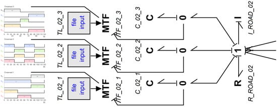
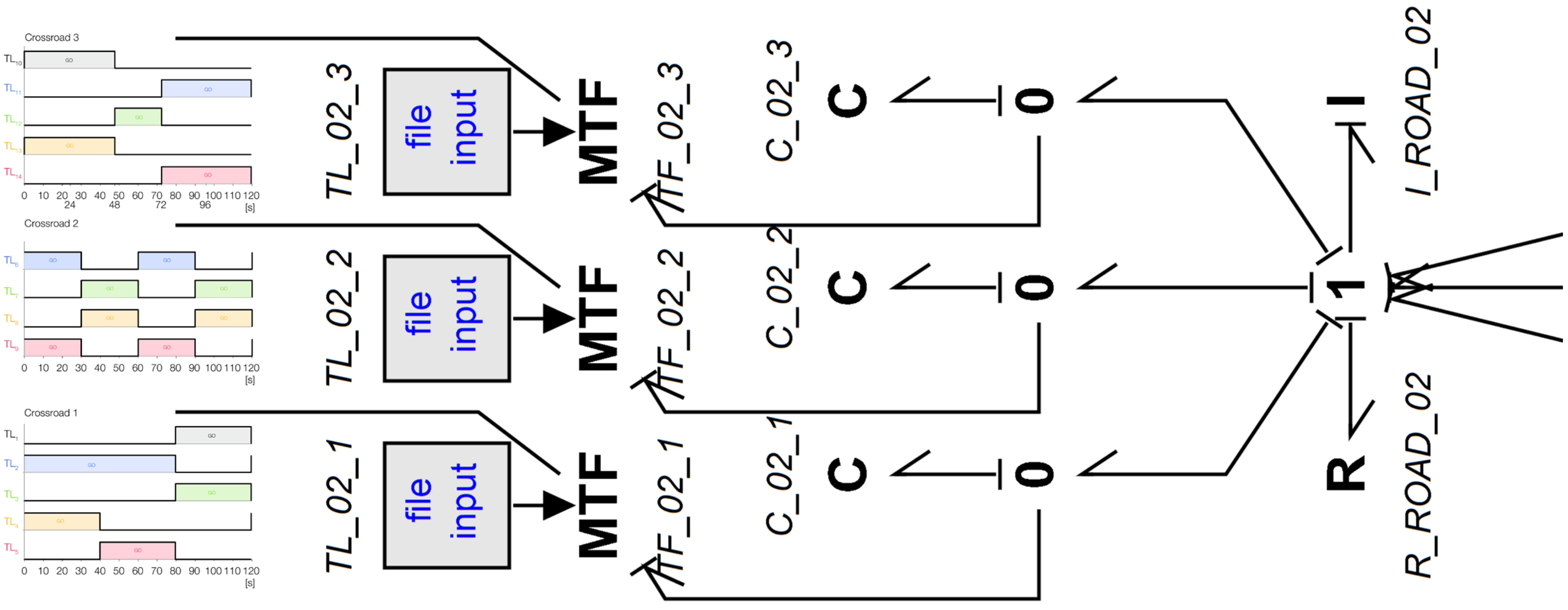
To optimize computational efficiency and minimize the dimensionality of the state-space matrix, this framework represents the network’s phase transitions using Modulated Transformers (MTFs). This methodology replaces explicit hardware switches with variable transformation coefficients that selectively scale transmission boundaries based on established control timing laws. Consequently, the number of switching elements (units) in the model corresponds exactly to the total number of distinct traffic light sections. These transformers are regulated by an external control signal (Figure 11); in this study, an empirical data-feed file is utilized to align the simulation with real-world timing patterns.

Figure 11. Three-section traffic light Bond Graph model using switching elements and control signals.

For the numerical simulation of the three-section intersection network, the traffic routing scenario is defined as follows: assuming the aggregate inlet flow entering the junction represents a normalized unity (1.0, or 100%), the directional split dictates that a volume coefficient of 0.70 (70%) executes a left turn into Road 1, a fraction of 0.25 (25%) continues straight toward Exit 3, and a minor portion of 0.05 (5%) performs a U-turn into Road 8.

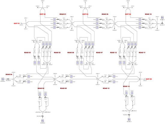
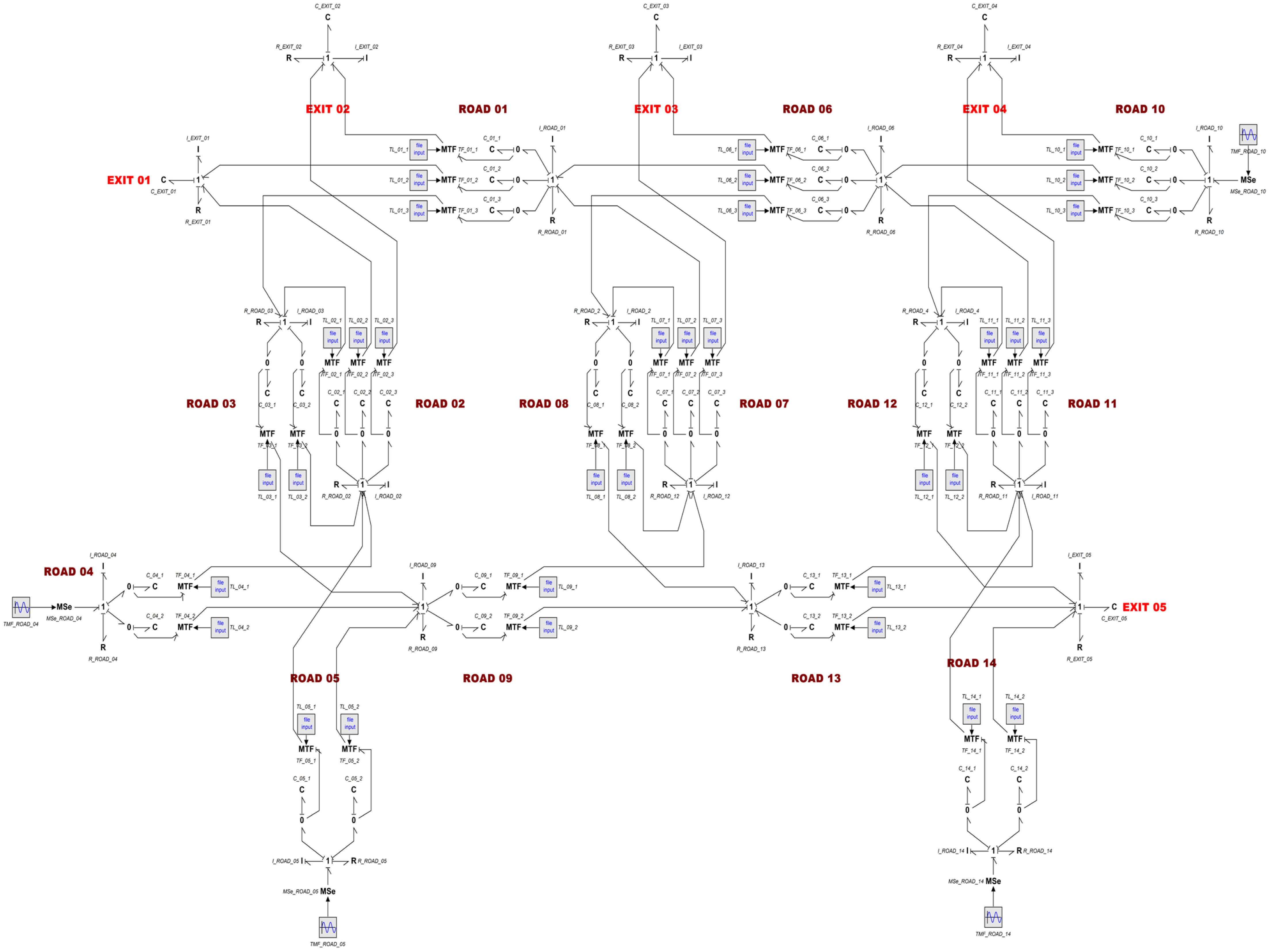
The complete Bond Graph model of the three interconnected urban intersections is illustrated in Figure 12.

Figure 12. Full Bond Graph model of the urban traffic network in Sofia. The model consists of modular road segments, intersection junctions, traffic light control subsystems (MTF-based switching), and boundary source/sink elements. The apparent complexity reflects the scalable and repetitive structure of the proposed Bond Graph formulation.

To enhance the readability of the comprehensive system architecture, the structural layout can be conceptually mapped and read via its distinct functional subnetworks. The naming convention used for elements is [element type]_[road segment]_[consecutive element].

• Road Segment Modules: Composed of compliance (C) and resistance (R) elements that capture vehicle storage capacity and localized travel times, respectively. Long segments are divided sequentially into discrete intermediate blocks (for example, for road 1, those are C_01_1, C_01_2, C_01_3, representing the three lanes of this section).
• Intersection Dynamics: Represented by standard 0-junction and 1-junction structures to ensure the conservation of vehicle volume and mass flow at junctions. The0-junctionsgovern divergent or convergent lane branches where vehicular flows divide, while the1-junctionsdictate common-flow longitudinal propagation across sequential stretches.
• Traffic Light Control Subsystems: Implemented via Modulated Transformers (explicitly marked as MTF) that selectively regulate flow transmission boundaries based on external signal timing laws. They are combined with bluefile inputlogic data-blocks (again, for road 1, those are TL_01_1, TL_01_2 and TL_01_3), which dynamically scale the boundary transmission coefficients based on the active signal timings.
• Boundary Conditions (Source/Sink Elements): Upstream input flows enter the system via the MSe (Modulated Effort Source) nodes (e.g., MSe_ROAD_04, MSe_ROAD_05, MSe_ROAD_10 and MSe_ROAD_14), while vehicles exit the network into the capacitive exit nodes (e.g., EXIT 01, EXIT 02, EXIT 03, EXIT 04 and EXIT 05).

Although the complete network diagram exhibits high topological complexity due to the large volume of interconnected elements, this architecture underscores the inherent scalability of the proposed Bond Graph formulation. Because each individual road section is modeled using a repeated, modular pattern, the framework guarantees a consistent physical interpretation across the entire macroscopic network.

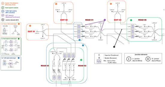
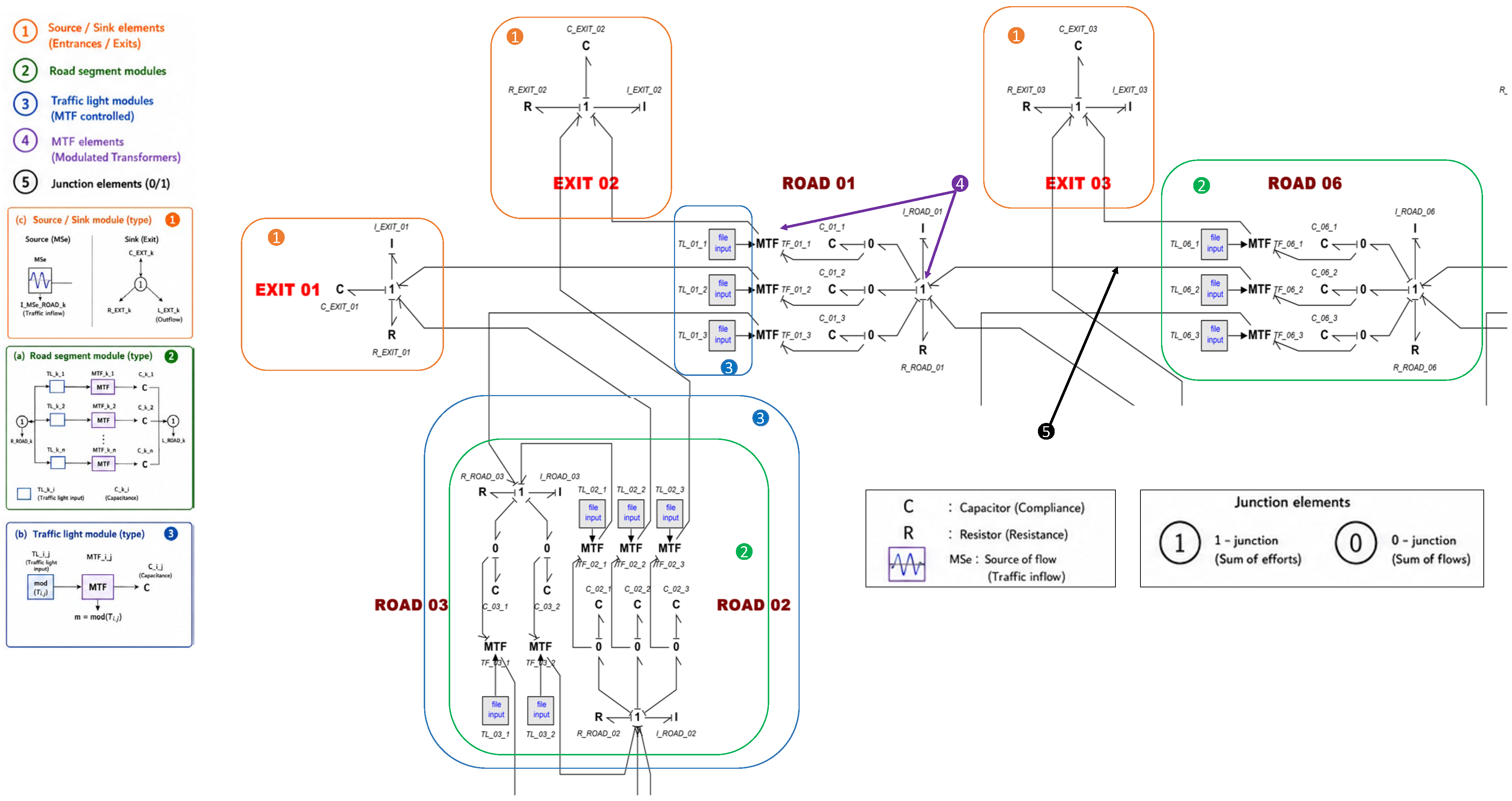
To improve the readability of the complete Bond Graph model, Figure 13 has been redesigned using highlighted regions and enlarged subfigures. The principal functional components of the network are identified using numbered annotations and colored bounding boxes. Three enlarged views are additionally provided to illustrate the most important modeling structures.

Figure 13. Annotated Bond Graph model of the Sofia urban traffic network. Numbered and color-highlighted regions identify the main functional modules of the model. Enlarged views show (a) a representative road-segment module; (b) a trafficlight control module based on Modulated Transformers (MTFs); and (c) an intersection module using 0-junction and 1-junction structures. The figure highlights the modular and scalable architecture of the proposed Bond Graph traffic modeling framework.

We present a representative road-segment module composed of storage (C), resistance (R), and modulation elements used to model vehicle accumulation, travel-time effects, and downstream traffic interactions. Moreover, we illustratea trafficlight control module implemented through Modulated Transformer (MTF) elements and associated control signals governing the switching between red and green phases. Figure 13c highlights a typical intersection structure based on 0-junctions and 1-junctions, ensuring the conservation of vehicle flow throughout the network.

The annotated representation emphasizesthe modular and repetitive architecture of the proposed Bond Graph formulation. Although the complete model contains a large number of interconnected elements, the network is constructed from a limited set of elementary building blocks, which facilitates scalability and extension to larger urban traffic systems.

Figure 14 shows the matrix of distances (in meters) for every connection (road segment) of the test area. The table clearly shows the four long segments of 350 m, representing Road 1, Road 6, Road 9, and Road 13. Table 3 shows some of the field measurements conducted, which are also the basis for the modulated transformer’s coefficients and were used in various trial models built previously.

Figure 14. Matrix of the distances [m].

Table 3. Traffic data from field observations.

Sections	Occupancy [Veh.]	Monitoring Time [s]	Flow Rate [Veh./s]	Green [s]	Red [s]	Cycle [s]
R4–E5	8	270	0.030	75	50	125
R4–R11	146	270	0.541	75	50	125
R11–E4	78	270	0.289	75	50	125
R11–R6	38	270	0.141	20	50	70
R10–E4	5	240	0.021	70	55	125
R10–R6	20	250	0.080	70	55	125
R10–R12	12	240	0.050	70	55	125
R13–R11	13	240	0.054	25	60	85
R6–E3	14	270	0.052	20	30	50
R6–R1	58	270	0.215	20	30	50
R6–R8	4	270	0.015	20	30	50
R8–R13	analytical	N/A	0.195	20	30	50
R9–R13	analytical	N/A	0.195	30	20	50
R7–R1	3	270	0.011	20	30	50
R1–E2	4	270	0.015	85	105	190
R1–R3	12	270	0.044	85	105	190
R1–E1	41	270	0.152	85	105	190
R2–E2	18	270	0.067	45	105	150
R2–E1	22	270	0.081	45	105	150
R4–R9	46	330	0.139	25	165	190
R4–R2	5	330	0.015	25	165	190
R5–R9	22	330	0.067	40	145	185
R5–R2	71	330	0.215	40	145	185

The simulation results validate the efficacy of the proposed Bond Graph framework for modeling macroscopic traffic flow dynamics alongside complex roadway geometries. Furthermore, the integration of traffic light control architectures within the Bond Graph domain successfully demonstrates how switching elements can modulate green and red waves to optimize urban traffic control.

To clarify the explicit link between empirical field observations and the proposed Bond Graph formulation, the data presented in Table 3 are mapped directly onto corresponding model components. The measured vehicle occupancy values dictate the states of the capacitive storage elements (C), representing instantaneous vehicle accumulation within each road segment. Concurrently, the observed flow rates correspond to the flow variables (f_T) in the Bond Graph domain, defining the volume of vehicles traversing a segment boundary per unit of time. The monitoring intervals establish the temporal horizon utilized for simulation and validation purposes.

Furthermore, traffic signal timing parameters, including green and red intervals and overall cycle lengths, are directly translated into binary control sequences that govern the Modulated Transformer (MTF) elements, which ultimately regulate the effective transmission of traffic flux between adjacent segments. Through this approach, field measurements provide both the initial boundary parameters and the validation references required for the macroscopic model. Complementing this mapping, Table 4 outlines the explicit physical interpretations and corresponding parameters established within the Bond Graph domain.

Table 4. Relationship between measured traffic data and corresponding Bond Graph elements and control inputs.

Field Data	Meaning	Bond Graph Element
Occupancy	boundary accumulation	C-element (capacity/compression)
Flow rate	vehicles/time	fT (flow variable)
Monitoring time	observation window	simulation time/integration horizon
Green time	active flow phase	MTF control = 1 (open state)
Red time	blocked flow phase	MTF control = 0 (closed state)
Cycle length	full switching period	control signal period (switching law)

5. Validation and Discussion

To assess the validity of the proposed modeling framework, a two-level validation strategy is adopted, combining structural consistency analysis of the Bond Graph formulation and qualitative behavioral verification. Due to the absence of high-resolution temporal field measurements for the considered road network, a classical quantitative validation involving full comparison of time-dependent trajectories (e.g., queue evolution or travel times) is not feasible.

Therefore, the validation is performed at two levels:

• Physical consistency validation based on the Bond Graph formulation.
• Qualitative comparison with available field observations (Table 3).

5.1. Structural Validation of the Bond Graph Formulation

The modeling framework is based on the first-order Lighthill–Whitham–Richards (LWR) macroscopic formulation implemented within an energy-based Bond Graph structure. In this representation, traffic flow is described through power-conjugate variables (effort and flow), ensuring conservation of vehicles and consistency with the fundamental principles of macroscopic traffic theory.

At the structural level, the interconnection of Bond Graph elements (C-elements, R-elements, 0- and 1-junctions) naturally reproduces the main macroscopic traffic phenomena, including flow conservation, congestion formation, and dissipation mechanisms. The transition between free-flow and congested regimes emerges from the system dynamics without requiring additional microscopic modeling assumptions.

A qualitative comparison is then performed using the available field dataset (Table 3), which provides occupancy levels, flow rates, and signal timing parameters for different road segments. The observed results indicate a clear consistency with classical macroscopic traffic behavior:

• High occupancy values (e.g., R4–R11, 146 vehicles) are associated with high flow rates but also indicate saturation effects under signal constraints.
• Medium occupancy segments show intermediate flow conditions consistent with partial capacity utilization.
• Low occupancy segments correspond to low flow rates, reflecting free-flow or under-saturated conditions.

These trends are consistent with the fundamental macroscopic relationships among density, capacity, and flow described in classical traffic theory (LWR framework).

To further complement the qualitative analysis, the proposed model is also driven by a time-dependent traffic demand function representing daily variations in urban mobility. This input captures the temporal evolution of traffic intensity, including peak and off-peak periods, and serves as an external excitation for the Bond Graph-based traffic network.

As illustrated in Figure 4, the input signal follows a periodic daily profile consistent with typical urban traffic demand patterns. This signal is used as an external excitation in the simulation environment to assess the dynamic response of the Bond Graph network under realistic temporal variations. This dynamic excitation influences the evolution of traffic states within the network and enables the qualitative analysis of congestion formation and dissipation mechanisms under signal switching conditions.

From a system-theoretic perspective, the time-dependent dynamics requested in performance-oriented simulation engines, namely transient traffic flow, queue accumulation, and segment occupancy, are inherently embedded within the state variables of the proposed Bond Graph architecture. Instead of relying on empirical curve-fitting, these behaviors are governed directly by the topology of the energy-storage and switching elements:

• Time-dependent traffic flow is continuously resolved as the transient flow variable (f_T) passing through the 1-junction boundaries.
• Segment occupancy and localized queue accumulation are explicitly captured by the displacement variable (q_T), which integrates the net boundary flux over the integration horizon to monitor real-time vehicle compression within the compliance (C) elements.
• Dynamic changes caused by signal switching are mathematically executed by the Modulated Transformers (MTFs), which instantaneously alter the system matrix’s transmission coefficients (μ_i) between (permissive green phase) and (blocking red phase).

Consequently, the model’s structural layout directly yields the computational framework necessary to observe these transient states under non-stationary demand.

The dynamic response of the model is governed by the interaction between the time-varying traffic demand, the storage elements representing vehicle accumulation, and the signal-control logic implemented through the Modulated Transformers (MTFs). Under increasing demand conditions, the model predicts a progressive increase in segment occupancy and vehicle accumulation upstream of signalized intersections. During red-light intervals, traffic discharge is restricted, leading to temporary queue build-up within the corresponding road segments. When the signal switches to green, the stored vehicles are progressively released, resulting in increased flow rates and a reduction in occupancy levels. These dynamic transitions reproduce the expected macroscopic behavior of signalized urban traffic networks and demonstrate the capability of the proposed Bond Graph framework to represent the effects of signal switching on traffic evolution.

Instead, the available steady-state flow and occupancy data are utilized as boundary conditions and aggregate equilibrium checks. The validation is therefore bounded at two levels: structural consistency preserving the conservation of vehicles, and macro-regime behavioral mapping verifying that high-occupancy segments consistently match saturated boundary states.

For these same reasons, presenting transient, time-series graphic trajectories for individual road segments would imply a level of dynamic calibration that the steady-state empirical field data cannot support. From a system-theoretic perspective, the dynamic behavior of this modular system is validated globally via the preservation of the network’s state variables rather than localized trajectory tracking. The model’s dynamic integrity is verified by proving that the underlying state equations remain bounded, stable, and mathematically solvable without singularities across all multi-intersection switching intervals governed by the control timing laws.

5.2. Limitations of the Validation of the Bond Graph Formulation

The authors acknowledge that the present validation is constrained by the availability of both field measurements and archived simulation outputs.

The field dataset provides occupancy measurements, traffic flow rates, monitoring intervals, and traffic signal timing parameters for the studied road network. These data were used to define the model parameters and operating conditions. However, segment-level simulated flow rates and occupancy values from the original simulation campaign were not available for retrospective quantitative comparison.

In addition, the available dataset does not include measurements of queue length evolution, travel times, vehicle trajectories, or time-resolved density profiles. Therefore, a comprehensive quantitative validation based on direct comparison between measured and simulated trajectories could not be performed.

The validation presented in this study should therefore be interpreted as a structural and behavioral validation of the proposed Bond Graph formulation. Nevertheless, the agreement between the observed traffic patterns and the behavior predicted by the model supports the physical consistency of the proposed framework and its capability to reproduce the main macroscopic traffic phenomena observed in signalized urban networks.

5.3. Discussion and Future Perspectives

Despite these limitations, the results demonstrate that Bond Graph modeling provides a coherent and physically interpretable framework for representing urban traffic systems. The proposed methodology successfully combines trafficflow conservation principles, signalized intersection control, and road-segment dynamics within a unified modeling environment.

Future work will focus on acquiring higher-resolution traffic datasets and preserving segment-level simulation outputs to enable comprehensive quantitative validation. Particular attention will be given to comparing observed and simulated flow rates and occupancy levels, computing quantitative error metrics, validating queue lengths and travel times, and calibrating Bond Graph parameters using real-time traffic sensor data.

These developments will allow a more rigorous assessment of the predictive capabilities of the proposed Bond Graph-based traffic modeling framework.

6. Conclusions and Perspectives

This study presented a Bond Graph (BG) modeling approach for the simulation and control of macroscopic traffic flow in urban environments. By adopting a macroscopic perspective, the developed framework effectively describes the evolution of vehicle dynamics across an urban network. The utility of this methodology was demonstrated through the successful modeling and simulation of a complex, high-demand urban corridor featuring three interconnected, traffic-light-controlled intersections.

Urban road traffic demand is inherently time-varying, exhibiting significant fluctuations across diurnal cycles, weekdays, weekends, and peak-hour periods. These variations directly influence congestion topologies and transient system dynamics. To facilitate downstream control design and computational analysis, this work established a formal translation of physical traffic variables into a unified graphical power-flow domain. The simulation results demonstrate that the Bond Graph approach serves as a robust modeling tool capable of addressing complex trafficlight control strategies. Furthermore, this study bridges the gap between the complexities of classical traffic flow theory and the structured, modular simplicity of Bond Graph representations.

Despite these advantages, scaling this modeling approach to large-scale, macroscopic urban areas introduces distinct limitations in terms of computational complexity and real-time execution constraints. Nevertheless, this research provides valuable insights into the design of traffic-light-controlled intersection switching networks and validates the concept of road segmentation for localized, high-fidelity traffic analysis.

These considerations naturally lead to several avenues for optimization, state prediction, and real-time adaptive control strategies. Future work will focus on extending the proposed Bond Graph framework by incorporating higher-order macroscopic traffic paradigms (such as the Aw–Rascle–Zhang model [25,26]) and multi-lane representations. Additionally, hybridizing the framework with mesoscopic or microscopic approaches could explicitly capture stochastic driver behaviors, localized acceleration/deceleration profiles, and lane-changing mechanics. Such extensions would significantly enhance the predictive fidelity of the framework while preserving the modular, multi-energy advantages inherent to Bond Graph modeling.

Furthermore, predictive optimization techniques are paramount to mitigating critical network bottlenecks without resorting to cost-prohibitive infrastructure expansion. While intelligent transportation systems (ITSs) and connected vehicle frameworks enhance optimization potential, a primary bottleneck remains the latent response time of the optimization loop. The computational latency introduced by data aggregation, processing, and simulation often restricts the feasibility of fully real-time proactive control.

This operational challenge is exacerbated when predefined control policies are rendered ineffective by stochastic disruptions, such as adverse weather events (e.g., rain or snow) or traffic accidents. These anomalies abruptly alter driver topologies, introducing highly non-linear traffic dynamics. Although modern sensor networks and camera systems assist human operators, these interventions remain predominantly reactive—mitigating events after they occur. Moreover, such localized overrides risk destabilizing the global equilibrium of the broader traffic network.

Consequently, whether utilizing localized loop detectors or floating cellular/GPS data, the primary limitation of contemporary control systems is their reactive nature; they respond to historical or instantaneous states rather than anticipating future network evolutions. To enhance systemic robustness, future traffic control architectures must transition toward predictive, proactive adaptation.

Integrating statistical methods with logical reasoning and intelligent filtering algorithms offers a powerful approach to predictive modeling, particularly in data-scarce settings. For instance, embedding meteorological forecasts directly into the Bond Graph control layer can substantially improve prediction horizons. By establishing statistical sensitivities between weather variables and macroscopic driver behavior—such as shifts in mean free-flow speed, maximum acceleration boundaries, or safe headway distances—the control framework can proactively modulate intersection phase timings hours before a predicted weather front arrives.

Finally, future extensions will explore the predictive modeling of spatial–temporal travel demand and dynamic routing behavior. While the integration of crowdsourced mobile application data offers an ideal path toward scaling system performance, the proposed predictive framework remains viable using standard, infrastructure-based data streams alone.

References

- Abouaïssa, H.; Join, C. Modélisation macroscopique du flux de trafic basée sur l’estimation paramétrique des modèles Bond Graph model. In Proceedings of the 7ème Conférence Internationale de Modélisation et Simulation (MOSIM 2008), Paris, France, 31 March–2 April 2008. [Google Scholar]
- Abouaïssa, H.; Iordanova, V.; Jolly, D. Flatness based control of traffic flow. In Proceedings of the 9th International IEEE Con-ference on Intelligent Transportation Systems, Toronto, ON, Canada, 15–18 September 2006. [Google Scholar]
- Christidis, P.; Gonzalo, M.V.; Ulpiani, G.; Vetters, N. Post-pandemic trends in urban mobility. In European Commission: Joint Research Centre: Technical Report; Publications Office of the European Union: Luxembourg, 2023. [Google Scholar]
- Lighthill, M.J.; Whitham, G.B. On kinematic waves II. A theory of traffic flow on long crowded roads. Proc. R. Soc. Lond. A. Math. Phys. Sci. Lond. 1955, 229, 317–345. [Google Scholar] [CrossRef] [Scilit]
- Richards, P.I. Shock Waves on the Highway. Oper. Res. 1956, 4, 42–51. [Google Scholar] [CrossRef] [Scilit]
- Lee, E.H.; Lee, E. Congestion boundary approach for phase transitions in traffic flow. Transp. B Transp. Dyn. 2024, 12, 2379377. [Google Scholar] [CrossRef] [Scilit]
- Tian, C.; Kang, Y. Modeling of flow-difference influences on dynamic phase transition and stability in curved road traffic systems. Symmetry 2025, 17, 1299. [Google Scholar] [CrossRef] [Scilit]
- Macioszek, E.; Wyderka, A. Kurek Road traffic distribution on public holidays and workdays on selected road transport network elements. Transp. Probl. 2021, 16, 127–138. [Google Scholar] [CrossRef] [Scilit]
- Cellier, F. Basic principles of continuous system modeling. In Continuous System Modeling; Springer: Berlin/Heidelberg, Germany, 1991. [Google Scholar]
- Paynter, H. Analysis and Design of Engineering Systems. Class Notes for M.I.T. Course 2751; MIT Press: Cambridge, MA, USA, 1961. [Google Scholar]
- Uzunova, M.; Bouamama, B.; Djemai, M. A hybrid Bond Graph model approach for modeling and diagnosis of switching systems: Application to multi-cell converter. In Proceedings of the 20th Mediterranean Conference of Control and Automation (MED 2012), Barcelona, Spain, 3–6 July 2012. [Google Scholar]
- Mukherjee, A.; Karmakar, R. Modeling and Simulation of Engineering Systems through Bond Graph Models; Narosa Publishing House: New Delhi, India, 2000. [Google Scholar]
- Ni, D.; Leonard, J.; Williams, B. The network kinematic waves model: A simplified approach to network traffic. J. Intell. Transp. Syst. 2006, 10, 1–14. [Google Scholar] [CrossRef] [Scilit]
- Umrikar, A.; Umanand, L. Modeling of switching systems in Bond Graph models using the concept of switched power junc-tions. J. Frankl. Inst. 2005, 342, 131–147. [Google Scholar] [CrossRef] [Scilit]
- Uzunova, M.; Djemai, M. Analysis from robust control under environment constraint: Application for traffic model. Int. J. Bus. Perform. Supply Chain Model. 2014, 6, 315–335. [Google Scholar] [CrossRef] [Scilit]
- Uzunova, M.; Grantcharov, A.; Dimitrov, K.; Velichkova, R. Contribution in modeling and design of traffic flow using digital logic and Bond Graph model approach. In Proceedings of the EVF 2022 9th International Conference on Energy and City of the Future, El Jadida, Morocco, 14–15 November 2022. [Google Scholar]
- Kebdani, M.; Dauphin-Tanguy, G.; Dazin, A. Modeling dynamic systems: Contribution to the unsteady behavior of a conden-ser based on the pseudo-Bond Graph model approach. Int. J. Model. Simul. 2020, 40, 62–79. [Google Scholar] [CrossRef] [Scilit]
- Montazeri-Gh, M.; Fashandi, S.M. Application of Bond Graph model approach in dynamic modeling of industrial gas turbine. Mech. Ind. 2017, 18, 430. [Google Scholar]
- Papageorgiou, M.; Blosseville, L.; Hadj-Salem, H. Macroscopic modeling of traffic flow on the Boulevard Périphérique in Paris. Transp. Res. Part B Methodol. 1989, 23, 9–47. [Google Scholar] [CrossRef] [Scilit]
- Helbing, D. Gas-kinetic derivation of Navier–Stokes-like traffic equations. Phys. Rev. E 1996, 53, 2366–2381. [Google Scholar] [CrossRef] [Scilit] [PubMed]
- Nielsen, J.; Pedersen, E. On the modeling of heat exchangers and heat exchanger network dynamics using Bond Graph models. Math. Comput. Model. Dyn. Syst. 2018, 24, 626–642. [Google Scholar] [CrossRef] [Scilit]
- Al-Deek, H.; Mohamed, A.; Malone, L. A New Stochastic Discrete-Event Micro Simulation Model for Evaluating Traffic Operations at Electronic Toll Collection Plazas. J. Intell. Transp. Syst. 2005, 9, 205–219. [Google Scholar] [CrossRef] [Scilit]
- Balmer, M.; Nagel, K.; Raney, B. Large-Scale Multi-Agent Simulations for Transportation Applications. J. Intell. Transp. Syst. 2004, 8, 205–221. [Google Scholar] [CrossRef] [Scilit]
- Aw, A.; Rascle, M. Resurrection of “Second Order” Models of Traffic Flow. SIAM J. Appl. Math. 2000, 60, 916–938. [Google Scholar] [CrossRef] [Scilit]
- Zhang, H. A non-equilibrium traffic model devoid of gas-like behavior. Transp. Res. Part B Methodol. 2002, 36, 275–290. [Google Scholar] [CrossRef] [Scilit]
- Uzunova, M.; Linkov, N.; Velichkova, R.; Dimitrov, K. Bond Graph model based modeling approach with application for traffic flow. In Proceedings of the International Conference on Control, Decision and Information Technologies (CoDIT 2019), Paris, France, 23–26 April 2019. [Google Scholar]
Disclaimer/Publisher’s Note: The statements, opinions and data contained in all publications are solely those of the individual author(s) and contributor(s) and not of MDPI and/or the editor(s). MDPI and/or the editor(s) disclaim responsibility for any injury to people or property resulting from any ideas, methods, instructions or products referred to in the content. |
© 2026 by the authors. Licensee MDPI, Basel, Switzerland. This article is an open access article distributed under the terms and conditions of the Creative Commons Attribution (CC BY) license.