Study on the Mechanism of Urban Road Car-Following Safety Under Adverse Weather Conditions

Abstract

Car following is a common and important behavior in vehicle traffic flow, and the fluctuation of car-following behavior caused by the change in weather environment has also become one of the main causes of traffic accidents. To solve this problem, a driving scene on urban roads was built through the driving simulation platform, and the driving simulator was used to carry out the vehicle-following test. The operating behavior parameters of the test drivers, such as steering wheel angle, headway, throttle opening, standard deviation of vehicle speed, acceleration, collision times, and so on, were collected and studied. The results showed that there were significant differences (p < 0.05) in indicators such as steering wheel angle, headway, acceleration, and standard deviation of speed under adverse weather conditions. The bad weather caused the line of sight to be blocked, which the driver compensated for by strengthening the trimming of the steering wheel angle, leading to the deterioration of the vehicle lateral stability. Moreover, safety studies have shown that the minimum driving interval occurred in foggy weather, while the maximum occurred in snowy weather. In addition, the standard deviation of vehicle speed and acceleration fluctuations have been reduced to ensure driving safety in adverse weather conditions. The driving experience of the drivers has a significant impact on the number of collisions, as novice drivers had a higher probability of collision.

1. Introduction

As a very common and important behavior in urban traffic flow, car following has increasingly attracted widespread attention [1]. While car-following driving needs to consider many factors, including the driver, vehicle, weather environment, actual road conditions, etc., which constitute a complex closed-loop system, the weather environment in particular is at its core [2]. Compared with normal weather conditions, the occurrence of abnormal weather has brought many uncertain factors to traffic safety, such as the decline of visibility, the reduction in road friction coefficient, and local traffic congestion, which have increased the driving risk to a certain extent [3]. Wu et al. found that in bad weather, due to reduced visibility, the proportion of fatal accidents was 3.56 times that in normal weather [4]. To this end, scholars at home and abroad have carried out extensive research work in this area in order to provide more effective coping strategies. In a study of the impact of car-following behavior on traffic in urban roads, Ma et al. constructed a new car-following model based on linear stability theory, and verified that the model helped improve the stability of self-driving vehicle traffic flow through numerical simulations [5]. Based on the analysis of driver-following behavior, Huang et al. evaluated the utility contribution of vehicle navigation technology in alleviating urban traffic congestion by collecting the traffic flow of urban trunk roads [6]. Bello and Russo obtained the safe following distance in different traffic environments through testing and set the safety threshold on this basis; this method effectively reduced the occurrence of potential rear-end collision accidents [7]. Broughton et al. found that, under adverse visual conditions, the driver would reduce the headway to keep up with the car ahead when following the car; the insufficient headway may be the reason for the high incidence of rear-end collision accidents in fog environment [8]. Hammit et al. studied the car-following behavior of drivers under various adverse weather conditions. The results showed that there was heterogeneity within drivers under different adverse weather conditions, which could be simulated by Gipps car-following model [9]. Testing and simulation technology has played a key role in the study of car-following behavior. These methods have helped to reveal the various factors that affect driving behavior. Cassidy et al. found through empirical research that drivers tended to maintain a satisfactory headway in the process of car following, and this phenomenon has a direct impact on the parameters of the car-following model [10]. Chen et al. studied risk perceptions under different weather conditions through simulation experiments [11]. Gong et al. simulated the operation behaviors of drivers in foggy environments based on cellular automata, providing a safe and reliable solution for mixed traffic flow control [12]. Kang et al. studied the driver’s ability to respond to a change in speed of the car in front when following in fog. The research results showed that with the improvement of fog level, the root mean square error of the driver’s speed increased [13]. The above studies have analyzed the driving performances and risk response abilities of drivers in abnormal weather environment. Most studies focused on qualitative analysis or single weather conditions, but there have been few studies on the impact of weather changes on driving behavior and vehicle-following safety. In order to fill this gap, based on the driving simulation platform, a simulation scene of car-following behavior on urban traffic roads was constructed, and the effects of different weather conditions—such as sunny, rainy, snowy and foggy days—on the driver’s speed, headway, throttle, and steering control were discussed.

2. Methods

2.1. Test Equipment

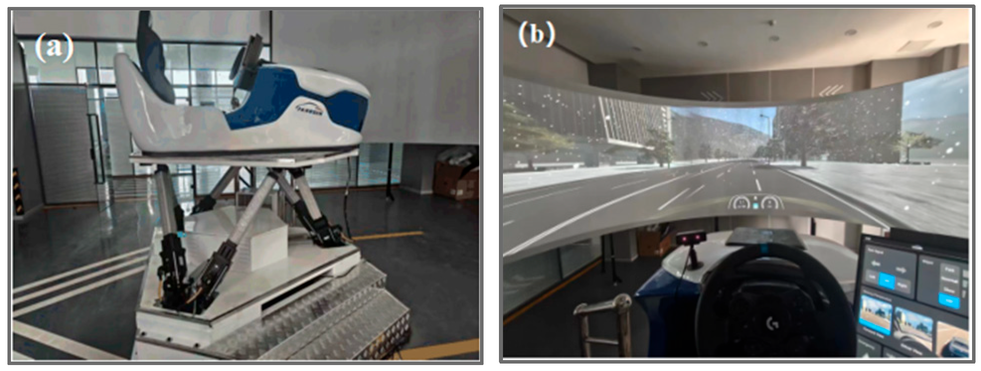
The vehicle driving simulator was composed of a visual simulation system, a control load simulation system, a sound environment simulation system, a computer data processing system, a cockpit simulation system, and a motion simulation system. The motion simulation system linked six electric cylinders through the cockpit to realize the 6-DOF motion of the body. The driving simulator was also equipped with a high-precision data acquisition system, which used a multi-sensor array to capture vehicle dynamic information in real time, including positioning coordinates, speed variables, steering angle, throttle response, and other parameters. Real-time data processing and feedback were carried out through panosim5.0 software. The traffic simulation system was composed of a circular screen with a horizontal angle of view of 180° and a vertical angle of view of 30°, as shown in Figure 1.

2.2. Participants

G-Power3.1 software was used to estimate the number of personnel needed for the experiment. The experiment was designed for a single group of repeated measurements. The parameter settings were as follows: effect size f = 0.25; alpha = 0.05; power (1—β) = 0.80; number of group s = 1; number of measurements = 4; corr among rep measures = 0.70; and nonsphericity correction ε = 1. The results showed that the minimum total sample size was 15. The final subjects of the study were 16, which met the sample size requirements.

Through the subject database, a total of 16 test drivers with normal vision or normal corrected vision were recruited to participate in the test, including 8 males and 8 females. Each driver was required to learn the operation process of the driving simulator before driving formally. In order to avoid test termination caused by improper operation of the driver, the driver was required to conduct a pretest for 1–2 min before the formal test to understand the operation methods including acceleration, braking, steering, and turning on lights.

2.3. Test Scenario Construction

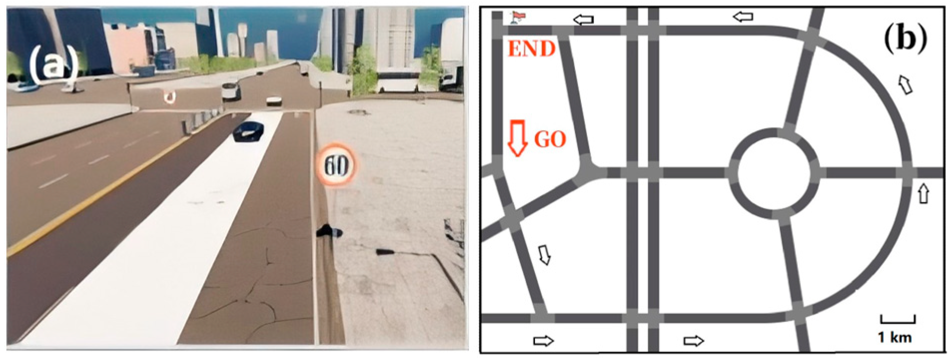
The traffic simulation scene was constructed by using PanoSim5.0 software, as shown in Figure 2a. The urban road model was a two-way three-lane model with a single lane width of 3.5 m. It had public elements in real road conditions such as buildings, road signs, trees, sidewalks, and traffic lights. The 35 km long road was mainly composed of straight roads or curved sections with visual straightening effect (with a diameter of 8000 m). A traffic light controlled intersection was set every 3 km, and the maximum speed of the whole road was limited to 60 km/h. The initial setting was that the distance between the vehicle and the vehicle to be followed was 100 m, and the vehicle to be followed would change its speed from 30 to 50 km/h in the form of an approximate sine wave at a frequency of about 0.03 Hz (which means that the vehicle to be followed reaches its minimum/maximum speed of 30/50 km/h every 33.3 s and oscillates between them). The driving route is shown by the arrow in Figure 2b, while the “GO” sign in the figure is the start position of the experiment and the “END” sign is the end position of the experiment. Four different weather conditions of sunny, rainy, snowy and foggy were set in the scene, and the driver behavior under different weather conditions was discussed.

2.4. Test Process

The experiment was carried out according to the following steps:

• The content of the experiment was introduced and the driving task on urban roads was explained in detail to the drivers until they fully understood the experimental procedure.
• The pilot entered the cockpit, familiarized themselves with the driving simulator, and conducted a 1–2 min test drive until they became accustomed to the driving operation task.
• The driver completed the specified car-following task in the simulation scene.
• After the experiment was completed, the simulated driving was stopped, the experimental data were saved, and the equipment was turned off.
• In each experiment, participants were randomly assigned to traffic scenarios they had not experienced before; additionally, they may only take part in the next experiment at least three days later.

2.5. Data Analysis

The driving behavior data, such as steering wheel angle, throttle opening, vehicle speed, acceleration, and headway, were collected by the driving simulator with the sampling frequency of 100 Hz. The steering wheel angle and acceleration were calculated in absolute values, and the average value of each index is calculated according to Formula (1).

$${\mathrm{V}}_j={\displaystyle \frac{{\displaystyle \sum _i^n\left|{\mathrm{X}}_{ij}\right|}}{n}}$$

(1)

where V_j refers to the research index, X_ij refers to the collected data of different indexes, and n refers to the number of data collected.

The impact of different weather conditions, such as the four levels of sunny, rainy, snowy, and foggy, on the driving performance index V_j was taken as an example. The original hypothesis of the test was:

$$\mathrm{H}0: \mathrm{\mu }\mathrm{b}1 = \mathrm{\mu }\mathrm{c}1 = \mathrm{\mu }\mathrm{d}1 = \mathrm{\mu }\mathrm{e}1$$

(2)

Alternative assumptions were:

$$\mathrm{H}1: \mathrm{\mu }\mathrm{b}1, \mathrm{\mu }\mathrm{c}1, \mathrm{\mu }\mathrm{d}1, \mathrm{\mu }\mathrm{e}1 \mathrm{Not} \mathrm{exactly} \mathrm{equal}$$

(3)

In Equation (1), µb1, µc1, µd1, µe1 are the mean values of V_j on sunny, rainy, snowy and foggy days, respectively. Since the test considered the sampling of the same driver in different weather environments, and the number of environmental variables was greater than 2, the repeated measurement analysis of variance was used for analysis. Different weather environments were used as intra group variables for test analysis. During the data test, the significance level was set to 0.05. When p < 0.05, the original hypothesis was rejected and the alternative hypothesis was selected.

2.6. Setting of Simulated Traffic Environments

The experimental parameters were set according to different weather conditions, such as sunny days, foggy days, rainy days, snowy days, etc. The corresponding parameter settings of the driving simulator are shown in

Table 1. Weather configuration parameters in simulator.

Weather Condition	1 h Rainfall Depth/mm	12 h Snowfall Depth/mm	Visibility/m	Friction Coefficient
Sunny	\	\	10,000	0.85
Foggy	\	\	80	0.85
Rainy	10 mm	\	500	0.51
Snowy	\	3 mm	300	0.34

.

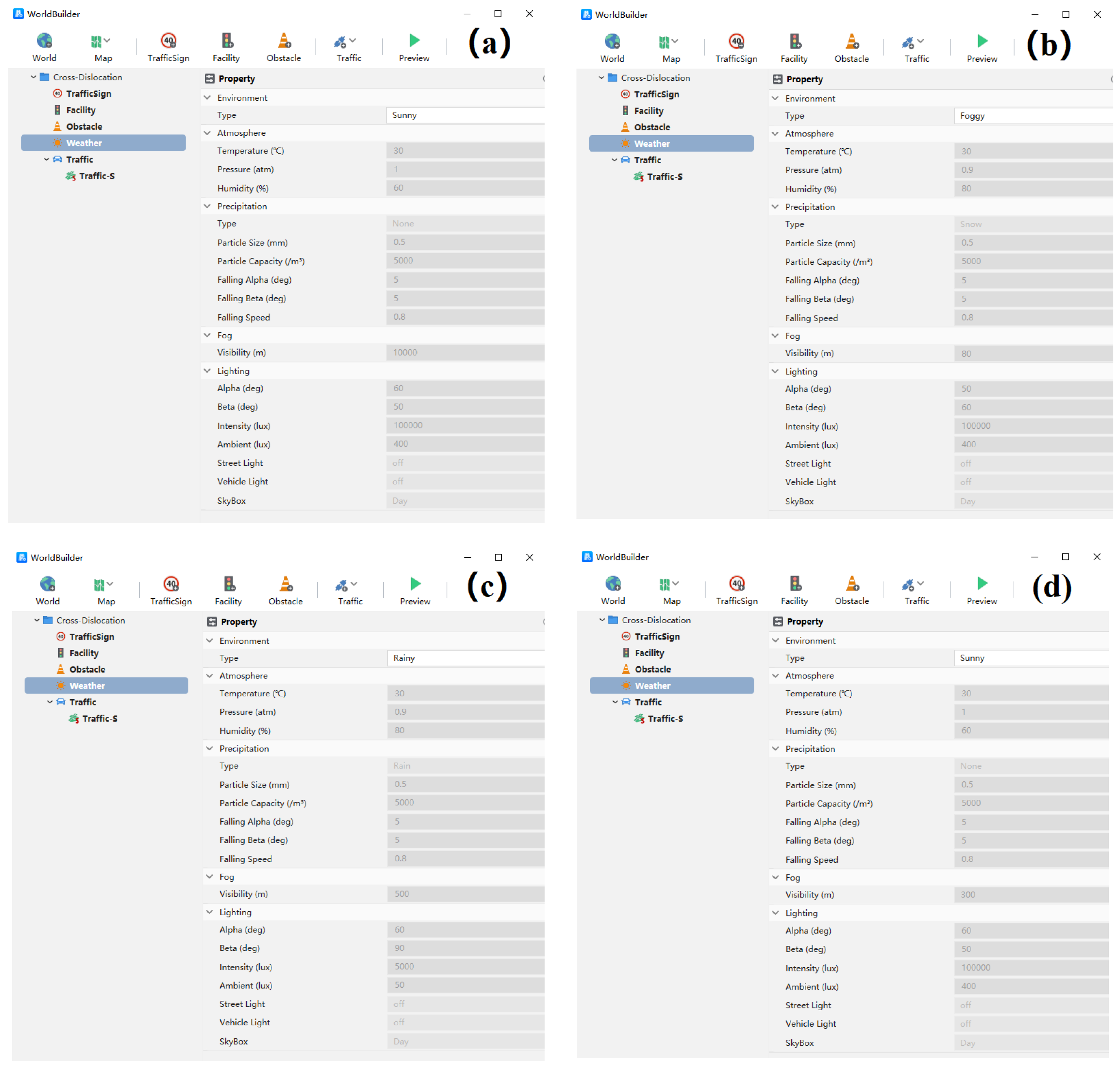
The effect of different weather conditions on the sight distance in the virtual traffic environment used a visual effect that gradually blurred from near to far. The weather parameter settings of the simulation traffic scene experiment are shown in Figure 3. Taking steering wheel angle, throttle opening, vehicle speed, acceleration, and headway as measurement indexes, the influence of weather conditions on the driver’s lateral control, longitudinal control, and car-following safety was analyzed.

3. Results and Discussion

In order to evaluate the robustness of the sample size under more conservative conditions, a sensitivity analysis of corr among rep measures and nonsphericity correction ε coefficient were carried out. The results of the analysis are shown in

Table 2. Estimation of sample size based on g_power.

Corr Among Rep Measures	Nonsphericity Correction ε	Sample Size
0.7	1	15
0.7	0.9	16
0.7	0.8	17
0.6	0.8	20
0.6	0.7	21

.

Considering the difficulty of the experiment, 16 subjects were recruited in this study. In order to evaluate the sufficiency of sample size, a sensitivity analysis was carried out. When corr = 0.60 and ε = 0.70, the required sample size was increased to 21 people. This indicated that, under strict conditions, the current sample size may be slightly insufficient. However, with the exception of throttle opening, the effect sizes for the other key indicators were relatively large and remained statistically significant after Greenhouse–Geisser correction (p < 0.05). This suggests that, despite the relatively small sample size, the observed effect sizes were sufficient to support the reliability of the study’s conclusions.

3.1. Steering Wheel Angle

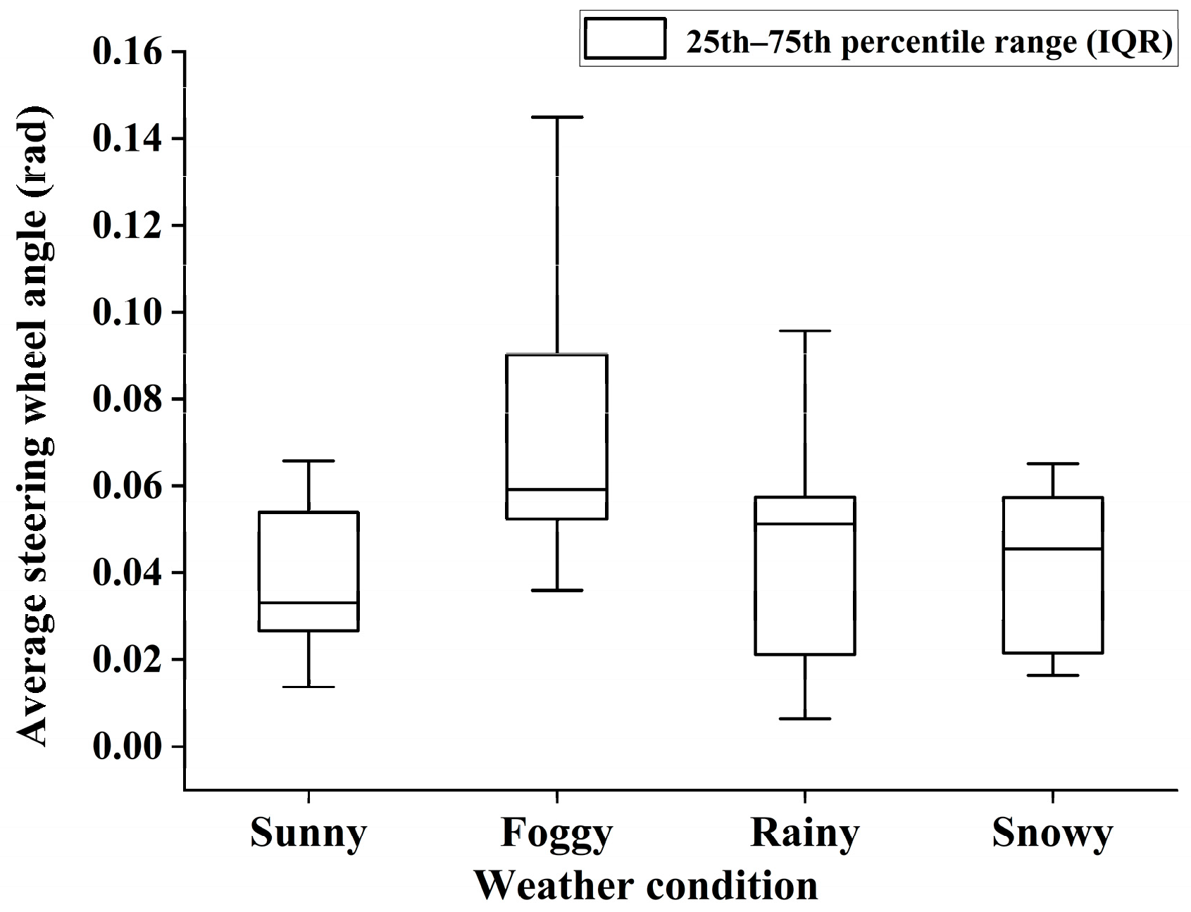
The steering wheel angle, as an important index of vehicle lateral handling performance, is usually used to characterize the accuracy of driver steering operation. The larger the steering wheel angle, the worse the lateral stability of the vehicle, and the easier it is to cause traffic accidents. Since the turning road has certain interference with the analysis of the reverse wheel angle, the study only analyzed the straight highway sections. Mauchly’s sphericity test results showed that W = 0.512, p = 0.102 > 0.05, ε_GG = 0.721, ε_HF = 0.795. Therefore, by assuming sphericity analysis, F(3, 45) = 7.054, p = 0.001, η_p² = 0.320. Since ε_GG was less than 0.75, combined with the analysis of Greenhouse–Geisser, the corrected results showed that (F(2.034, 30.508) = 7.05, p = 0.003, η_p² = 0.320) the p values of both were less than 0.05. This showed that the change in weather conditions on straight kilometers had a significant impact on the steering wheel angle. Bonferroni post hoc tests showed that there were significant differences between sunny and snowy days (p = 0.016 < 0.05), as well as foggy days and snowy days (p = 0.021 < 0.05).

As shown in Figure 4, the average steering wheel angle in a single weather environment was sunny day: 0.039 rad; fog: 0.073 rad; rainy day: 0.046 rad; and snow: 0.042 rad. This was similar to the conclusion of Saffarian et al. in their study of risk perceptions and lateral control in the process of automatic and manual car following in fog [14]. This showed that when the weather environment became worse, the driver’s line of sight was blocked, which affected the capture of traffic information and required more active lateral control behavior to obtain more traffic information. It can be seen from Figure 3 that the average steering wheel angle was the highest on foggy days, the lowest on sunny days, and the difference was small on rainy and snowy days, further indicating that the line of sight was most severely blocked on foggy days and the driver had to obtain more traffic information through lateral control.

3.2. Headway

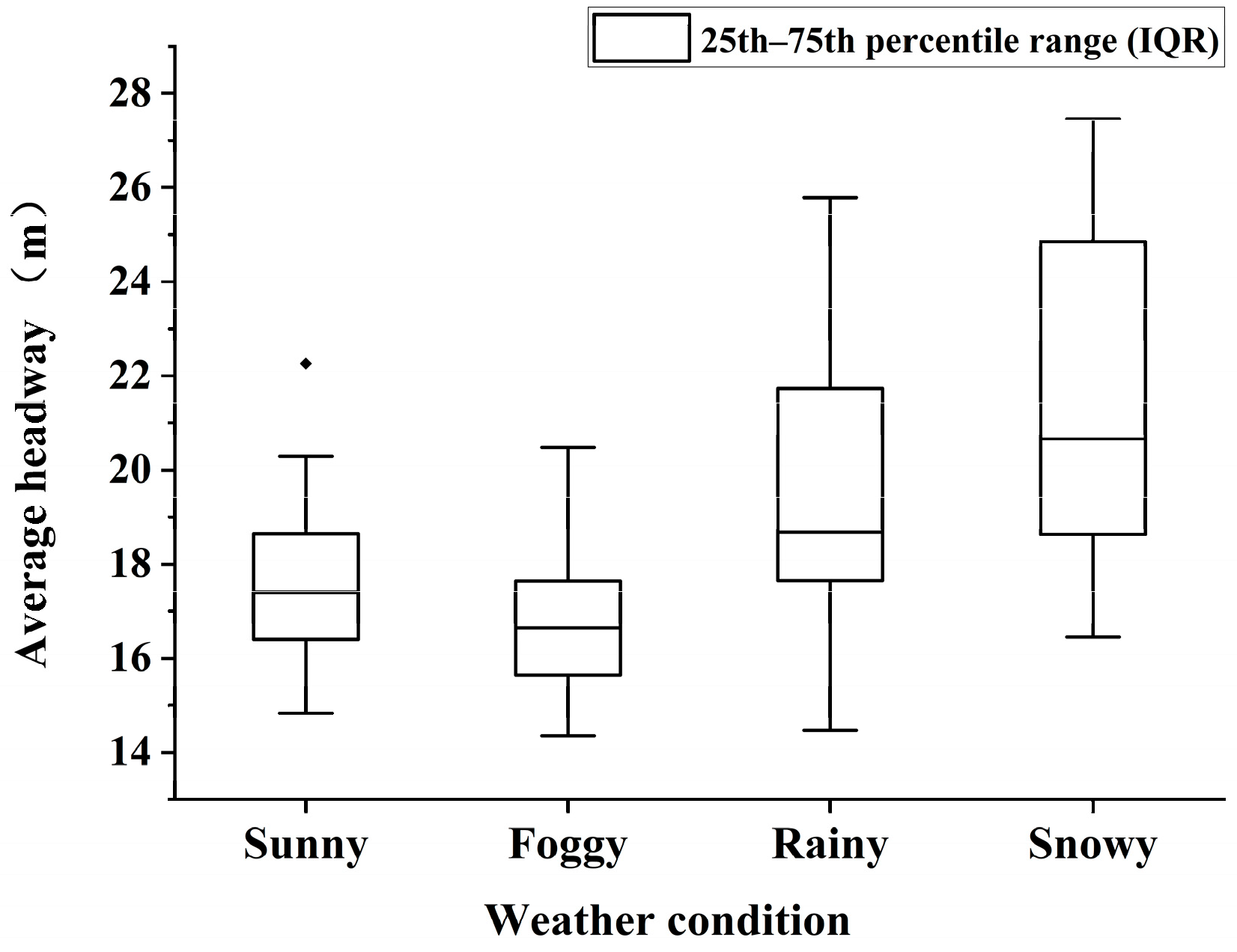
In urban roads, excessive headway will affect the driving speed of their own vehicles and the vehicles behind them, which will then affect the traffic. If the headway is too small, the driving safety is directly reduced. After the normality test, the data followed the normal distribution. Mauchly’s sphericity test results showed that W = 0.547, p = 0.142 > 0.05, ε_GG = 0.781, ε_HF = 0.935. According to the assumed sphericity analysis, F(3, 45) = 8.412, p = 0.001, η_p² = 0.359. Since ε_GG wass less than 0.9, combined with Huynh–Feldt analysis, the corrected results showed that (F(2.806, 42.089) = 8.412, p = 0.001, η_p² = 0.320) the p values were less than 0.05. The results showed that the change in weather conditions had a significant impact on the headway. Bonferroni post hoc tests showed that there were significant differences between sunny and snowy days (p = 0.015 < 0.05), as well as between foggy and snowy days (p = 0.005 < 0.05). As shown in Figure 5, the average headway in a single weather environment was sunny day: 17.759 m; foggy day: 16.759 m; rainy day: 19.812 m; and snowy day: 21.275 m. The research results showed that the driver would shorten the following distance at lower speeds in the traffic environment with blocked vision on foggy days [15].

However, while the headway between snowy and rainy days was significantly longer, which was consistent with the research of Rahma et al. on rainy and snowy days, the friction coefficient of the road surface was reduced, the braking distance was longer, and the driver could prevent a rear-end collision through a longer headway [16].

3.3. Throttle Opening

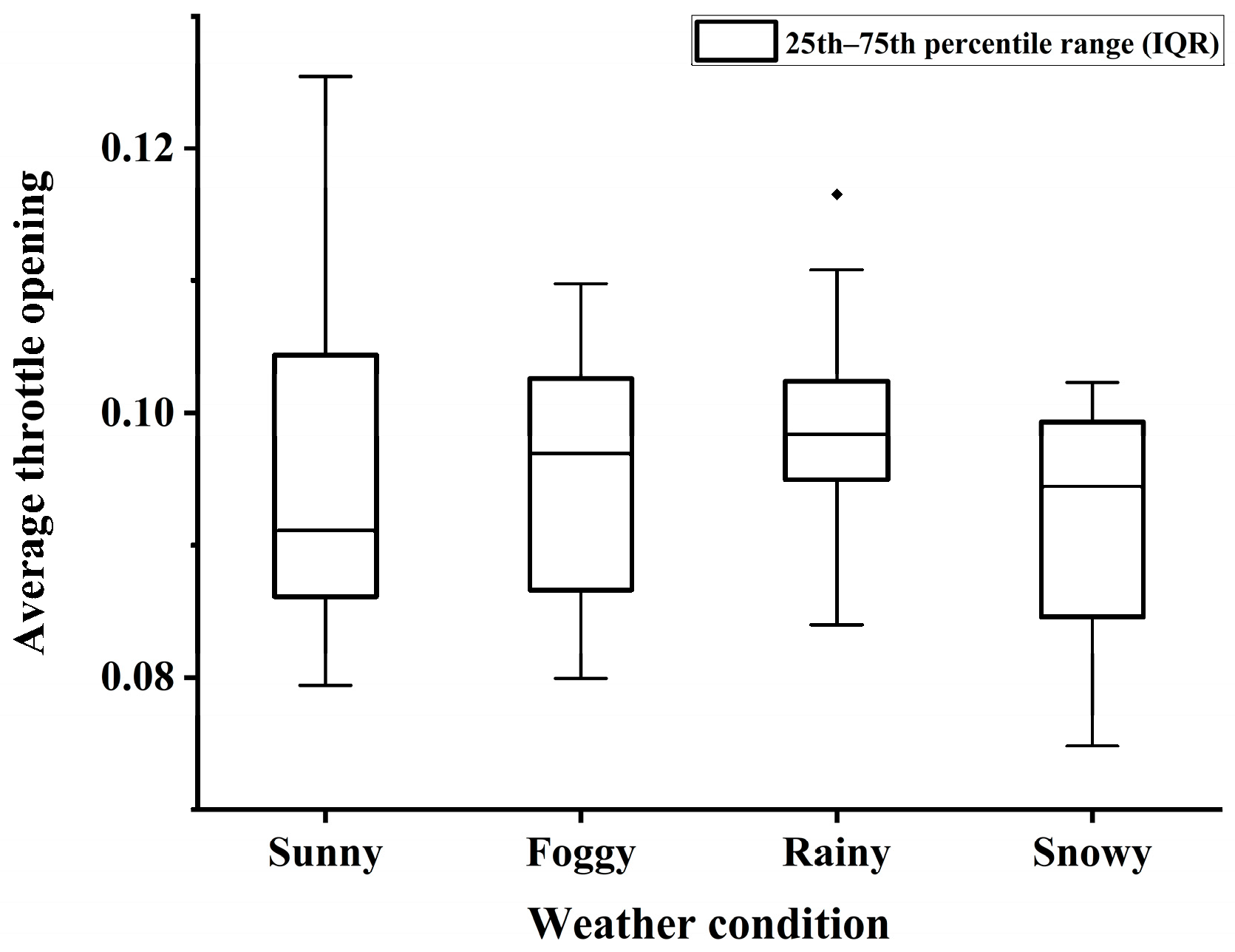
The throttle opening is used to indicate the driver’s control of the vehicle’s accelerator pedal. After the normality test, the data obeyed the normal distribution. Mauchly’s sphericity test results showed that W = 0.721, p = 0.482 > 0.05, ε_GG = 0.820, ε_HF = 0.993. As this was consistent with the spherical test results, the assumed sphericity analysis was accordingly F(3, 45) = 1.246, p = 0.304, η_p² = 0.077. Since ε_GG was less than 0.9, combined with Huynh–Feldt analysis, the corrected results showed that (F(2.979, 44.689) = 1.246, p = 0.304, η_p² = 0.077) the p values were greater than 0.05. The results showed that the change in weather conditions had a significant impact on the throttle opening. As shown in Figure 6, the average throttle opening in a single weather environment was sunny day: 0.103; foggy day: 0.105; rainy day: 0.108; and snowy day: 0.0980 The throttle opening was around 0.100 in all four weather condition types, and the difference was not obvious. This may be because the throttle opening was directly related to the vehicle speed. In any weather, the vehicle speed was not different from the vehicle speed in front, so the average throttle opening was close.

3.4. Vehicle Speed Standard Deviation and Acceleration

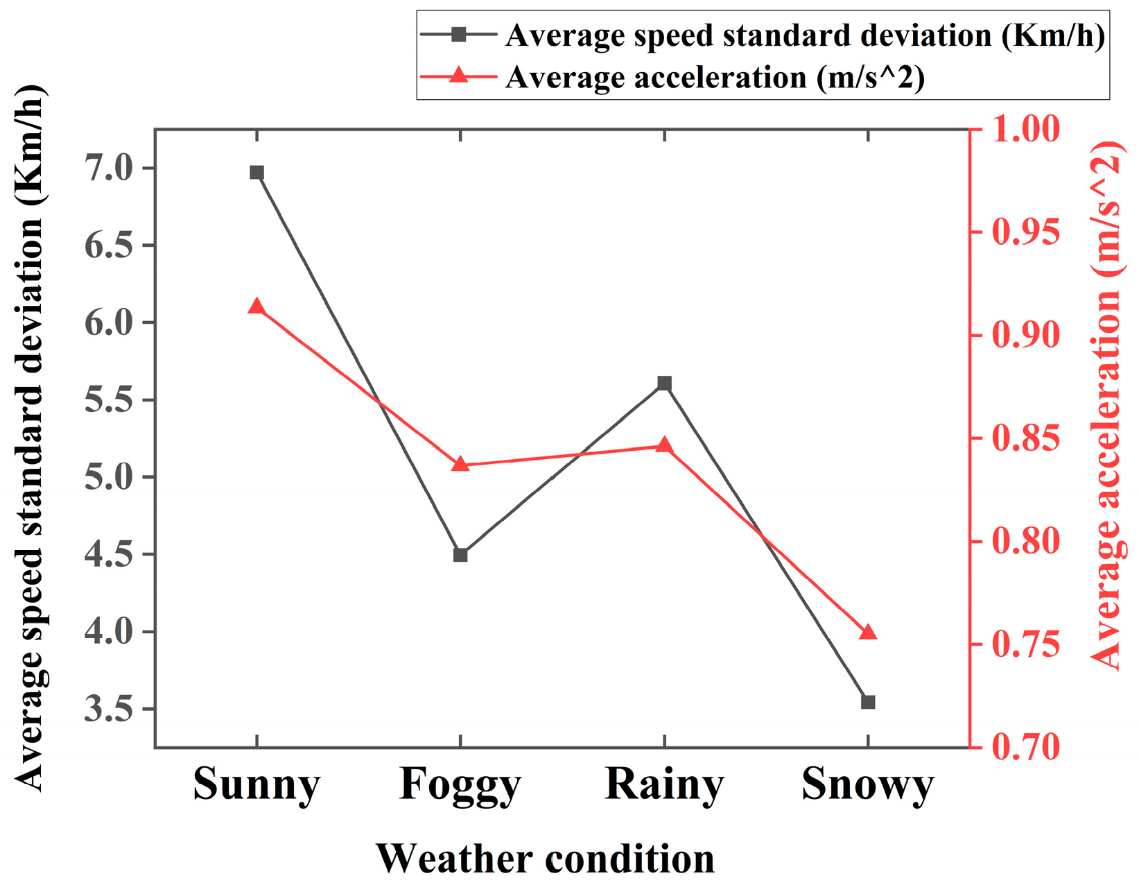
When the speed of the following vehicle is constant, the closer the vehicle speed is to the following vehicle, and the better the following effect is; conversely, the greater the standard deviation of vehicle speed, the greater the fluctuation of vehicle speed, and the greater the risk during driving. In this study, the standard deviation of speed represented the standard deviation of the relative velocity (Δv) between the lead vehicle and the following vehicle. After the normality test, the data followed the normal distribution. Mauchly’s sphericity test results showed that W = 0.707, p = 0.447 > 0.05, ε_GG = 0.801, ε_HF = 0.964. As this was consistent with the spherical test results, the assumed sphericity analysis was F(3, 45) = 186.3561, p = 0.001, η_p² = 0.926. Because ε_GG was less than 0.9, combined with Huynh–Feldt analysis, the corrected results showed that (F(2.893, 43.390) = 186.356, p = 0.001, η_p² = 0.926) the p values were less than 0.05. The results showed that the change in weather conditions has a significant impact on the standard deviation of vehicle speed. Bonferroni post hoc tests showed significant differences between sunny and foggy days (p = 0.001 < 0.05); sunny and rainy days (p = 0.001 < 0.05); sunny and snowy days (p = 0.001 < 0.05); foggy and rainy days (p = 0.001 < 0.05); foggy and snowy days (p = 0.001 < 0.05); and rainy and snowy days (p = 0.001 < 0.05). As shown in Figure 7, the standard deviation of vehicle speed dropped significantly with the occurrence of harsh weather environments (sunny day: 6.971 km/h; fog: 4.496 km/h; rainy day: 5.607 km/h; and snow: 3.544 km/h). The results indicated that the driving speeds in urban car-following scenarios were susceptible to weather variations. As the traffic environment deteriorated, speed fluctuations diminished, leading to more stable driving behavior.

Acceleration can be used to indicate the driver’s control over vehicle acceleration and deceleration, reflecting the stability of vehicle longitudinal handling. After the normality test, the data followed the normal distribution. Mauchly’s sphericity test results showed that W = 0.768, p = 0.607 > 0.05, ε_GG = 0.851, ε_HF = 0.1. As this was consistent with the spherical test results, the assumed sphericity analysis was F(3, 45) = 10.010, p = 0.001, η_p² = 0.400. Because ε_GG was less than 0.9, combined with Huynh–Feldt analysis, the corrected results showed that the p values (F(3, 35) = 10.010, p = 0.001, η_p² = 0.400) were less than 0.05, indicating that the change in weather conditions had a significant impact on the acceleration. Bonferroni post hoc tests showed significant differences between sunny and rainy days (p = 0.048 < 0.05); sunny and snowy days (p = 0.001 < 0.05); and foggy and snowy days (p = 0.031 < 0.05). As shown in Figure 7, the acceleration varied under different weather conditions (sunny day: 0.913 m/s²; fog: 0.837 m/s²; rainy day: 0.846 m/s²; and snow: 0.755 m/s²). In addition, it can be seen from the figure that the trend in velocity standard deviation and acceleration was relatively consistent. As shown in Figure 6, the acceleration decreased with the introduction of abnormal weather factors, and the acceleration in snowy weather was the smallest, which was consistent with the results of Ahmed et al. in their study of the impact of rain on headway [3].

3.5. Number of Collisions

Collision frequency can be used to characterize vehicle safety under different weather conditions. However, there was a significant difference between novice drivers and experienced drivers in the number of dangerous driving incidents. In accordance with previous studies, drivers with a driving mileage exceeding 30,000 km were defined as experienced drivers, while those with a mileage below 30,000 km were classified as novice drivers. The study included seven novice drivers and nine experienced drivers. The driver collision data are presented in

Table 3. Number of collisions per participant under different weather conditions.

Participant	Mileage (10,000 km)	Number of Collisions
		Sunny	Foggy	Rainy	Snowy
1	>5	0	0	0	0
2	>3	0	1	0	0
3	>5	0	0	0	1
4	<1	0	1	1	0
5	>3	0	1	0	0
6	<1	0	0	1	1
7	>1	1	1	0	0
8	>3	0	0	0	0
9	<1	2	1	1	2
10	>5	0	0	0	0
11	>1	0	0	0	1
12	>3	0	0	0	0
13	<1	1	2	0	1
14	<1	1	1	0	0
15	>3	0	0	1	1
16	>3	0	0	0	0

.

Since the number of collisions was a discrete variable, a regression model was employed for analysis. The Pearson’s χ²/df = 0.79, which was less than 1, indicated no evidence of overdispersion in the data. However, given that the quasi-likelihood under the independence model criterion (QIC) for the negative binomial regression (QIC = 36.09) was lower than that of the Poisson regression (QIC = 48.12), the negative binomial regression model was selected for further analysis. The test results are presented in

Table 4. Effect test of negative binomial model before data optimization.

Variable	Wald Chi-Square	df	Sig.
Weather	5.527	3	0.137
Mileage	11.711	1	0.001

. As shown in Table 3, the p-value for weather conditions was 0.137, which was greater than 0.05, indicating that weather did not have a statistically significant effect on the frequency of collisions. In contrast, the p-value for driving experience was 0.001, which was less than 0.05, demonstrating that driving experience had a significant impact on the number of collisions.

The test results revealed that two novice drivers were involved in a relatively high number of traffic accidents during the experiment: Driver 9 was involved in six accidents, while Driver 13 was involved in four accidents. After excluding these two drivers, negative binomial regression analysis was performed again, and the results are presented in Table 4. As shown in

Table 5. Effect test of negative binomial model after data optimization.

Variable	Wald Chi-Square	df	Sig.
Weather	4.321	3	0.229
Mileage	8.119	1	0.004

, the p-value for different weather conditions was 0.229 (>0.05), and the p-value for driving experience was 0.004 (<0.05). The analysis results after exclusion were consistent with those before exclusion, indicating that driving experience was a key factor affecting collision frequency, whereas weather conditions showed no significant effect in this experiment.

4. Conclusions

(1)

Through the analysis of steering wheel angles, it can be seen that in bad weather, when the driver’s line of sight is blocked, it will strengthen the trimming of steering wheel angle, resulting in poor vehicle lateral stability.

(2)

When following a car on an urban road, the variation trends in the standard deviation of vehicle speed and acceleration are relatively consistent under different weather conditions. In bad weather, the fluctuation of the standard deviation of vehicle speed and acceleration decreases based on the safety of the driver.

(3)

The headway is the smallest on foggy days, followed by sunny and rainy days, and the largest on snowy days. This is because the traffic vision is poor on foggy days, and the purpose of following the car is achieved by reducing the headway. On rainy and snowy days, the friction coefficient between the ground and the tire becomes smaller, resulting in a larger headway.

(4)

Under different weather conditions, the number of collisions does not show significant differences. However, when drivers are divided into novice drivers and experienced drivers, they show significant differences in the number of collisions. Novice drivers have a higher probability of traffic accidents while driving.

References

1. Kircher, K.; Ahlström, C. Attentional Requirements on Cyclists and Drivers in Urban Intersections. Transp. Res. Part F Traffic Psychol. Behav. 2020, 68, 105–117. [Google Scholar] [CrossRef]
2. Helbing, D.; Tilch, B. Generalized force model of traffic dynamics. Phys. Rev. E 1998, 58, 133–138. [Google Scholar] [CrossRef]
3. Ahmed, M.M.; Ghasemzadeh, A. The Impacts of Heavy Rain on Speed and Headway Behaviors: An Investigation Using the Shrp2 Naturalistic Driving Study Data. Transp. Res. Part C Emerg. Technol. 2018, 91, 371–384. [Google Scholar] [CrossRef]
4. Wu, Y.; Abdel-Aty, M.; Cai, Q.; Lee, J.; Park, J. Developing an algorithm to assess the rear-end collision risk under fog conditions using real-time data. Transp. Res. Part C Emerg. Technol. 2018, 87, 11–25. [Google Scholar]
5. Ma, M.; Ma, G.; Liang, S. Density waves in car-following model for autonomous vehicles with backward looking effect. Appl. Math. Model. 2021, 6, 1–12. [Google Scholar] [CrossRef]
6. Huang, Y.X.; Rui, J.; Zhang, H.M.; Hu, M.B.; Tian, J.F.; Jia, B.; Gao, Z.Y. Experimental study and modeling of car-following behavior under high speed situation. Transp. Res. 2018, 97, 194–215. [Google Scholar] [CrossRef]
7. Bella, F.; Russo, R. collision warning system for rear-end collision: A driving simulator study. Procedia-Soc. Behav. Sci. 2011, 20, 676–686. [Google Scholar] [CrossRef]
8. Broughton, K.L.M.; Switzer, F.; Scott, D. Car following decisions under three visibility conditions and two speeds tested with a driving simulator. Accid. Anal. Prev. 2007, 39, 106–116. [Google Scholar] [CrossRef] [PubMed]
9. Hammit, B.E.; Ghasemzadeh, A.; James, R.M.; Ahmed, M.M.; Young, R.K. Evaluation of weather-related freeway car-following behavior using the SHRP2 naturalistic driving study database. Transp. Res. Part F Traffic Psychol. Behav. 2018, 59, 244–259. [Google Scholar] [CrossRef]
10. Cassidy, M.J.; Windover, J.R. Drive memory: Motorist selection and retention of individualized headways in highway traffic. Transp. Res. Part F 1998, 6, 129–137. [Google Scholar]
11. Chen, C.; Zhao, X.; Liu, H.; Ren, G.; Liu, X. Influence of adverse weather on drivers’ perceived risk during car following based on driving simulations. J. Mod. Transp. 2019, 27, 282–292. [Google Scholar] [CrossRef]
12. Gong, B.; Wei, R.; Wu, D.; Lin, C. Fleet management for HDVs and CAVs on highway in dense fog environment. J. Adv. Transp. 2020, 2020, 8842730. [Google Scholar] [CrossRef]
13. Kang, J.J.; Ni, R.; Andersen, G.J. The effects of reduced visibility from fog on car following performance transportation research record. Transp. Res. Rec. J. Transp. Res. Board 2008, 2069, 9–15. [Google Scholar] [CrossRef]
14. Saffarian, M.; Happee, R.; Winter, J.C.F.D. Why do drivers maintain short headways in fog? A driving-simulator study evaluating feeling of risk and lateral control during automated and manual car following. Ergonomics 2012, 55, 971–985. [Google Scholar] [CrossRef] [PubMed]
15. Ni, R.; Kang, J.J.; Andersen, G.J. Age-related declines in car following performance under simulated fog conditions. Accid. Anal. Prev. 2010, 42, 818–826. [Google Scholar] [CrossRef] [PubMed]
16. Rahman, A.; Lownes, N.E. Analysis of rainfall impacts on platooned vehicle spacing and speed. Transp. Res. Part F Traffic Psychol. Behav. 2012, 15, 395–403. [Google Scholar] [CrossRef]
Figure 1. Test equipment: (a) driving simulator; (b) screen of driving simulator.
Vehicles 08 00056 g001
Figure 2. Traffic scenario design: (a) simulated driving scenario; (b) simulated driving route.
Vehicles 08 00056 g002
Figure 3. Weather parameter setting in panosim software: (a) sunny; (b) foggy; (c) rainy; and (d) snowy.
Vehicles 08 00056 g003
Figure 4. Steering wheel angle under different weather conditions.
Vehicles 08 00056 g004
Figure 5. Headway under different weather conditions.
Vehicles 08 00056 g005
Figure 6. Throttle opening under different weather conditions.
Vehicles 08 00056 g006
Figure 7. Standard deviation of speed and acceleration under different weather conditions.
Vehicles 08 00056 g007