Collaborative Control of Rear-Wheel Independent Drive Electric Vehicles During Tire Blowouts Using Broad-Extreme Reinforcement Learning: Simulation and Scaled Prototype Verification

Abstract

Tire blowouts represent one of the most hazardous fault scenarios for electric vehicles (EVs). While collaborative active steering control (ASC) and direct yaw moment control (DYC) can theoretically maintain stability during these events, the strong coupling effects between them make controller design challenging. To address this, an adaptive control algorithm based on broad-extreme reinforcement learning (RL), named broad critic extreme actor (BCEA), is proposed. Compared to traditional controllers, the proposed BCEA architecture is simpler to design and demonstrates enhanced robustness. Crucially, it achieves significantly faster training speed than traditional RL methods such as deep deterministic policy gradient (DDPG). Both simulation and scaled prototype tests verify the ability of the BCEA-based controller to maintain vehicle stability during different types of tire blowout scenarios. Furthermore, compared to traditional RL methods, the training efficiency is improved by more than 80%. These results indicate that the proposed BCEA controller is a promising advancement for vehicle stability control under critical failure conditions.

1. Introduction

Electric vehicles (EVs) represent a promising solution to current emission challenges [1]. However, like conventional internal combustion engine vehicles (ICEVs), EVs remain susceptible to tire blowouts. These blowouts are critical safety hazards that can cause severe path deviation, increased energy consumption and serious accidents [2]. The mechanical limitations of ICEVs prevent the real-time adjustment of driving forces required to maintain stability during such failures. In contrast, EVs can be controlled precisely, with the ability to rapidly adjust output torque to stabilize the vehicle immediately with tire blowouts. Furthermore, independent drive EVs (IDEVs) offer superior force distribution compared to conventional configurations. Among these, rear-wheel independent drive EVs (RWID EVs) feature a simpler mechanical design, optimized driving dynamics, reduced unsprung mass and enhanced directional stability compared to four-wheel independent drive EVs [3,4]. Moreover, while four-wheel systems provide comprehensive stability control, the RWID configuration offers an advantageous balance between performance and mechanical simplicity. Therefore, developing effective controllers for RWID EVs under tire blowout conditions represent a highly promising research direction. These controllers could significantly enhance the safety and reliability of EV operations, further strengthening their viability as a sustainable transportation solution.

Currently, active steering control (ASC) and direct yaw moment control (DYC) are two extensively employed methods for addressing EV stability issues induced by tire blowouts. ASC is widely recognized as an effective approach for maintaining stability, because it functions by adjusting front wheel steering angles to counteract the lateral force generated by a tire blowout. Several classic control strategies are applied to ASC. Proportional–integral–derivative (PID) control [5] and linear quadratic regulator (LQR) [6,7,8] are frequently used, with PID enabling rapid steering response and LQR ensuring high control precision. Additionally, strategies such as fuzzy control [9,10], adaptive control [11,12], and sliding mode control (SMC) [13,14,15] are also commonly applied to ASC. These methods excel at adapting to the nonlinear dynamic characteristics of EVs following a tire blowout, allowing the vehicle to precisely track its ideal trajectory. Apart from ASC, DYC is another method for stabilizing EVs during tire blowouts. The core operation of DYC involves two sequential parts. First, it calculates the desired yaw moment required for stability. Second it distributes torque to each driving wheel based on this target moment. DYC strategies are generally divided into two categories. The first includes traditional algorithms, including PID control [16], LQR [17,18,19], model predictive control (MPC) [20,21], and SMC [22,23]. The second category consists of intelligent algorithms, such as fuzzy control [24,25] and neural network control [26,27,28], which are particularly effective in handling the complex uncertainties of tire blowout scenarios. In summary, both ASC and DYC represent primary and reliable strategies for EV stability during tire blowouts.

However, practical applications of vehicle stability still face numerous challenges during emergency situations. First, conventional algorithms rely heavily on vehicle models. Tire blowout scenarios exhibit complex nonlinear dynamics that can cause a sudden decline in the performance of model-dependent controllers. Developing accurate models for these scenarios remain difficult, as simulations often oversimplify critical factors like dynamic tire behavior, resulting in significant deviations from real-world conditions. Second, traditional control algorithms struggle with parameter tuning. Parameters that are effective under specific conditions often prove inadequate when vehicle speeds or road conditions change, potentially degenerating vehicle stability. Third, standalone control systems, using either ASC or DYC in isolation, have fundamental structural limitations. Neither system alone can effectively control the vehicle during a tire blowout. ASC is mechanically constrained and often cannot provide adequate steering correction force. Similarly, the effectiveness of DYC is reduced when tire blowouts lead to sudden drops in cornering stiffness, disrupting the force and moment equilibrium of the vehicle. These combined challenges of model dependency, parameter sensitivity, and structural limitations imply the necessity of an integrated approach. Consequently, developing a control system that integrates both ASC and DYC represents a critical step towards enhancing vehicle stability during tire blowout emergencies.

Currently, collaborative ASC and DYC for electric vehicles are widely used. These methods are often developed through several approaches, including cost-based coordination [29], multi-level cooperation [30], optimized sliding mode control [31], and model predictive control [32]. Collaborative ASC and DYC are also applied to fault-tolerant control in vehicles [33,34,35,36]. These studies show that collaborative ASC and DYC are effective for both stability control and fault-tolerant control. However, existing methods still face significant challenges. They often rely on vehicle models that are difficult to establish accurately, especially when the tire blowout is considered. Additionally, these methods require complex real-time weight adjustments to adapt to nonlinear systems. Moreover, these methods suffer from high computational complexity, and this complexity hinders rapid response. Therefore, existing collaborative ASC and DYC cannot be directly used for vehicle stability control under tire blowing out conditions.

To overcome the above problems of the collaborative ASC and DYC, new methods should be proposed and introduced. The application of rapidly involving artificial intelligence (AI) technologies to vehicle control has emerged as a highly promising solution. Among various AI techniques, reinforcement learning (RL) offers unique advantages for handling complex scenarios including tire blowouts. Unlike traditional controllers, RL does not rely on complex physical vehicle models. Instead, it enables agents to construct adaptive controllers directly through interactions, thereby eliminating the need for manual parameter tuning. Building on these advantages, this research demonstrates how RL can effectively integrate ASC and DYC. The optimal weight distribution between ASC and DYC is automatically determined by an RL agent without manual intervention. Moreover, the RL-based controller adapts dynamically to varied driving conditions and specific tire blowout locations. Despite a blowout occurring at the front or rear axle, the RL-based controllers are capable of instantly recalibrating its control strategy to maintain vehicle stability. Consequently, RL represents a robust approach for achieving precise and efficient vehicle control during tire blowout scenarios. This significantly enhances vehicle safety by providing context-sensitive responses that potentially reduce accident rates.

Traditional RL algorithms often exhibit significant limitations when used in tire blowout control problems. For instance, Q-learning [37,38] requires discretization of state spaces, which proves impractical for the complex dynamics inherent in tire blowout scenarios. Deep Q network (DQN) [39,40] improves state representation using neural networks, yet it still suffers from the limitation of discrete action outputs, which restrict its applicability for precise vehicle control. Furthermore, deep deterministic policy gradient (DDPG) [41,42] addresses the discretization problem but requires the training of multiple neural networks, resulting in substantially reduced training efficiency. Many RL-based studies have been conducted for collaborative ASC and DYC. Twin delayed deep deterministic policy gradient (TD3) [43,44] and proximal policy optimization (PPO) are RL-based methods which are often used as controllers [45,46]. These methods are also applied to ASC and DYC [47,48,49,50]. However, these methods have fundamental limitations. PPO relies on a complex value model design, which increases training complexity. Additionally, TD3 requires high computational resources, which leads to slow training speeds. TD3 is also highly sensitive to hyperparameters that require extensive fine-tuning. Therefore, using reinforcement learning alone for collaborative ASC and DYC is insufficient to overcome the limitations of current methods for collaborative ASC and DYC.

To overcome the above limitations, a broad critic deep actor (BCDA) algorithm is developed [51], which enhances the DDPG architecture by replacing the critic network component with a broad learning system (BLS) [52]. As demonstrated in [51], this innovation significantly improves training efficiency while maintaining precision control. Moreover, our previous work successfully implemented this algorithm in several truck control scenarios [53]. These implementations highlight the potential of BCDA as a viable solution for addressing the limitations of traditional RL algorithms in vehicle stability control during tire blowouts.

Despite its high potential, the BCDA algorithm requires further optimization to ensure vehicle safety during critical failure scenarios. While the BLS-based critic in the BCDA algorithm significantly accelerates training efficiency, our preliminary analysis indicates that it induces instability during catastrophic events, such as tire blowouts. Specifically, inherent limitations in BLS node configuration [54] cause the critic to generate extreme or abnormal value estimates when encountering these outlier states. These anomalies propagate to the deep actor, which is based on a deep neural network, resulting in ill-conditioned policy gradients. This scenario often manifests as exploding or vanishing updates in the deep actor that degenerate vehicle control performance. Thus, re-evaluating BLS node selection parameters is essential to prevent these cascading failures.

To overcome the limitations of gradient descent, specifically the risk of exploding gradients and slow convergence in complex environments, a meta-hierarchy algorithm is proposed. Instead of relying on gradient-based backpropagation, this framework adopts cuckoo search (CS) for network optimization. Compared with other derivative-free meta-heuristic methods like genetic algorithms [55], CS is selected for its superior flexibility and lower computational cost in high-dimensional spaces [56,57]. To further address the computational efficiency, the deep actor network in the BCDA algorithm is replaced by an extreme learning machine (ELM) because ELM allows the system to increase the training speed [58]. The proposed training protocol operates in two stages. First, the BLS critic calculates Q-values and updates weights via pseudoinverse. Second, for a given state, the CS algorithm identifies the optimal action that maximizes the Q-value. The ELM-based actor is then analytically updated to map the state to this optimal action. This approach can eliminate gradient dependencies entirely and achieve rapid convergence while maximizing Q-value stability.

This study aims to enhance stability control of EVs during tire blowout scenario through a novel broad critic extreme actor (BCEA)-based RL approach. Existing collaborative ASC and DYC mainly rely on conventional control algorithms. However, active steering and yaw moment control show significant coupling effect in vehicle dynamics. Conventional strategies require manual decoupling and sensitivity-based control weight allocation. This process is computationally complex, likely to have design errors, and further limited by the highly nonlinear and strongly perturbed characteristics of the vehicle model under extreme conditions such as tire blowouts. Consequently, the adaptability and the robustness of traditional methods are limited. In contrast, the proposed BCEA method has good adaptability. Using neural network-based training mechanisms, control decoupling and weight allocation are automatically achieved without manual intervention. This approach greatly improves the environmental adaptability and control robustness of the system under complex and emergency conditions (such as tire blowouts). The overall performance is believed to be superior to that of traditional control strategies.

Compared with other RL methods, the proposed BCEA algorithm replaces gradient descent-based optimization strategies with CS method. This change effectively improves global optimization capability. At the same time, the ELM is also utilized. As a result, computational efficiency, convergence speed and stability of the algorithm can be improved.

By using physical experiments with a custom-developed prototype and computer simulations using a data-driven numerical framework, the effectiveness of the proposed controller is verified. The core innovations and contributions of this study are as follows:

(1)

This study proposes a new RL-based collaborative ASC and DYC controller based on BCEA that addresses the challenges related to structural complexity and low computational efficiency in traditional RL and BCDA approaches for vehicle control. Compared to existing collaborative ASC and DYC controllers, the proposed BCEA reduces system complexity and computational cost while enhancing the stability of algorithm convergence.

(2)

This study proposes a method that directly integrates tire blowout detection signals into the input layer, effectively addressing stability control challenges for electric vehicles during tire blowout events. Compared to traditional control strategies, the proposed approach enhances the system robustness and trajectory tracking accuracy in such emergency scenarios.

(3)

This study proposes road tests utilizing prototype vehicles, mitigating safety risks associated with real vehicle tests under tire blowout conditions. Compared to traditional testing methods, the proposed approach enhances scenario diversity and test repeatability while eliminating potential safety hazards.

The remainder of this paper is structured as follows. Section 2 reviews vehicle tire fault diagnosis methods. Section 3 details the architecture, working principle and training protocol of the BCEA controller. Section 4 describes the experimental setups and discusses results. Finally, Section 5 summarizes the research findings and outlines future directions.

2. Fault Diagnosis Methods for Tire Blowout

Previous studies have established that tire blowouts are primarily characterized by low internal air pressure in tires [59]. In this study, tire blowout means rapid loss of tire pressure. Tire explosion conditions are not considered in this study. Consequently, a threshold value for tire internal pressure is employed to identify blowout events. The fault detector in this study uses only the absolute value of tire pressure instead of the decay rate of the tire pressure. This choice is based on two reasons. First, a decay in tire pressure is a critical factor for the dynamic performance of the vehicle. In contrast, the pressure decay rate is usually hard to measure directly. It requires algorithms and filters to get accurate value. Therefore, it is not suitable to be treated as a primary indicator. Second, the proposed fault detector activates once the air pressure in a tire falls below the threshold pressure $P_s$. It then helps the controller control the vehicle under post-blowout conditions effectively by collaborative ASC and DYC. Such control is always working no matter whether the tire pressure decays slowly or quickly. As a result, the rate of pressure loss is not used in this study.

Let $P_i$ denote the real-time pressure for each tire, where $i\in \left\{LF,RF,LR,RR\right\}$. A tire is classified as blown-out when its internal air pressure falls below a threshold pressure $P_s$. Accordingly, the blowout coefficient ${\lambda }_i$ is defined as

$${\lambda }_i=\{\begin{array}{c}0, if P_i>P_s\\ 1,if P_i\le P_s\end{array}.$$

(1)

When ${\lambda }_i=0$, the $i-th$ tire is considered healthy. Otherwise, when ${\lambda }_i=1$, it is considered blown-out.

3. Broad Critic Extreme Actor (BCEA) Controller

3.1. Structure of Controller

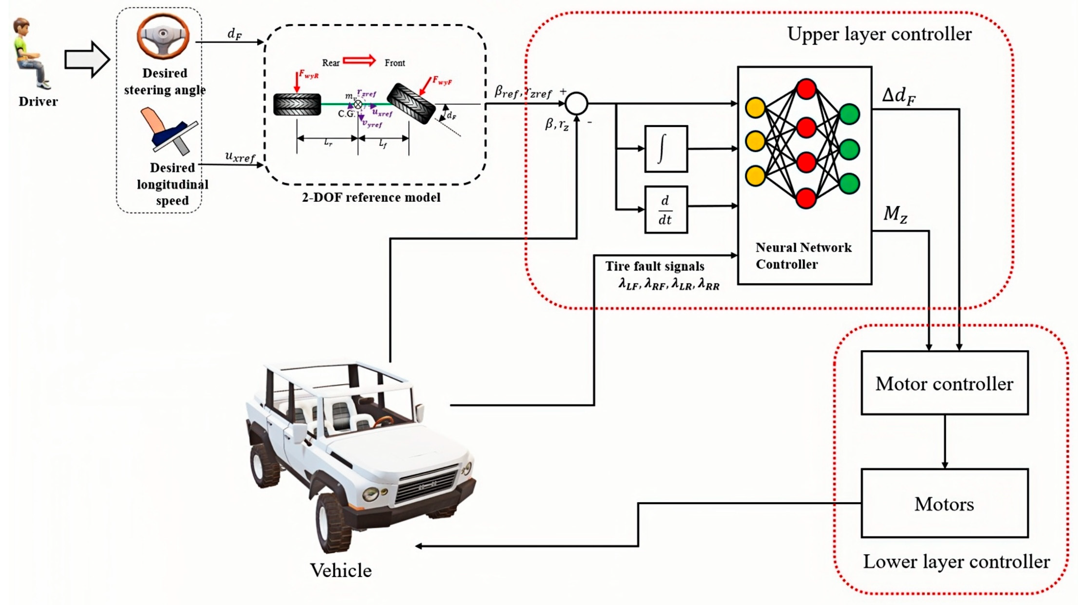
The proposed controller employs a collaborative architecture integrating ASC and DYC, as shown in Figure 1.

As shown in Figure 1, the controller comprises two distinct layers. Their functions and operational sequences are detailed below:

(a)

Upper-layer controller

The upper-layer controller integrates a 2-degree-of-freedom (2-DOF) reference model to calculate the desired extra front wheel steering angle (denoted as $\Delta d_F$) and yaw moment (denoted as $M_z$). The operation is as follows:

Step 1: Driver inputs (i.e., longitudinal speed and steering angle) are processed by the 2-DOF reference model to determine the desired yaw rate (denoted as $r_{zref}$) and side-slip angle (denoted as ${\beta }_{ref}$).

Step 2: The actual yaw rate (denoted as $r_z$) and side-slip angle (denoted as $\beta$) are continuously monitored. The system computes the error values, along with their integrals and derivatives.

Step 3: Tire blowout coefficients (${\lambda }_{LF}$, ${\lambda }_{RF}$, ${\lambda }_{LR}$, ${\lambda }_{RR}$) are incorporated into the neural network-based (NN-based) module. By processing error terms and blowout coefficients, the controller generates two key outputs: (1) the reference yaw moment $M_z$; and (2) the desired additional front wheel steering angle $\Delta d_F$. Finally, these are transmitted to the lower-layer controller.

(b)

Lower-layer controller

The lower-layer controller converts the upper-layer signals $M_z$ and $\Delta d_F$ into motor-specific control signals. The operation sequence is as follows:

Step 1: $M_z$ and $\Delta d_F$ values received from the upper layer are transformed into electrical signals (voltage and current).

Step 2: The converted signals are delivered to the rear wheel motor, enabling precise vehicle actuation and real-time stability control.

This dual-layer system ensures robust vehicle stability management during tire blowout scenarios. The dimension of the NN-based controller in the upper-layer controller is determined through training. The resulting architecture, which represents a significant evolution of our previous BCDA model, is defined as the broad critic extreme actor (BCEA).

3.2. Two-Degree-of-Freedom Reference Model

The primary objective of the control problem addressed in this study is to maintain stability during tire blowouts. The 2-DOF vehicle model is widely adopted in analysis of dynamics and provides a reference for controller design in this study. Consequently, the controller aims to meet the actual state of the vehicle with the reference state defined by the 2-DOF model, thereby ensuring optimal stability under tire blowout conditions.

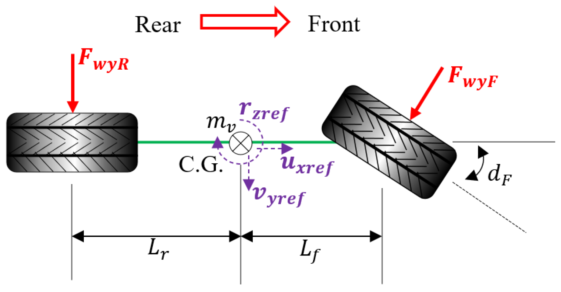
The 2-DOF reference model is derived from the Newton’s second law, as shown in Figure 2.

In Figure 2, $m_v$ represents the mass of the vehicle; $I_{zz}$ denotes the moment of inertia of the vehicle; $L_f$ and $L_r$ represent the distance from the center of gravity (C.G.) to the front and rear axles, respectively; and $d_F$ indicates the front wheel steering angle. The lateral tire forces for the front and rear wheels are denoted by $F_{wyF}$ and $F_{wyR}$, respectively. The reference longitudinal speed, lateral speed and yaw rate are represented by $u_{xref}$, $v_{yref}$ and $r_{zref}$, respectively.

The dynamic equation based on Newton’s second law is defined as

$$\{\begin{array}{c}{m}_v\left({\dot{v}}_{yref}+u_{xref}{r}_{zref}\right)=\sum F_y\\ I_{zz}{\dot{r}}_{zref}=\sum M_z\end{array},$$

(2)

where $\sum F_y$ and $\sum M_z$ represent the integral lateral force and yaw moment, respectively. These are calculated by

$$\{\begin{array}{c}\sum F_y=F_{yF}+F_{yR}\\ \sum M_z=L_f{F}_{yF}-L_r{F}_{yR}\end{array},$$

(3)

where $F_{yF}$ and $F_{yR}$ denote the lateral tire forces on the front and rear axles, respectively. These forces are calculated by

$$\{\begin{array}{c}{F}_{yF}=F_{wyF}\cos \left(d_F\right)\\ F_{yR}=F_{wyR}\end{array}.$$

(4)

Assuming small slip angles, the lateral tire forces are proportional to the tire slip angles. This linear relationship is expressed by

$$\{\begin{array}{c}{F}_{wyF}=C_f{\alpha }_F\\ F_{wyR}=C_r{\alpha }_R\end{array},$$

(5)

where $C_f$ and $C_r$ represent the cornering stiffness of the front and rear tires, respectively. The side-slip angles for front wheel ${\alpha }_F$ and rear wheel ${\alpha }_R$ are defined as

$$\{\begin{array}{c}{\alpha }_F={\tan }^{-1}\left({\displaystyle \frac{v_{yref}+L_f{r}_{zref}}{u_{xref}}}\right)-d_F\\ {\alpha }_R={\tan }^{-1}\left({\displaystyle \frac{v_{yref}-L_r{r}_{zref}}{u_{xref}}}\right)\end{array}.$$

(6)

The reference side-slip angle of the vehicle ${\beta }_{ref}$ is calculated by

$${\beta }_{ref}={\tan }^{-1}\left({\displaystyle \frac{U_y}{U_x}}\right)-{\theta }_{ref},$$

(7)

where ${\theta }_{ref}$ is the reference yaw angle of the vehicle and it is calculated by

$${\theta }_{ref}={{\displaystyle \int }}_0^t{r}_{zref}dt;$$

(8)

$U_x$ and $U_y$ represent the vehicle velocities in the global X and Y directions, respectively, and these velocities are calculated by

$$\{\begin{array}{c}{U}_x=u_{xref}\cos {\theta }_{ref}-v_{yref}\sin {\theta }_{ref}\\ U_y=u_{xref}\sin {\theta }_{ref}+v_{yref}\cos {\theta }_{ref}\end{array}$$

(9)

3.3. Design of BCEA Controller

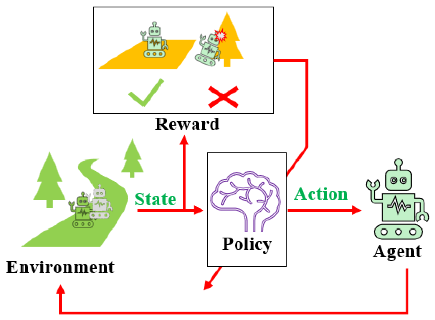
The fundamental process of RL is illustrated in Figure 3.

As shown in Figure 3, an RL system comprises four essential components. The first component is the agent, which is the central entity in the RL system. Next, the environment represents the external scenario in which the agent operates. The third component is the policy, which defines the decision-making rule. Finally, the reward signal serves as a feedback mechanism from the environment that evaluates the quality of the agent’s actions. This learning process is executed through a cyclic agent–environment interaction loop, as detailed below.

Step 1: Upon operating within the environment, the agent detects its current state, which includes speed and positional data.

Step 2: The detected state is processed by the policy to determine the required action using predefined computational methods.

Step 3: After the action is executed, the environment provides a reward signal based on the state transition and resulting outcome.

Step 4: With the objective of maximizing cumulative rewards, the agent updates its policy parameters.

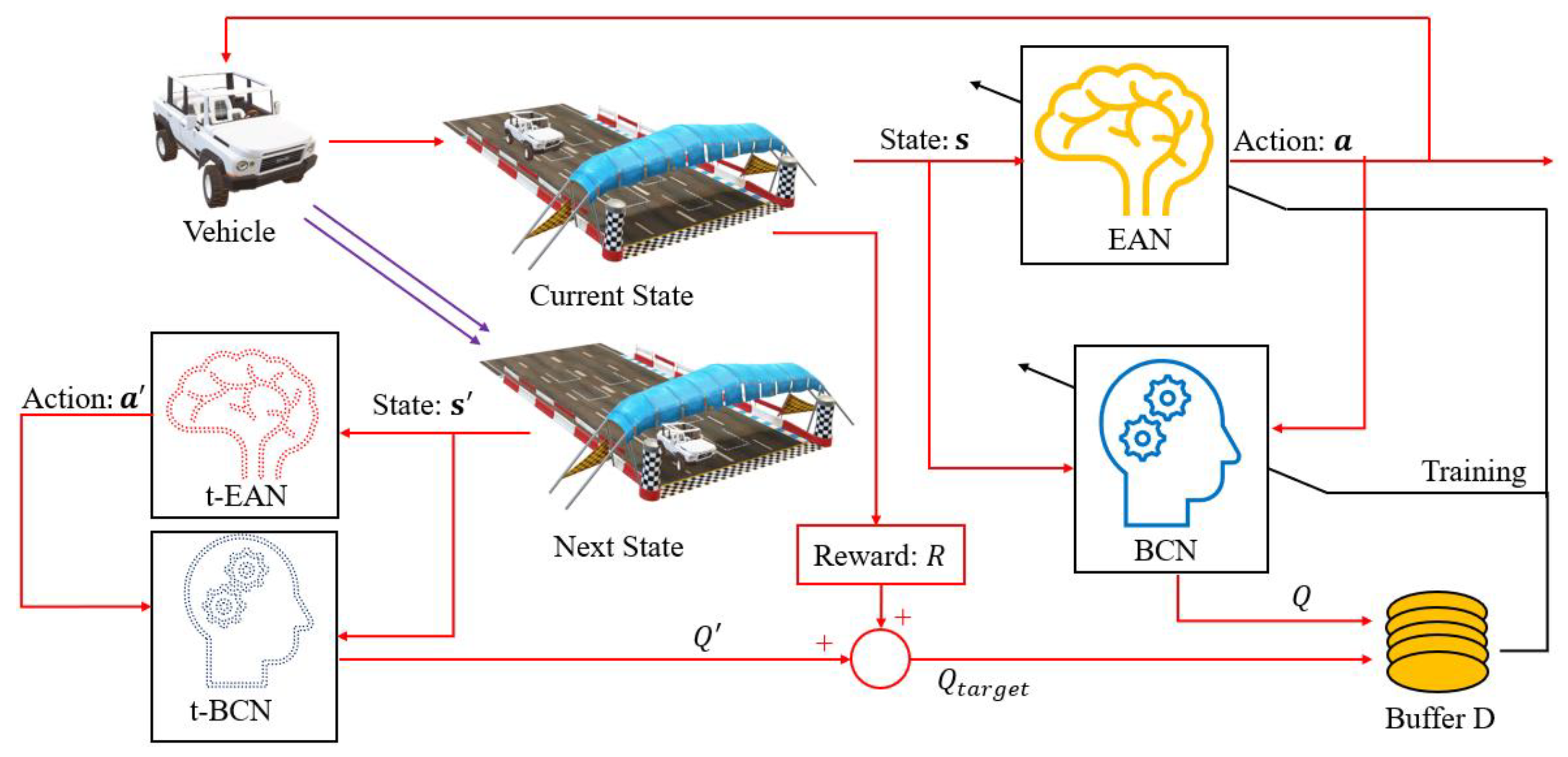
This iterative framework enables adaptive learning and optimal decision-making in dynamic environments. The flowchart of the proposed BCEA algorithm is illustrated in Figure 4 that integrates learning mechanisms to ensure robust performance across dynamic conditions.

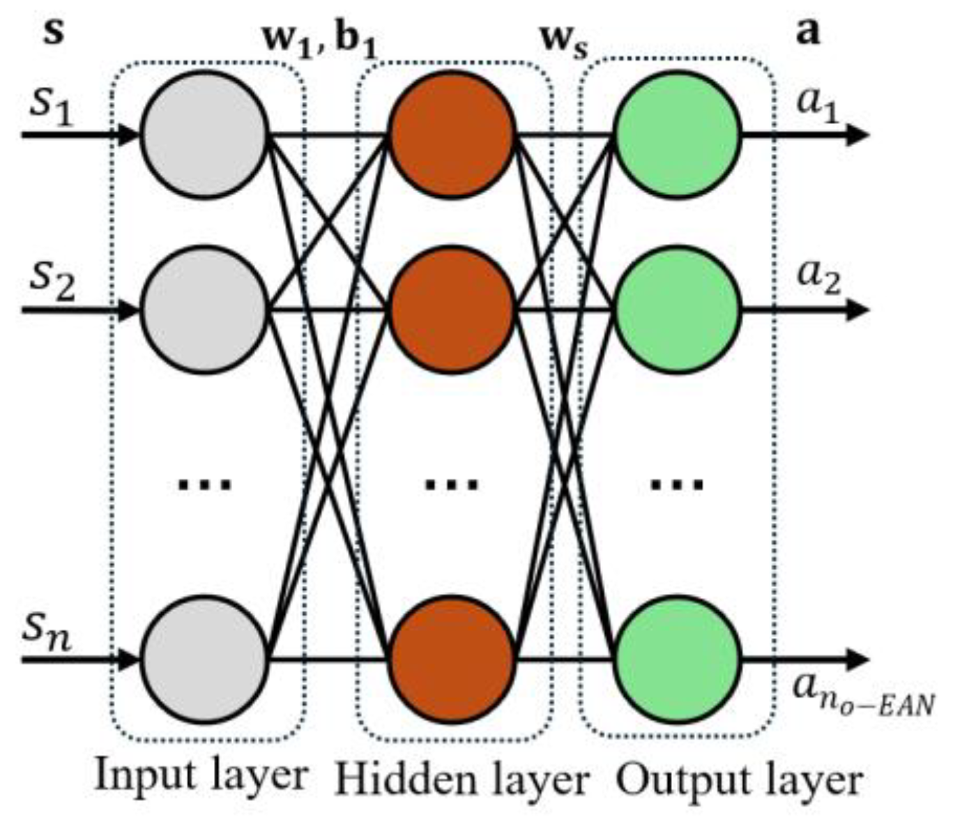
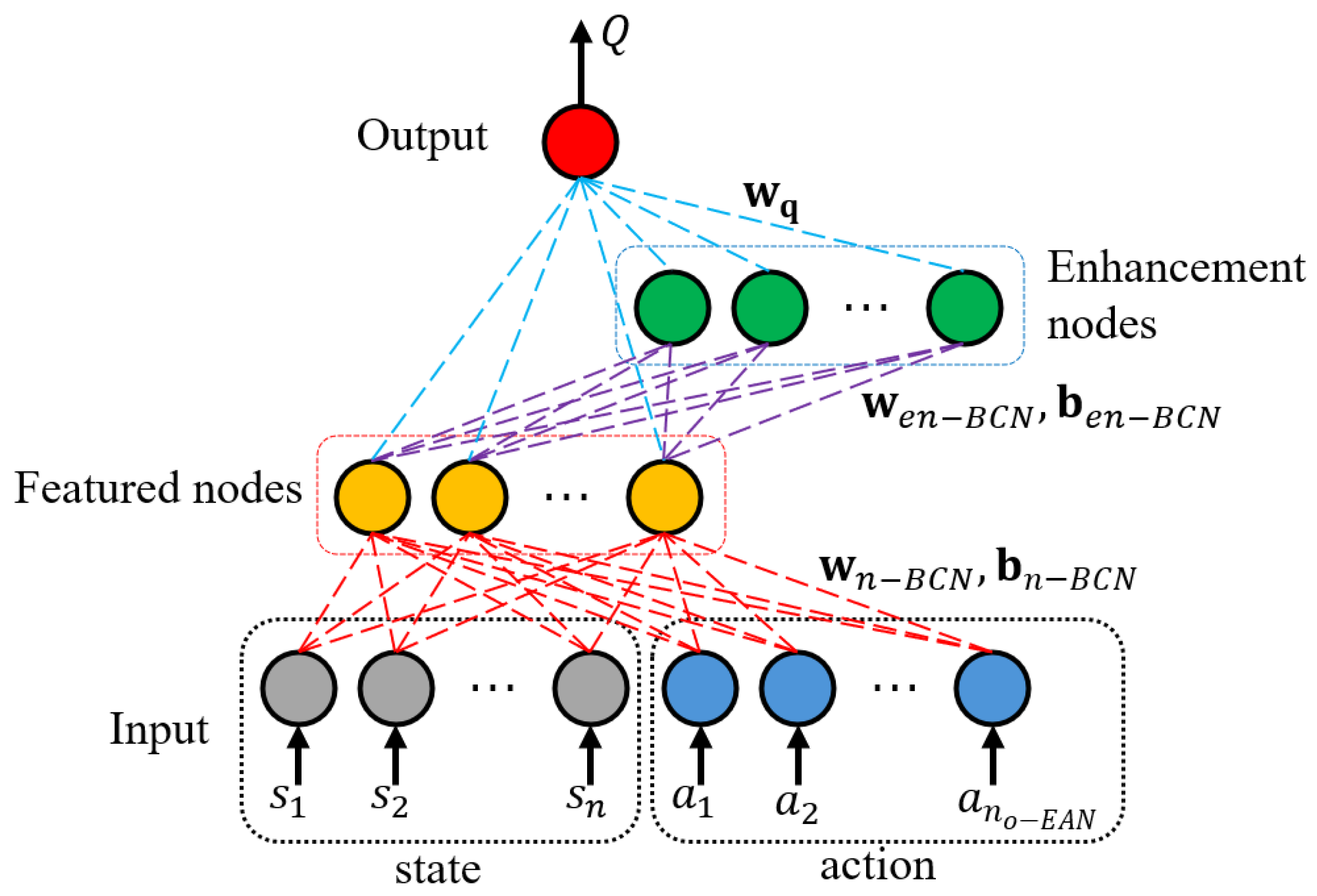
The BCEA architecture comprises four distinct networks. The first is the extreme actor network (EAN), which receives the state $s$ and outputs the action $a$. The EAN is structured as a single-hidden-layer neural network, with optimization performed using the extreme learning machine (ELM) algorithm. The second is the broad critic network (denoted as “BCN”), which receives both the state $s$ and action $a$ to output a Q-value, which evaluates the quality of the action. The BCN is designed based on the BLS, with its parameters optimized by the cuckoo search in this study. The third is the target EAN (denoted as “t-EAN”), which shares the same structure as the EAN. It calculates the next action $a^{\prime }$ based on the next state $s^{\prime }$. The fourth network is the target BCN (denoted as “t-BCN”), which is structurally similar to the BCN. The t-BCN calculates the Q-value of the predicted action $a^{\prime }$ (denoted as $Q^{\prime }$) by processing the next state $s^{\prime }$ and the predicted action $a^{\prime }$.

The training process proceeds sequentially. First, the reward (denoted as $R_s$) is calculated based on the current state $s$. The target Q-value (denoted as $Q_{target}$) is then computed using the Bellman equation by combining this reward with $Q^{\prime }$, which is generated based on the state on the next time step. The set consisting of state $s$, action $a$ and reward is stored in the experience replay buffer $\mathit{D}$. After a fixed number of iteration, random samples are retrieved from replay buffer $\mathit{D}$ to train BCN and EAN, optimizing their parameters to minimize error. The design of these networks is further discussed in the following sections.

3.3.1. Design of EAN

The architecture of the EAN is shown in Figure 5.

The EAN architecture comprises the input layer, the hidden layer, and the output layer. The implementation of a single hidden layer significantly improves computational efficiency. The input layer processes the state $s$ while the output layer generates the action $a$ based on the features extracted from the hidden layer. These outputs depend on the network parameters including the weight and bias matrices, denoted respectively as $w_{\mathbf{1}}$ and $b_{\mathbf{1}}$, which connect the input and hidden layers as illustrated in Figure 5. The state $s$ is composed of $n$ input variables as formulated by

$$s={\left[s_1,s_2,\dots ,s_n\right]}^T,$$

(10)

where $s_1,s_2,\dots ,s_n$ represent the variables in $s$.

In this study, the state $s$ is specifically defined to include tracking errors and tire fault signals, as expressed by

$$s={\left[\Delta r_z, \dot{\Delta }{r}_z,\int \Delta r_{z}dt, \Delta \beta ,\dot{\Delta }\beta ,\int \Delta \beta dt,{\lambda }_{LF},{\lambda }_{RF},{\lambda }_{LR},{\lambda }_{RR}\right]}^T,$$

(11)

where $\Delta r_z$ and $\Delta \beta$ represent the tracking errors of the yaw rate and side-slip angle, respectively; ${\lambda }_{LF}$, ${\lambda }_{RF}$, ${\lambda }_{LR}$ and ${\lambda }_{RR}$ denote the blowout coefficients for the left-front, right-front, left-rear and right-rear tires, respectively. The tracking errors $\Delta r_z$ and $\Delta \beta$ are defined as

$$\{\begin{array}{c}\Delta r_z=r_{zref}-r_z\\ \Delta \beta ={\beta }_{ref}-\beta \end{array}.$$

(12)

The inactivated hidden layer output matrix $H_{\mathbf{1}o}$ is calculated by

$$H_{\mathbf{1}o}=w_{\mathbf{1}}s+b_{\mathbf{1}}.$$

(13)

The activated neurons are then obtained by applying a nonlinear activation function $f\left(.\right)$, as expressed by

$$H_{\mathbf{1}}=f\left(H_{\mathbf{1}o}\right).$$

(14)

In this study, a Leaky ReLU function is selected as the activated function, as expressed by

$$f\left(x\right)=\{\begin{array}{c}x,if x\ge 0\\ {\lambda }_{k}x,if x<0\end{array}.$$

(15)

The reason for utilizing the Leaky ReLU is proposed in by (Wong et al., 2025) [53].

Finally, the EAN produces action $a$ which is computed by using the following weight matrix $w_s$:

$$a=w_s{H}_{\mathbf{1}}.$$

(16)

The action vector $a$ consists of the desired additional front wheel steering angle ($\Delta d_F$) and the desired yaw moment $M_z$:

$$a=\left[\Delta d_F, M_z\right]$$

(17)

3.3.2. Design of BCN

The BCN is proposed based on an optimized version of the original BCDA algorithm by [51]. To improve the stability and efficiency, a novel initialization strategy is proposed in which a substantial number of enhancement nodes are pre-configured, ensuring their count significantly exceeds that of the input layer nodes. Similarly, the number of featured nodes is maintained which is significantly larger than the input dimension. This strategy enables precise fitting during initialization, avoiding iterative calculations and enhancing the stability of the algorithm. The improved BCN architecture is illustrated in Figure 6.

The input for the BCN combines all the action and state vectors:

$$Z_{n-BCN}=\left[s_1,s_2,\dots ,s_{n_{s-BCN}},a_1,a_2,\dots ,a_{n_{o-EAN}}\right]$$

(18)

Let $w_{n-BCN}$ and $b_{n-BCN}$ denote the weight and bias matrices that map inputs to feature nodes. Thus, the inactivated feature nodes are calculated by

$$H_{of-BCN}=w_{n-BCN}{Z}_{n-BCN}+b_{n-BCN}$$

(19)

Applying the activation function from Equation (15), the featured nodes become

$$H_{f-BCN}=f\left(H_{of-BCN}\right)$$

(20)

Subsequently, the enhancement nodes are generated by the using the weights $w_{en-BCN}$ and $b_{en-BCN}$:

$$H_{oen-BCN}=w_{en-BCN}{H}_{f-BCN}+b_{en-BCN}$$

(21)

Applying Equation (14), the enhancement nodes become

$$H_{en-BCN}=f\left(H_{oen-BCN}\right)$$

(22)

Combining the featured and enhancement nodes yields the comprehensive hidden layer matrix $Z^h$:

$$Z^h=\left[\begin{array}{c}{H}_{f-BCN}\\ H_{en-BCN}\end{array}\right]$$

(23)

The final output Q-value is computed by

$$Q=w_q{Z}^h,$$

(24)

where $w_q$ is the output weight matrix.

3.3.3. Design of Target Networks (t-EAN and t-BCN)

The target network architecture comprises the t-EAN and t-BCN. The t-EAN retains an identical structure to the EAN. When the vehicle executes action $a$, the t-EAN computes the predicted next action $a^{\prime }$ based on the subsequent state $s^{\prime }$. Similarly, the t-BCN mirrors the structure of the BCN. It processes the anticipated state $s^{\prime }$ and predicted action $a^{\prime }$ to generate the estimated target Q-value $Q^{\prime }$. The coordination of these target networks enables stable prediction of future system behavior, which is essential to effective vehicle control.

3.4. Training of BCEA

3.4.1. Computation of Target Q-Value

An appropriately designed reward function is critical for evaluating system performance in safety-critical RL applications. Since trajectory stability is very important in this study, the reward focuses on minimizing tracking errors rather than maximizing the computational speed. The reward function $R_s$ is defined as

$$R_s={\displaystyle \frac{1}{\epsilon +\sqrt{{\left(X-X_{ref}\right)}^2+{\left(Y-Y_{ref}\right)}^2}}}$$

(25)

where ($X, Y$) and ($X_{ref},Y_{ref}$) represent the trajectory coordinates of the actual vehicle and the 2-DOF reference model, respectively. $\epsilon$ is a small positive constant to prevent division by zero.

The target Q-value is computed using the Bellman equation:

$$Q_{target}=R_s+\gamma Q^{\prime },$$

(26)

where $\gamma \in \left[0,1\right]$ is the discount factor, and $Q^{\prime }$ is the estimated Q-value for the next state.

3.4.2. Training of BCN

Let $d$ be the batch size of the training data. The input matrix to the BCN, $Z_{n-BCN}^d$, is formed by concatenating $d$ training samples, as expressed by

$$Z_{n-BCN}^d=\left[\begin{array}{cccc}{Z}_{n-BCN}^{\left(1\right)}& Z_{n-BCN}^{\left(2\right)}& \dots & Z_{n-BCN}^{\left(d\right)}\end{array} \right].$$

(27)

For the $i$-th sample ($1\le i\le d$), the input is $Z_{n-BCN}^{\left(i\right)}={\left[s_i,a_i\right]}^T$. The inactivated feature nodes are calculated by

$$H_{of-BCN}^{\left(i\right)}=w_{n-BCN}{Z}_{n-BCN}^{\left(i\right)}+b_{n-BCN}$$

(28)

The activated feature nodes are obtained by

$$H_{f-BCN}^{\left(i\right)}=f\left(H_{of-BCN}^{\left(i\right)}\right),$$

(29)

where $f\left(.\right)$ is the Leaky ReLU function as expressed in Equation (17).

Subsequently, the enhancement nodes are generated by

$$H_{oen-BCN}^{\left(i\right)}=w_{en-BCN}{H}_{f-BCN}^{\left(i\right)}+b_{en-BCN},$$

(30)

where $w_{en-BCN}$ and $b_{en-BCN}$ are the weights and biases for the enhancement nodes in the BCN, respectively.

$$H_{en-BCN}^{\left(i\right)}=f\left(H_{oen-BCN}^{\left(i\right)}\right).$$

(31)

The complete hidden layer vector for the $n$-th sample combining both feature and enhancement nodes and is shown below:

$$Z^{{\mathit{h}}^{\left(i\right)}}=\left[\begin{array}{c}{H}_{f-BCN}^{\left(i\right)}\\ H_{en-BCN}^{\left(i\right)}\end{array}\right].$$

(32)

Aggregating all samples in the batch yields the matrix $Z_{m-BCN}^d$ as expressed by

$$Z_{m-BCN}^d=\left[\begin{array}{cccc}{H}_{f-BCN}^{\left(1\right)}& H_{f-BCN}^{\left(2\right)}& \dots & H_{f-BCN}^{\left(d\right)}\\ H_{en-BCN}^{\left(1\right)}& H_{en-BCN}^{\left(2\right)}& \dots & H_{en-BCN}^{\left(d\right)}\end{array}\right].$$

(33)

The target output vector $Y$ consists of the target Q-values for each sample, as expressed by

$$Y=\left[\begin{array}{c}{Q}_{target}^{\left(1\right)}\\ Q_{target}^{\left(2\right)}\\ \dots \\ Q_{target}^{\left(d\right)}\end{array}\right],$$

(34)

where $Q_{target}^{\left(1\right)}$, $Q_{target}^{\left(2\right)}$, …, $Q_{target}^{\left(d\right)}$ represent the target Q-values of the training sets.

The output weight matrix $w_q$ is then calculated analytically using the following pseudoinverse:

$$w_q=Y{\left(Z_{m-BCN}^d\right)}^{†}.$$

(35)

where the pseudoinverse ${\left(Z_{m-BCN}^d\right)}^{†}$ is defined using ridge regression regularization as shown in

$${\left(Z_{m-BCN}^d\right)}^{†}=\left(\underset{\lambda \to 0}{\lim }{\left({{\mathit{Z}}_{m-BCN}^d}^T{Z}_{m-BCN}^d+\lambda I\right)}^{-1}\right){Z_{m-BCN}^d}^T.$$

(36)

3.4.3. Training of EAN

(a)

Training of target actions

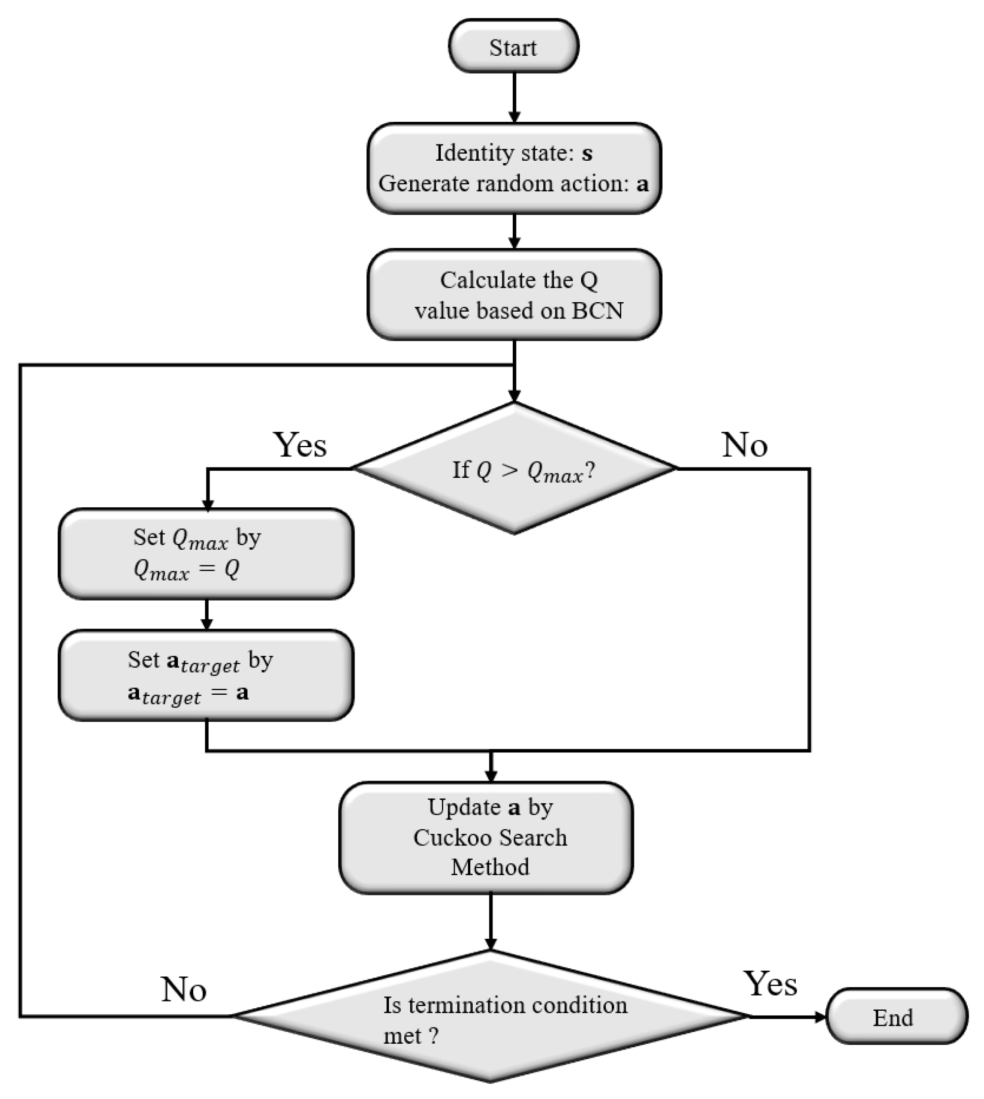
Once the BCN structure is fixed, the Q-value depends solely on the action $a$ for a given state $s$. To maximize the Q-value, a meta-heuristic approach is employed rather than gradient ascent. The cuckoo search (CS) algorithm is selected because of its simplicity and effectiveness [57]. The target action $a$ is optimized to maximize the Q-value while keeping $s$ constant as illustrated in Figure 7.

(b)

Training of EAN parameters

The parameters of the EAN are updated using the ELM method. For a training batch of size $d$, with the states set as $s_1$, $s_2$, …, $s_d$ and optimized target actions as $a_{1t}$, $a_{2t}$, …,$a_{dt}$, the aggregate matrices are

$$s_t=\left[\begin{array}{c}{s}_1\\ s_2\\ \dots \\ s_d\end{array}\right], a_t=\left[\begin{array}{c}{a}_{1t}\\ a_{2t}\\ \dots \\ a_{dt}\end{array}\right]$$

(37)

The inactivated hidden layer neurons for the $i$-th sample in $s_t$ are

$${\mathit{H}}_{\mathbf{1}\mathbf{o}}^{\left(i\right)}=w_1{\mathit{s}}_{\mathit{i}}+b_{\mathbf{1}},$$

(38)

where $w_1$ and $b_{\mathbf{1}}$ are the weights and biases in the EAN, respectively.

Applying the activation function yields

$${\mathit{H}}_{\mathbf{1}}^{\left(i\right)}=f\left({\mathit{H}}_{\mathbf{1}\mathbf{o}}^{\left(i\right)}\right)$$

(39)

The hidden layer matrix $H_{\mathit{t}\mathit{r}}$ combines neurons from all training samples, as expressed by

$$H_{\mathit{t}\mathit{r}}=\left[\begin{array}{cccc}{H}_1^{\left(1\right)}& H_1^{\left(2\right)}& \dots & H_1^{\left(d\right)}\end{array}\right]$$

(40)

The output weight matrix ${\mathit{w}}_{\mathit{s}}$ is then computed by the pseudoinverse:

$${\mathit{w}}_{\mathit{s}}=a_t{\left(H_{\mathit{t}\mathit{r}}\right)}^{†}.$$

(41)

3.4.4. Updating Target Networks

The parameters of the t-BCN (${\theta }_{t-BCN}$) and t-EAN (${\theta }_{t-EAN}$) are updated by using a soft update rule after each episode:

$$\{\begin{array}{c}{\theta }_{t-BCN}^{\prime }={\lambda }_b{\theta }_{t-BCN}+\left(1-{\lambda }_b\right){\theta }_{BCN}\\ {\theta }_{t-EAN}^{\prime }={\lambda }_e{\theta }_{t-EAN}+\left(1-{\lambda }_e\right){\theta }_{EAN}\end{array},$$

(42)

where ${\lambda }_{b,}{\lambda }_e\in \left[0,1\right]$ are the soft update coefficients; ${\theta }_{t-BCN}$ and ${\theta }_{t-EAN}$ represent the parameters of the original t-BCN and t-EAN, respectively; and ${\theta }_{BCN}^{\prime }$ and ${\theta }_{EAN}^{\prime }$ denote the parameters of the updated BCN and EAN.

The stability of the proposed BCEA algorithm is analyzed via a Lyapunov function during and after training. Hardware restrictions (e.g., battery voltage, maximum front wheel steering angle) are considered for training. The BCEA training algorithm is summarized in Algorithm 1.

Algorithm 1: Training of BCEA controller

Randomly initialize ${\theta }_{BCN}$ and ${\theta }_{EAN}$;

Initialize target parameters: ${\theta }_{t-BCN}={\theta }_{BCN}$ and ${\theta }_{t-EAN}={\theta }_{EAN}$;

Initialize replay buffer $D$;

for episode = 1 to M do:

Update ${\theta }_{t-EAN}$ and ${\theta }_{t-BCN}$ using Equation (42).

for $t=1$ to $N$ do:

Observe current state $s_t$;

Calculate the reward $R_s$ using Equation (25);

Select action $a_t$ using EAN;

Execute action $a_t$ and observe next state $s^{\prime }$;

Compute predicted action $a^{\prime }$ using t-EAN;

Compute predicted Q-value $Q\left(s^{\prime }, a^{\prime }\right)$ using t-BCN;

Calculate $Q_{target}$ using Equation (26);

Store tuple ($s$, $a$, $Q_{target}$) in replay buffer $D$;

if buffer $D$ has sufficient samples (e.g., when samples = 1000) then:

Randomly sample batch $s_1$, $s_2$…, $s_d$, $a_1$,$a_2$, …, $a_d$ and $Q_{target}^{\left(1\right)}$, $Q_{target}^{\left(2\right)}$, …, $Q_{target}^{\left(d\right)}$ from D;

Update ${\theta }_{BCN}$ using Equations (27)–(36);

Optimize target actions using CS (as shown in Figure 7).

Update ${\theta }_{EAN}$ using Equations (37)–(41);

end if

end for

end for

3.5. Design of Lower- Layer Controller

The lower-layer controller translates the stability targets into physical actuator commands [51]. First, the relationship between the front wheel steering angle and the rotor displacement of steering motor is defined as

$${\theta }_{sm}=g_{sm}\left(\Delta d_F,d_F\right)$$

(43)

where ${\theta }_{sm}$ is the angular displacement of the steering motor rotor, and $g_{sm}\left(.\right)$ is a kinematic function determined by the specific mechanical design of the steering system. $d_F$ represents the current front wheel steering angle, while $\Delta d_F$ is the compensated steering angle calculated by the BCEA controller.

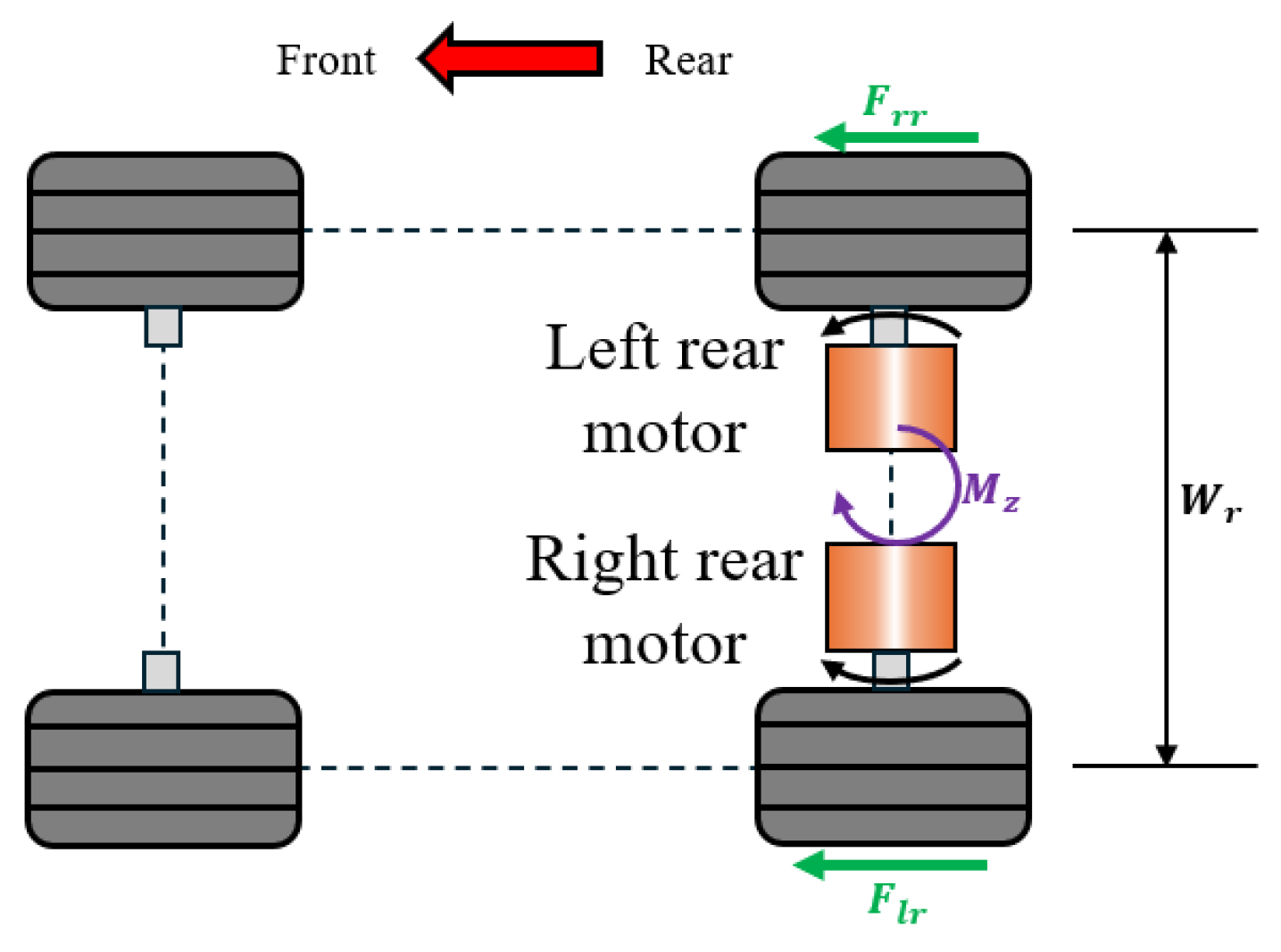
The desired yaw moment is generated via differential driving of the left- and right- rear independent drive motors, as illustrated in Figure 8.

The relationship between the desired yaw moment $M_z$ and the rear-wheel-drive forces is given by

$$M_z={\displaystyle \frac{1}{2}}{W}_r\left(\left(1-{\lambda }_{LR}\right)F_{lr}-\left(1-{\lambda }_{RR}\right)F_{rr}\right),$$

(44)

where $W_r$ is the wheel track, and $F_{lr}$ and $F_{rr}$ are the drive forces of the left- and right-rear wheels, respectively.

Additionally, the total longitudinal force must satisfy the acceleration demand of the driver:

$$\left(1-{\lambda }_{LR}\right)F_{lr}+\left(1-{\lambda }_{RR}\right)F_{rr}=F_{xrreq},$$

(45)

where $F_{xrreq}$ is the total desired longitudinal force determined by the accelerator pedal position.

By solving Equations (46) and (47) simultaneously, the required drive forces for each wheel are derived as

$$\left[\begin{array}{c}{F}_{lr}\\ F_{rr}\end{array}\right]=\left[\begin{array}{c}{\displaystyle \frac{1}{2\left(1-{\lambda }_{LR}+ϵ\right)}}{F}_{xrreq}+{\displaystyle \frac{M_z}{W_r\left(1-{\lambda }_{LR}+ϵ\right)}}\\ {\displaystyle \frac{1}{2\left(1-{\lambda }_{RR}+ϵ\right)}}{F}_{xrreq}-{\displaystyle \frac{M_z}{W_r\left(1-{\lambda }_{LR}+ϵ\right)}}\end{array}\right],$$

(46)

where $ϵ$ is a small positive constant added to prevent division by zero during tire blowout (i.e., when ${\lambda }_i\approx 1$).

Finally, the target output torque for each motor ($T_{el{r}_{des}}$ and $T_{er{r}_{des}}$) is calculated by multiplying the required forces by the wheel radius $R_w$, as expressed by

$$\left[\begin{array}{c}{T}_{el{r}_{des}}\\ T_{er{r}_{des}}\end{array}\right]=\left[\begin{array}{c}{F}_{lr}\\ F_{rr}\end{array}\right]R_w=\left[\begin{array}{c}{\displaystyle \frac{1}{2\left(1-{\lambda }_{LR}+ϵ\right)}}{F}_{xrreq}{R}_w+{\displaystyle \frac{M_z{R}_w}{W_r\left(1-{\lambda }_{LR}+ϵ\right)}}\\ {\displaystyle \frac{1}{2\left(1-{\lambda }_{LR}+ϵ\right)}}{F}_{xrreq}{R}_w-{\displaystyle \frac{M_z{R}_w}{W_r\left(1-{\lambda }_{LR}+ϵ\right)}}\end{array}\right],$$

(47)

4. Simulation and Prototype Tests

4.1. Prototype Development

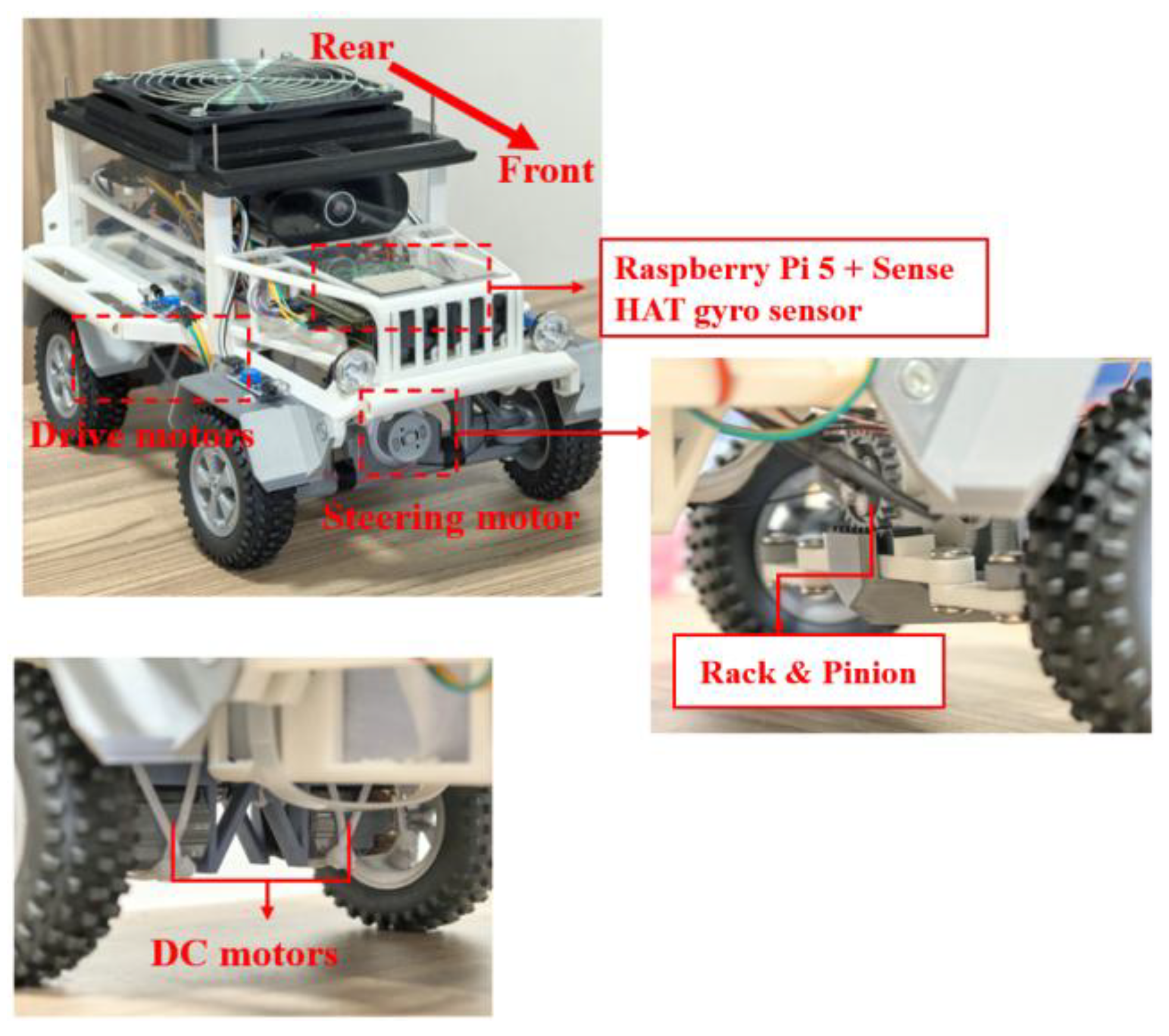
The prototype is regarded as an effective method for testing and verifying the controllers, as indicated by the research of [60,61]. To verify the effectiveness of the proposed controller, a scaled electric vehicle prototype is developed, as shown in Figure 9.

The body of the prototype is constructed using 3D-printed parts. The steering system is actuated by a ZX300 DC servo motor, while the rear wheels are independently driven by two 8883-EX DC motors. The physical parameters of the prototype are measured experimentally and listed in

Table 1. Parameters of prototype vehicle.

Parameter	Symbol	Value
Mass	$m_s$	2.06 $\mathrm{k}\mathrm{g}$
Moment of inertia	$I_{zz}$	0.017 $\mathrm{k}\mathrm{g}·{\mathrm{m}}^2$
Distance from front axle to C.G.	$L_f$	$0.114 \mathrm{m}$
Distance from rear axle to C.G.	$L_r$	$0.066 \mathrm{m}$
Wheel radius	$R_w$	Before tire blowout: 0.0375 $\mathrm{m}$ After tire blowout: 0.022 $\mathrm{m}$
Cornering stiffness of front wheels	$C_f$	Before tire blowout: 5.58 $\mathrm{N}/\mathrm{rad}$ After tire blowout: 1.19 $\mathrm{N}/\mathrm{rad}$
Cornering stiffness of rear wheels	$C_r$	Before tire blowout: 9.82 $\mathrm{N}/\mathrm{rad}$ After tire blowout: 2.04 $\mathrm{N}/\mathrm{rad}$
Wheel track	$W_r$	0.164 $\mathrm{m}$

.

In both the prototype and the model, a tire is considered a blowout tire when the air pressure of the tire falls below a set threshold $P_s$. This definition applies regardless of the speed of pressure decay. Once the tire pressure is detected below $P_s$, the fault detection is activated immediately. In MATLAB 2020a simulation, the dynamic process of a tire blowout is simulated with the Dugoff tire model according to [60,61,62]. Tire parameters are directly adjusted to represent the dynamic changes in the vehicle after a blowout. In prototype vehicle tests, a pre-set blown-out tire is installed to physically simulate a tire blowout because the development of a remote-controlled actuator for sudden tire blowout is challenging.

The electrical parameters and the controllers of the independent drive motors are detailed in [53], as shown in

Table 2. Parameters of electric motors.

Parameter	Value
Winding resistance	29.59 $\mathsf{\Omega }$
Winding inductance	2.78 H
Back EMF coefficient	0.091 $\mathrm{V}·\mathrm{s}$
Torque constant	0.175 $\mathrm{N}·\mathrm{m}·{\mathrm{A}}^{-1}$
Damping coefficient	0.0005 $\mathrm{N}·\mathrm{m}·\mathrm{s}$

.

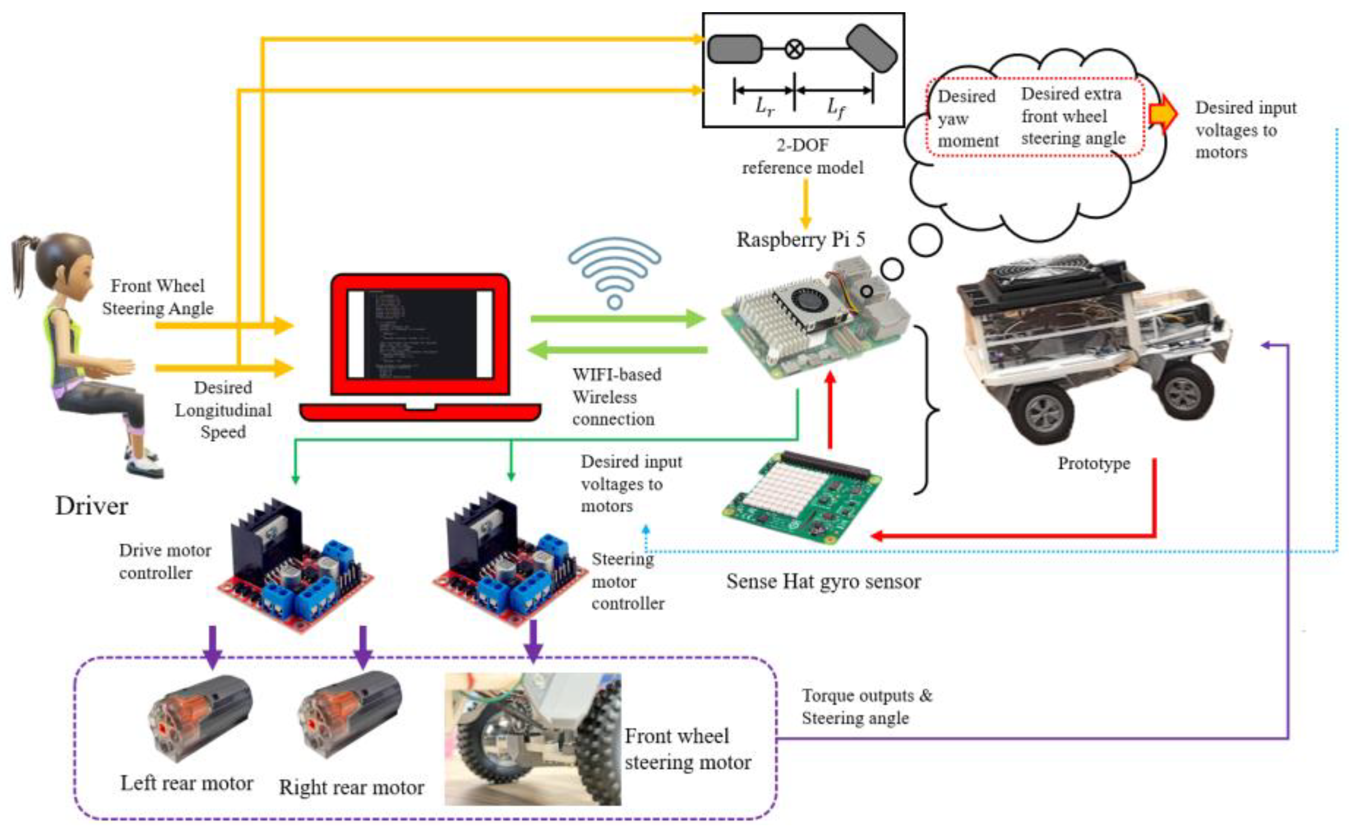
The Pulse Width Modulation (PWM) frequency of the motor controller is set as 30 Hz. The control system is implemented on a Raspberry Pi 5, which processes vehicle motion data captured by a Sense HAT gyroscope. The accuracies of the gyroscope sensors are within ±10%. The 2-DOF reference model and the BCEA control algorithm are executed locally on the Raspberry Pi using Python 3.9.2.

The system operates via a WIFI-based hardware-in-the-loop configuration. A remote laptop captures driver inputs (i.e., desired longitudinal speed and steering angle) and transmits them to the Raspberry Pi 5. The Raspberry Pi 5 calculates the required extra steering angle and yaw moment and then converts them into motor voltages and drives the motors to execute the maneuver. This architecture is illustrated in Figure 10.

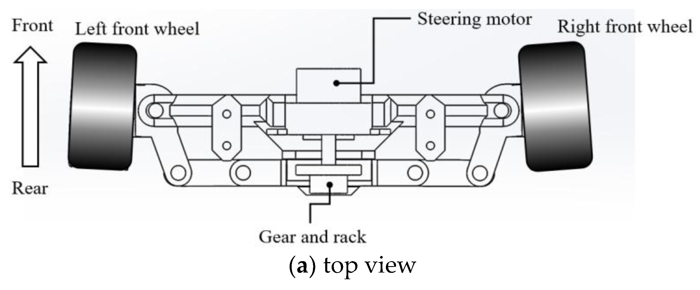
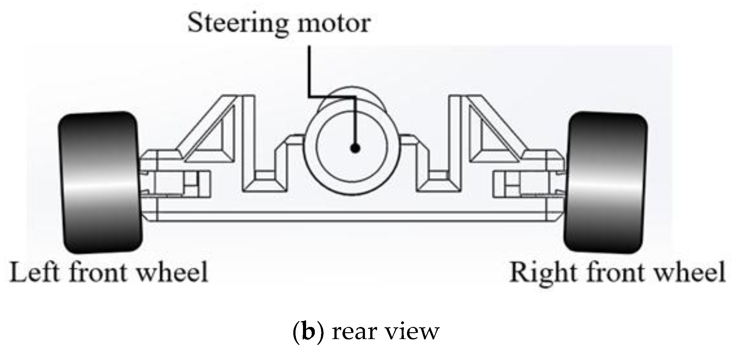
The prototype utilizes an Ackermann steering geometry, as depicted in Figure 11a,b.

Equation (43) is designed according to [53]. The training phase is conducted in MATLAB 2020a. To comprehensively evaluate the controller, the validation scenarios are divided into two categories: (a) sudden tire blowout during high speed and (b) restarting the vehicle from a standstill after a tire blowout. Due to the safety risks and limitations of inducing sudden structural tire failure on the scaled prototype, high-speed blowout dynamics is verified via simulation. The capability of the controller to stabilize and restart the vehicle from a standstill under persistent blowout condition is validated through physical road test with the scaled prototype.

4.2. MATLAB-Based Simulation Environment

4.2.1. Vehicle Modeling

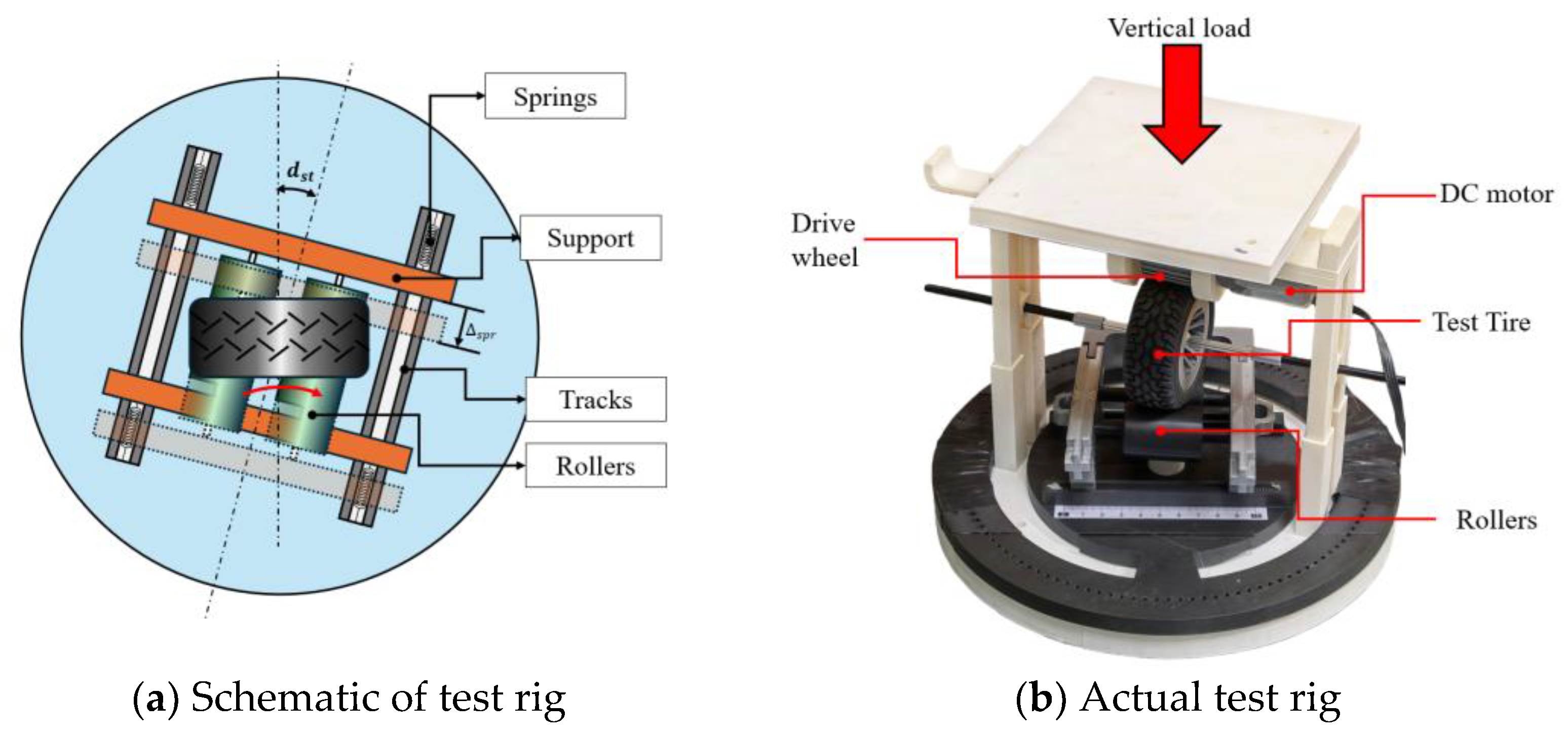
The dynamic model of the prototype is established based on the Dugoff tire model proposed in [62,63,64]. The air pressure of a healthy tire is defined as 0.2 bar for the prototype. The threshold pressure $P_s$ is consequently defined as 0.1 bar, representing a 50% reduction from the healthy tire pressure [65]. The parameters are acquired directly from the physical prototype with the test rig shown in Figure 12.

The parameters used in the Dugoff tire model for both blown-out and healthy tires are measured through the test rig shown in Figure 12. The Dugoff tire model requires parameters for vertical stiffness, radius, longitudinal slip stiffness and cornering stiffness. According to the research of [66,67], a blown-out tire retains approximately 6.7% of the vertical stiffness, 70% of the radius, 28% of the longitudinal slip stiffness, and 25% of the cornering stiffness of a healthy tire. In this study, the measured vertical stiffness, radius, longitudinal slip stiffness, front wheel lateral stiffness and rear wheel lateral stiffness of a normal wheel are 335.46 N/m, 0.0375 m, 884.3 N/m, 5.58 N/rad, and 9.82 N/rad, respectively. For a blown-out tire, the corresponding parameters are 18.34 N/m, 0.022 m, 206.2 N/m, 1.19 N/rad, and 2.04 N/rad, respectively. Consequently, the ratios of the blown-out parameters to the healthy parameters are 5.47% for vertical stiffness, 58.67% for radius, 23.32% for longitudinal slip stiffness, 21.33% for front wheel cornering stiffness, and 20.77% for rear wheel cornering stiffness. These parameters align closely with the requirements outlined in [66,67]. Thus, the Dugoff tire model utilized in this study can reflect the authenticity of the experimental results.

In the MATLAB simulation, the vertical stiffness decreases from 335.46 N/m to 18.34 N/m. The radius reduces from 0.0375 m to 0.022 m. The longitudinal slip stiffness drops from 884.3 N/m to 206.2 N/m. Additionally, the cornering stiffnesses of the front and rear tires change from 5.58 N/rad and 9.82 N/rad to 1.19 N/rad and 2.04 N/rad, respectively.

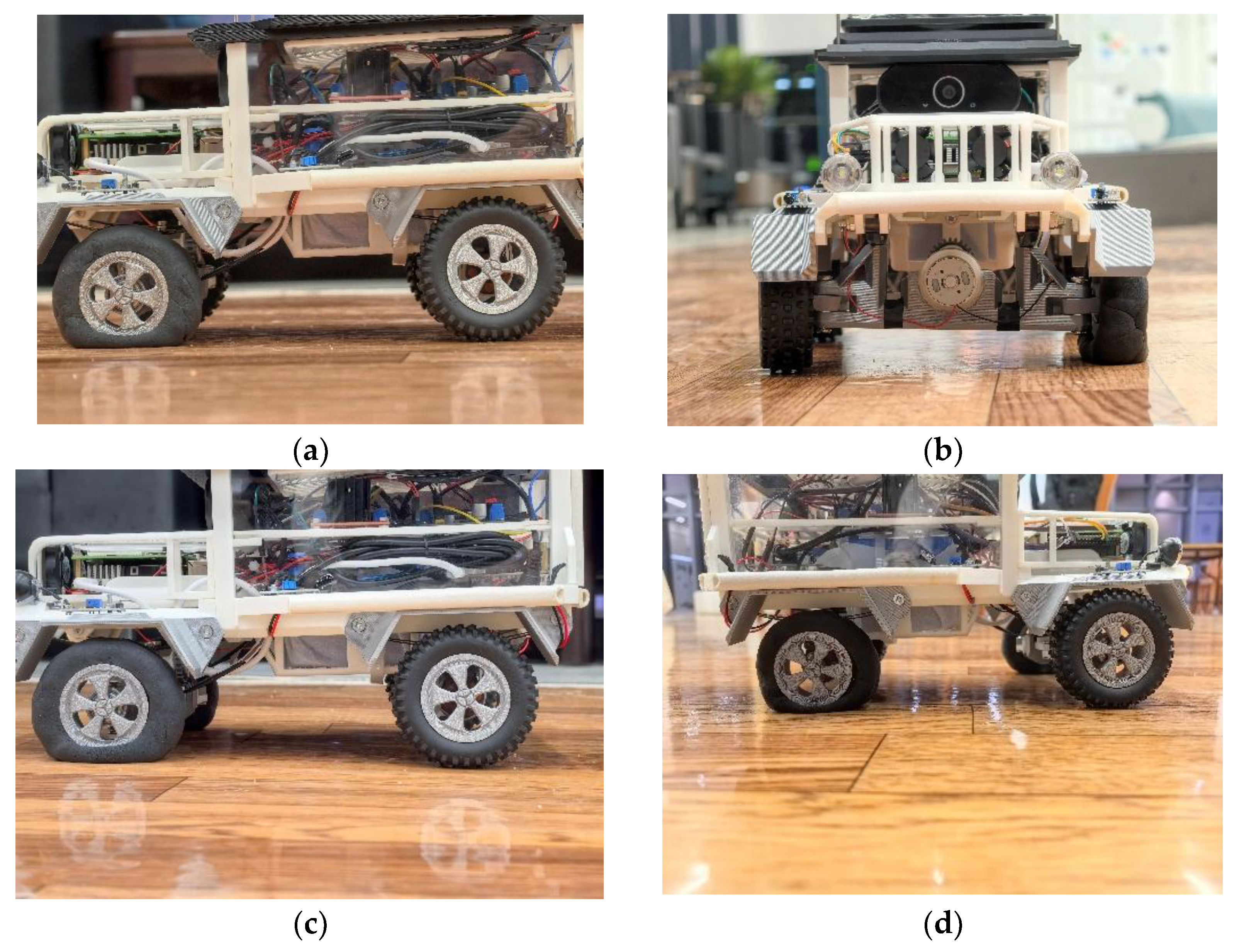
To ensure that the model can accurately reflect real failure modes, the prototype is physically configured and tested under two tire blowout scenarios. These configurations include left-front tire blowout (denoted as “LF”) and simultaneous blowouts of the left-front and right-rear tires (denoted as “LF+RR”), as illustrated in Figure 13.

The energy released during a tire blowout is calculated by

$$\delta E=\overline{P}\Delta V ,$$

(48)

where $\delta E$ represents the energy loss of the blown-out tire, $\overline{P}$ represents the average air pressure of the tire during the blowout process, and $\Delta V$ represents the volumetric change in the air in the tire. In the prototype, $\overline{P}$ equals 0.15 bar and $\Delta V$ equals 0.86 × 10⁻⁵ m³. Thus, $\delta E$ is approximately 0.13 J. This energy value is minimal and can be considered negligible in the context of the lateral dynamics.

4.2.2. Training Process and Stability Analysis

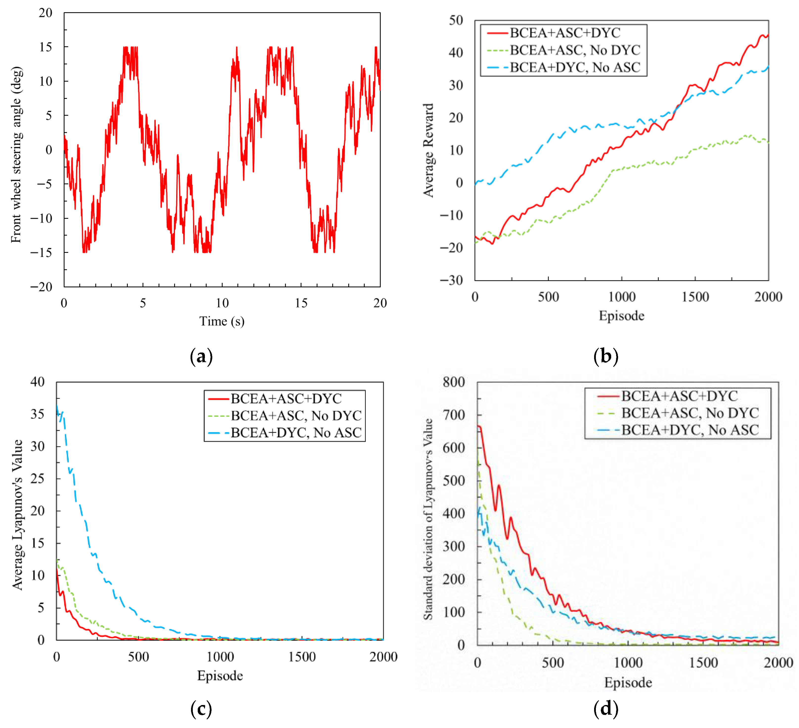
During each training episode, the vehicle is subjected to randomized, continuous steering signals to simulate diverse driving intentions (see Figure 14a for example). The vehicle speed is maintained at a constant 1.5 m/s, which corresponds to a full-scale vehicle speed of approximately 90 km/h. At the beginning of each training episode, the conditions of tire blowouts are randomly set. These conditions include the number of blown-out tires (one or two), the positions of these tires, and the time of blowout. The time of blowout is randomly selected between 0 and 20 s.

To ensure system stability, a Lyapunov function $L$ is defined based on the tracking errors:

$$L={\displaystyle \frac{1}{2}}\Delta r_z^2+{\displaystyle \frac{1}{2}}\Delta {\beta }^2$$

(49)

Utilizing Lyapunov’s method, the stability criteria for the training process are twofold:

(a)

For any non-zero errors $\Delta r_z$ and $\Delta \beta$, the function $L$ must be non-negative ($L\ge 0$).

(b)

Throughout the training process, the average value of $L$ must exhibit a decreasing trend, with its standard deviation remaining within a bounded range.

To train the controller for robustness, tire blowout scenarios are introduced stochastically. A maximum of two tires is randomly applied to one episode, with a random timing and wheel locations. The training and testing scenarios encompass two distinct failure categories (“LF” blowout and “LF+RR” blowout).

To verify the training efficiency of the BCEA, three configurations are implemented and evaluated, including BCEA for ASC only (denoted as “BCEA+ASC, No DYC”), BCEA for DYC only (denoted as “BCEA+DYC, No ASC”) and BCEA for both ASC and DYC (denoted as “BCEA+ASC+DYC”).

The training framework is implemented in MATLAB. The key hyperparameters include 100 hidden nodes for the EAN, 36 featured nodes and 1080 enhancement nodes for the BCN. The training duration is set to 2000 episodes.

The input of front wheel steering angle is shown in Figure 13a. The selection of 2000 episodes represents an optimal balance between performance and computational efficiency. As listed in

Table 3. Training performance metrics for BCEA at various stages.

No. of Episodes	Controller Configuration	Average Reward	Average Lyapunov Value	Standard Deviation of Lyapunov Value
1	BCEA+ASC+DYC	−16.12	11.13	669.62
	BCEA+ASC, no DYC	−18.3	12.78	597.27
	BCEA+DYC, no ASC	−1.49	36.66	407.51
500	BCEA+ASC+DYC	−3.93	0.267	136.53
	BCEA+ASC, no DYC	−12.33	0.663	21.84
	BCEA+DYC, no ASC	14.63	3.565	103.75
1000	BCEA+ASC+DYC	14.23	0.152	45.729
	BCEA+ASC, no DYC	4.743	0.217	3.409
	BCEA+DYC, no ASC	17.21	0.613	45.723
2000	BCEA+ASC+DYC	45.53	0.251	15.69
	BCEA+ASC, no DYC	12.467	0.184	4.778
	BCEA+DYC, no ASC	35.91	0.316	26.617

, insufficient training leads to poor control performance. Conversely, exceeding 2000 episodes yields negligible performance gains.

The training process and results are shown in Figure 13b–d. The average reward demonstrates a continuous upward trend, while the average Lyapunov value consistently decreases. This inverse relationship confirms that the controller is effectively minimizing tracking errors and constraining the system dynamics within a stable region.

During the training process, fluctuations are observed in the Lyapunov function values, and these fluctuations are primarily driven by three factors. First, the location and time of tire blowouts are randomized. Second, the cuckoo search algorithm uses an exploration mechanism to avoid being trapped in local optima. Third, the vehicle system exhibits strong nonlinearity, and the complex interaction between stability and tire dynamics causes small state deviations to produce significant variations in the Lyapunov value. The fluctuations remain small and close to zero, which means that the system tends to have only minor errors. These errors are considered controllable. As a result, the small fluctuations are not critical, and the system is believed to be stable.

As traditional discrete algorithms like Q-learning and DQN are unsuitable for this continuous control tasks, deep deterministic policy gradient (DDPG) is selected as the baseline alongside BCDA algorithm [51]. As detailed in

Table 4. Comparison of training time to reach maximum reward with DDPG algorithm.

Method	Controller Configuration	Training Time (s)	Improvement Over DDPG (%)
DDPG	ASC+DYC	5497.99	/
	ASC	4556.54	/
	DYC	5030.25	/
BCDA	ASC+DYC	1386.44	74.78%
	ASC	1100.92	75.84%
	DYC	1011.14	79.90%
BCEA	ASC+DYC	903.03	83.58%
	ASC	909.58	80.04%
	DYC	930.23	81.51%

, the proposed BCEA algorithm achieves maximum reward significantly faster than both DDPG and the BCDA architectures. Specifically, BCEA improves the training time by approximately 83.58% compared to DDPG for the combined ASC+DYC configuration.

4.2.3. Simulation Scenarios

This study exclusively examines the impact of a blown-out tire on the dynamic stability of the vehicle system. It is acknowledged that in real-world scenarios, human driver responses, such as sudden panic steering or emergency braking, can pose greater dangers than tire failure itself. However, to individually exam the performance of the proposed controller, this research focuses on vehicle dynamics and does not consider active driver intervention or panic behavior.

Regarding tire blowout conditions, two typical scenarios are considered. The first scenario is straight-line driving at a high speed when a tire suddenly fails. This scenario tests vehicle stability under the proposed control methods. The second scenario is single lane change (SLC). This is a standard test to evaluate the vehicle steering performance and stability.

The proposed controller is compared with several controllers. To evaluate the effectiveness of the combined ASC and DYC controller, vehicles only with ASC or DYC are tested. Thus, the following vehicle configurations are examined in both simulations and prototype tests:

(1)

Vehicle without any controller (denoted as “No controller”);

(2)

Vehicle with a traditional SMC controller for ASC only (denoted as “SMC+ASC, no DYC”);

(3)

Vehicle with a traditional SMC controller for DYC only (denoted as “SMC+DYC, no ASC”);

(4)

Vehicle with a traditional SMC controller for both ASC and DYC (denoted as “SMC+ASC+DYC”);

(5)

Vehicle with a BCEA controller for ASC only (denoted as “BCEA+ASC, no DYC”);

(6)

Vehicle with a BCEA controller for DYC only (denoted as “BCEA+DYC, no ASC”);

(7)

Vehicle with a BCEA controller for both ASC and DYC (denoted as “BCEA+ASC+DYC”).

The SMC is selected as compared controllers due to its widespread application in vehicle control systems [14]. SMC is also regarded as one of the most effective methods for vehicle control due to its rapid response and strong robustness against uncertainties and disturbances.

4.3. Simulation Results

The initial longitudinal speed is 1.5 m/s, which is regarded as the same as 90 km/h in a real vehicle. Due to the challenges and safety concerns of conducting sudden, high-speed tire blowout tests on physical prototypes, these short-term failure conditions are studied through simulation. The simulations are performed using MATLAB-Simulink. Several driving scenarios are included in the simulation setups. The tire blowout is set to occur at 4 s. The initial vehicle speed is 1.5 m/s, which corresponds to 90 km/h in real vehicle conditions.

(a)

Straight-line driving scenario

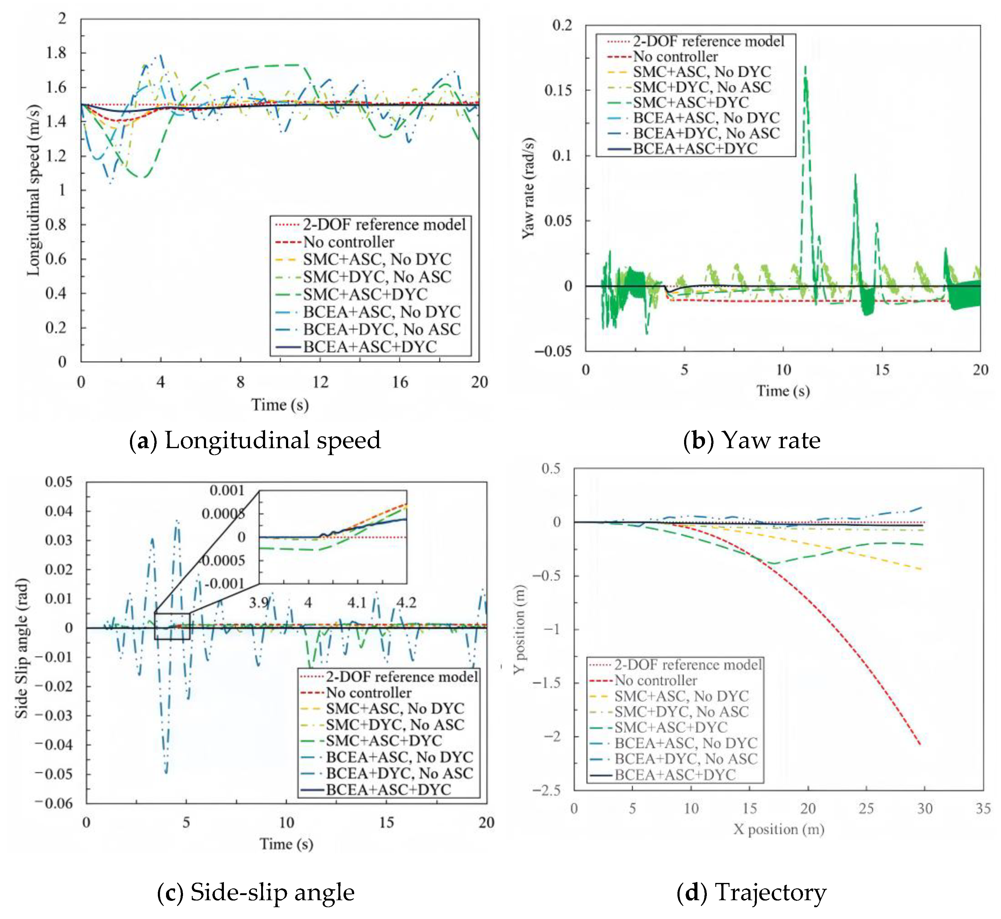
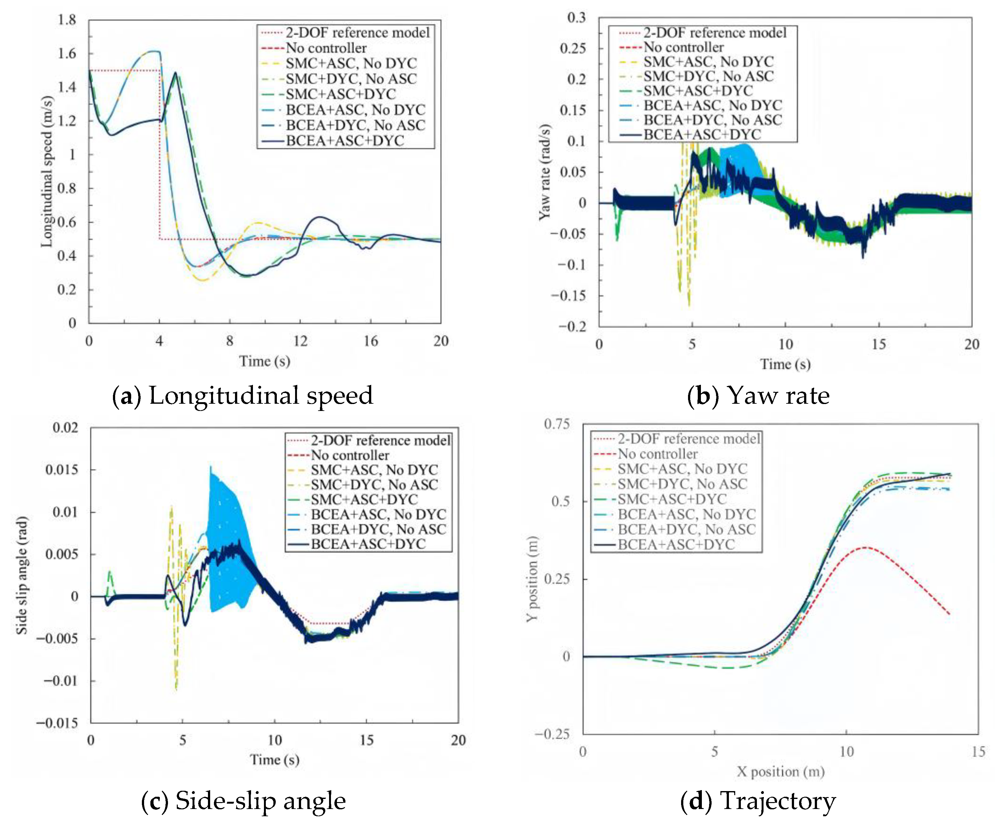
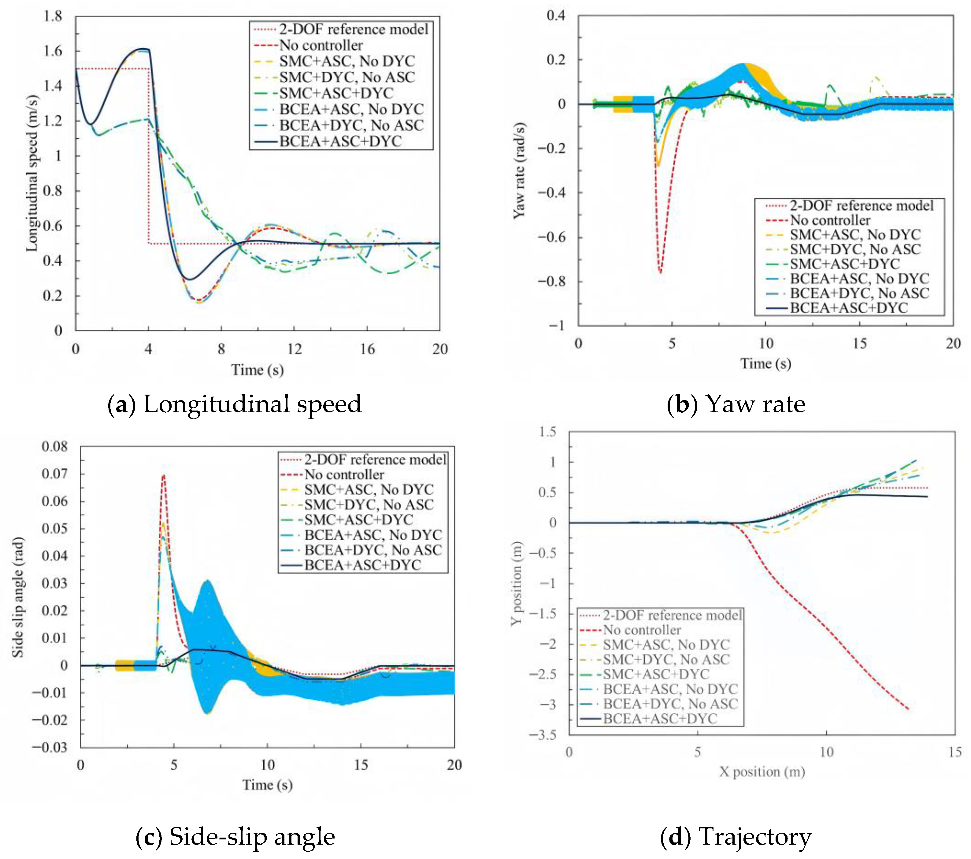
The first test case evaluates the vehicle stability during straight-line motion at a constant speed. Figure 15 and Figure 16 illustrate the longitudinal speed, yaw rate, side-slip angle, and driving trajectory under two specific failure conditions. These include LF tire blowout and LF+RR tire blowout.

As shown in Figure 15 and Figure 16, the proposed “BCEA+ASC+DYC” controller outperforms other BCEA-based RL controllers and SMC-based controllers for both vehicles with “LF” and with “LF+RR” for the straight-line scenario.

To quantify the control performance, the root mean square error (RMSE) is adopted as the evaluation metric. The RMSEs for longitudinal speed ($RMS{E}_u$) and trajectory tracking ($RMS{E}_{tra}$) are defined as

$$\{\begin{array}{c}RMS{E}_u=\sqrt{{\displaystyle \frac{{{\displaystyle \sum }}_{i=1}^N{\left(u_i-u_{xref|i}\right)}^2}{N}}}\\ RMS{E}_{tra}=\sqrt{{\displaystyle \frac{{{\displaystyle \sum }}_{i=1}^N{\left(x_i-x_{ref|i}\right)}^2+{\left(y_i-y_{ref|i}\right)}^2}{N}}}\end{array}$$

(50)

The comparative results are listed in

Table 5. Performance comparison for straight-line scenario ($RMS{E}_u$s and $RMS{E}_{tra}$s).

Blowout Scenario	Controller	$\mathit{R}\mathit{M}\mathit{S}{\mathit{E}}_{\mathit{u}}$	Improvement of ${\mathit{R}\mathit{M}\mathit{S}\mathit{E}}_{\mathit{u}}$ Compared to “No Controller”	${\mathit{R}\mathit{M}\mathit{S}\mathit{E}}_{\mathit{t}\mathit{r}\mathit{a}}$	Improvement of ${\mathit{R}\mathit{M}\mathit{S}\mathit{E}}_{\mathit{t}\mathit{r}\mathit{a}}$ Compared to “No Controller”
LF	No controller	0.033	N/A	0.875	N/A
	SMC+ASC, No DYC	0.042	−27.27%	0.325	62.86%
	SMC+DYC, No ASC	0.121	−266.67%	0.318	63.66%
	SMC+ASC+DYC	0.185	−460.61%	0.575	34.29%
	BCEA+ASC, No DYC	0.081	−145.45%	0.281	67.89%
	BCEA+DYC, No ASC	0.146	−342.42%	0.341	61.03%
	BCEA+ASC+DYC	0.016	51.52%	0.175	80.00%
LF + RR	No controller	0.085	N/A	5.868	N/A
	SMC+ASC, No DYC	0.084	1.18%	0.485	91.73%
	SMC+DYC, No ASC	0.196	−130.59%	10.555	−40.15%
	SMC+ASC+DYC	0.082	3.53%	0.483	93.59%
	BCEA+ASC, No DYC	0.191	−124.71%	2.411	67.99%
	BCEA+DYC, No ASC	0.098	−15.29%	1.125	85.06%
	BCEA+ASC+DYC	0.039	54.12%	0.438	94.18%

.

Table 5 shows that the integrated “BCEA+ASC+DYC” achieves the optimal control performance. Under the “LF” blowout condition, longitudinal speed tracking accuracy improves by 51.52%, and trajectory accuracy improves by 80%. Under the “LF+RR” blowout condition, these improvements reach 54.12% and 94.18%, respectively. This confirms the superior performance of the proposed method in maintaining stability under sudden failure.

(b)

Single lane change (SLC) scenario

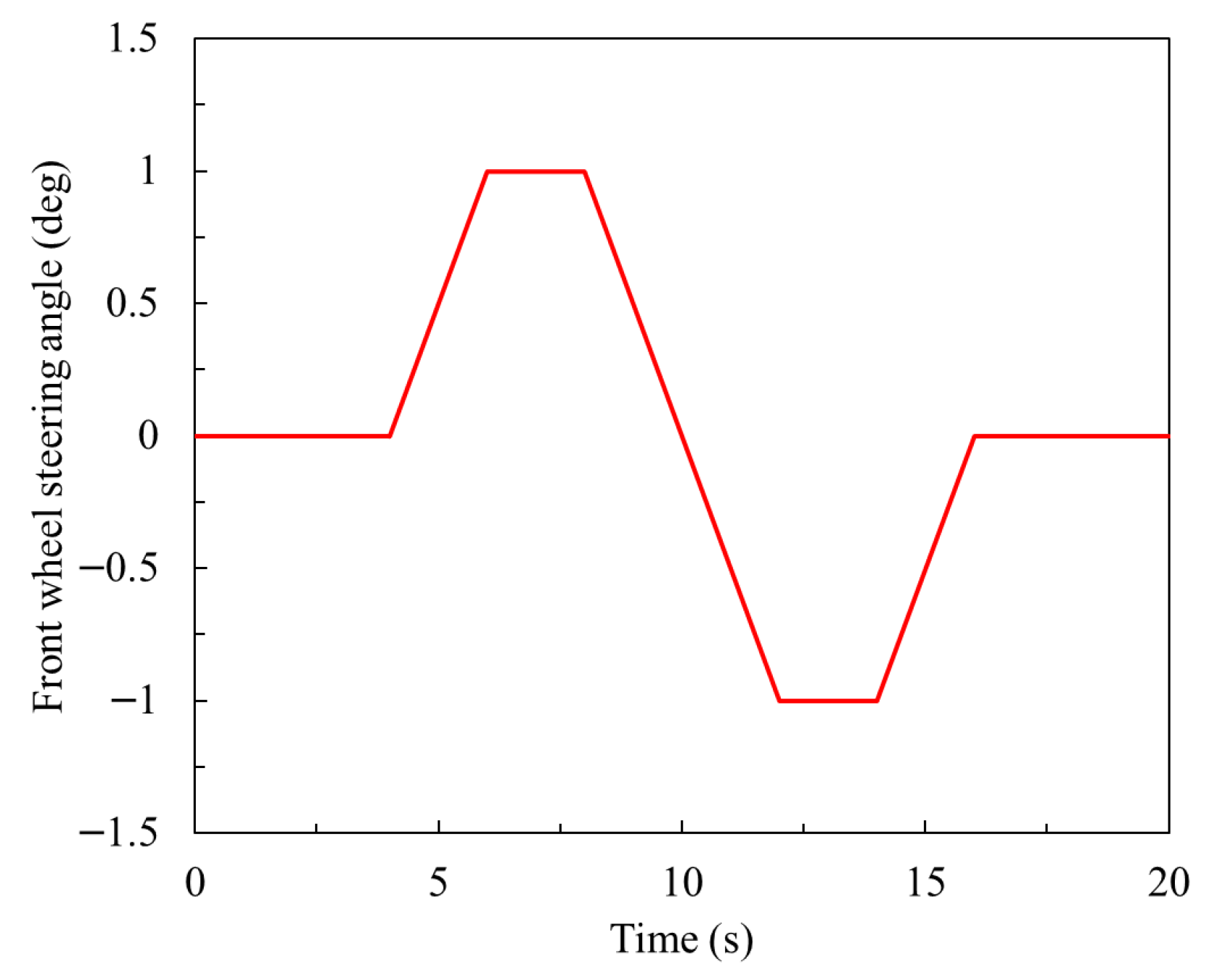
SLC maneuver represents a critical dynamic scenario. In this test, the vehicle velocity decelerates from 1.5 m/s to 0.3 m/s (kinematically equivalent to a full-scale deceleration from 90 km/h to 18 km/h). The input steering input profile is illustrated in Figure 17.

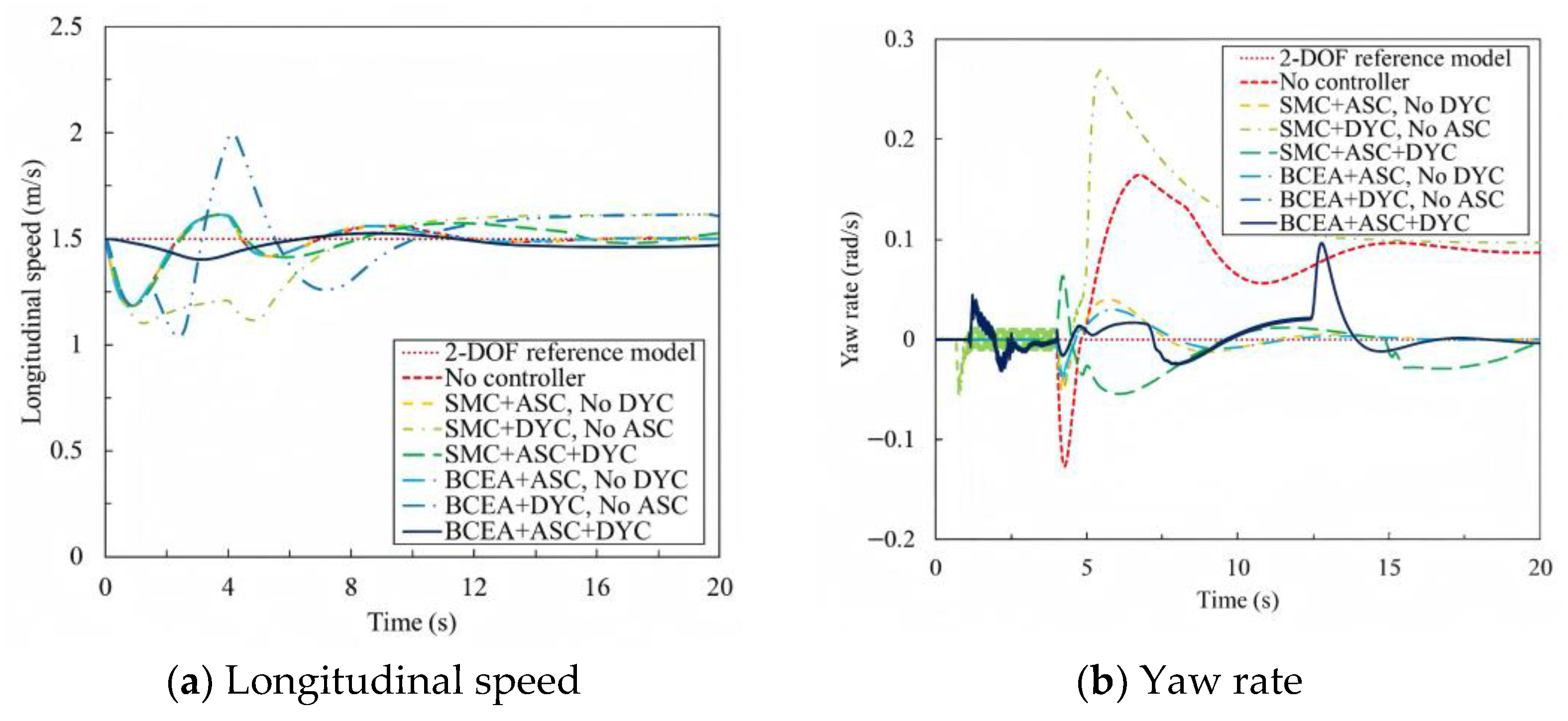
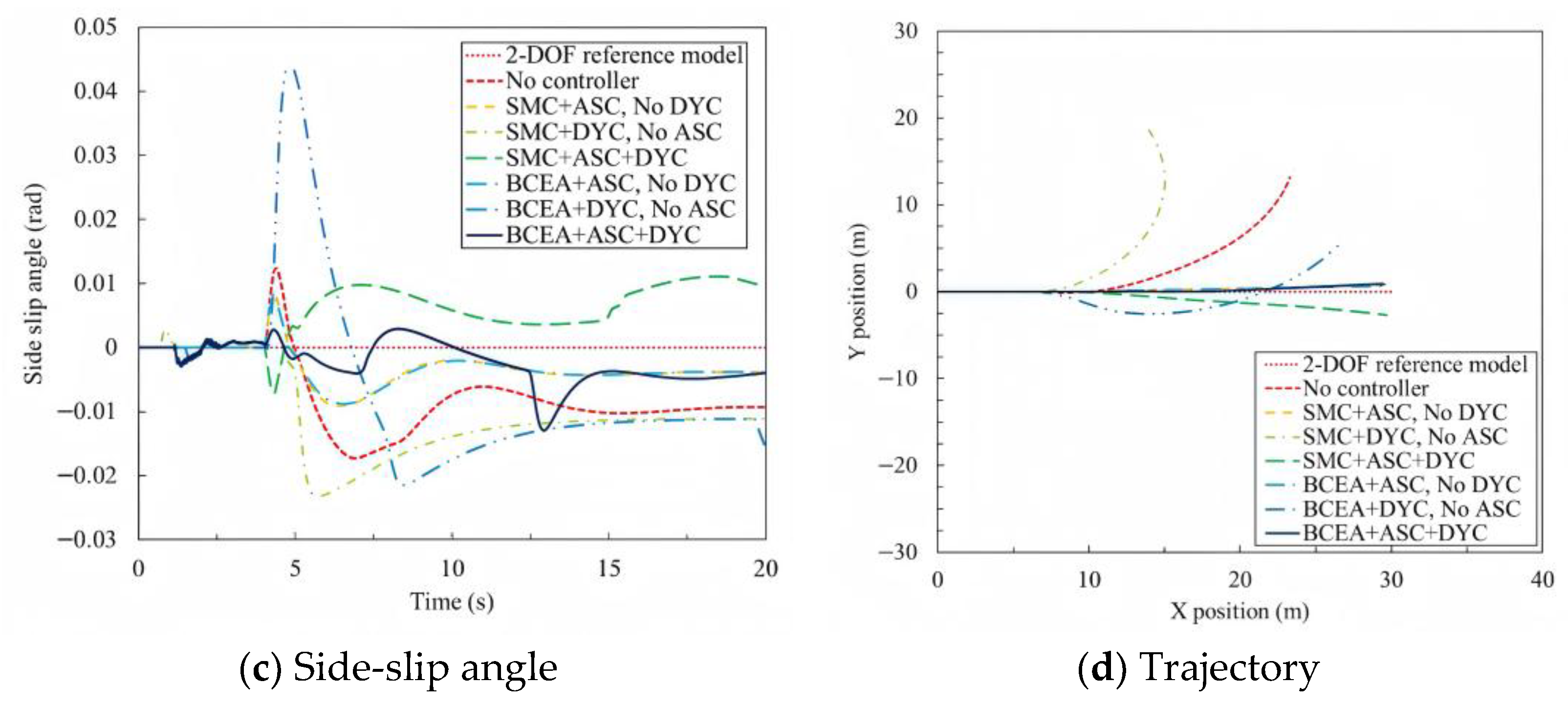
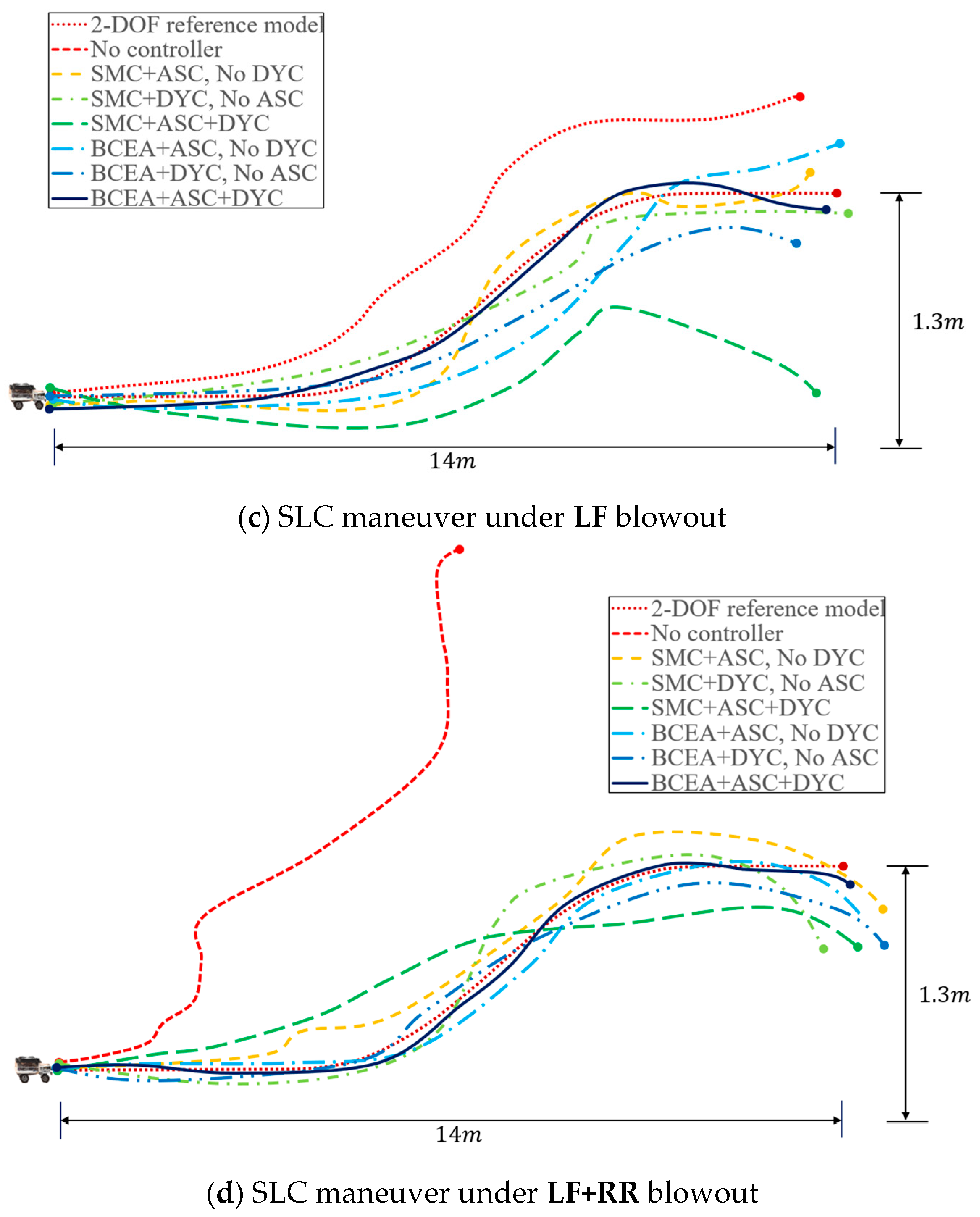
Figure 18 and Figure 19 display the simulation results for the “LF” and “LF+RR” blowout conditions during the SLC scenario.

As shown in Figure 18 and Figure 19, the proposed “BCEA+ASC+DYC” controller outperforms other BCEA-based RL controllers and SMC-based controllers for both vehicles with “LF” and with “LF+RR” for the SLC scenario. The RMSEs for the SLC scenario are listed in

Table 6. Performance comparison for SLC scenario ($RMS{E}_u$ and $RMS{E}_{tra}$).

Blowout Scenario	Controller	$\mathit{R}\mathit{M}\mathit{S}{\mathit{E}}_{\mathit{u}}$	Improvement of ${\mathit{R}\mathit{M}\mathit{S}\mathit{E}}_{\mathit{u}}$ Compared to “No Controller”	${\mathit{R}\mathit{M}\mathit{S}\mathit{E}}_{\mathit{t}\mathit{r}\mathit{a}}$	Improvement of ${\mathit{R}\mathit{M}\mathit{S}\mathit{E}}_{\mathit{t}\mathit{r}\mathit{a}}$ Compared to “No Controller”
LF	No controller	0.366	N/A	0.261	N/A
	SMC+ASC, No DYC	0.181	50.55%	0.201	22.99%
	SMC+DYC, No ASC	0.173	52.73%	0.318	−21.84%
	SMC+ASC+DYC	0.301	17.76%	0.426	−63.22%
	BCEA+ASC, No DYC	0.167	54.37%	0.183	29.89%
	BCEA+DYC, No ASC	0.153	58.20%	0.186	28.74%
	BCEA+ASC+DYC	0.101	72.40%	0.147	43.68%
LF + RR	No control	0.213	N/A	2.058	N/A
	SMC+ASC, No DYC	0.203	4.69%	0.317	84.60%
	SMC+DYC, No ASC	0.246	−15.49%	0.468	77.26%
	SMC+ASC+DYC	0.262	−23.00%	0.489	76.24%
	BCEA+ASC, No DYC	0.197	7.51%	0.278	86.49%
	BCEA+DYC, No ASC	0.269	−26.29%	0.539	73.81%
	BCEA+ASC+DYC	0.148	30.52%	0.199	90.33%

.

In the SLC scenario, the collaborative “BCEA+ASC+DYC” controller significantly outperforms conventional SMC method. Under the “LF” blowout condition, improvements of 72.40% in speed tracking and 43.68% in trajectory tracking are observed. Under the “LF+RR” blowout condition, the maximum improvement in longitudinal speed tracking and trajectory tracking are 30.52% and 90.33%, respectively, as compared with no controller, demonstrating enhanced robustness.

4.4. Scaled Prototype Tests

It is necessary to validate the proposed control strategies through a physical test on the prototype. The experiments utilize the high-precision gyroscope within the Sense HAT module to record the real-time trajectory of the vehicle. Due to current experimental constraints, installing a tire blowout simulation device on the prototype vehicle is not feasible. Such a device involves complex mechanical structures, electro-pneumatic and hydraulic systems, presenting significant challenges in design, manufacturing, and calibration. Consequently, the prototype tests are conducted exclusively with tires in a pre-set blown-out state.

The prototype road tests were conducted in a big room. The test area covers approximately 200 m². The friction coefficient of the road surface is 0.27.

The total delay of the system is about 200 ms. This delay comes mainly from signal transmission, execution of the BCEA algorithm and response of the motor command. The value falls within the typical delay range of the drive-by-wire chassis system and does not exceed the requirements of the maximum delay that are recognized by the automotive industry [68,69]. The sampling period of the tire pressure sensor is set to 40 ms.

The theoretical efficiency for achieving a real-time safety margin is guaranteed through three aspects. First, the controller is trained by a single-layer neural network that has a fast computation speed. The measured computation delay accounts for only 5 percent of the total delay. Second, the control strategy is effective for both normal driving and tire blowout conditions. The proposed controller always provides collaborative active steering and direct yaw moment control, which ensures continuous and reliable control responses in both normal and tire blowout situations. Finally, scaled prototype road tests verify that the overall system delay is only 200 milliseconds, which is significantly lower than the critical requirement of 500 milliseconds in the automotive industry. This demonstrates that the theoretical effectiveness is sufficient, thereby ensuring an adequate real-time safety margin.

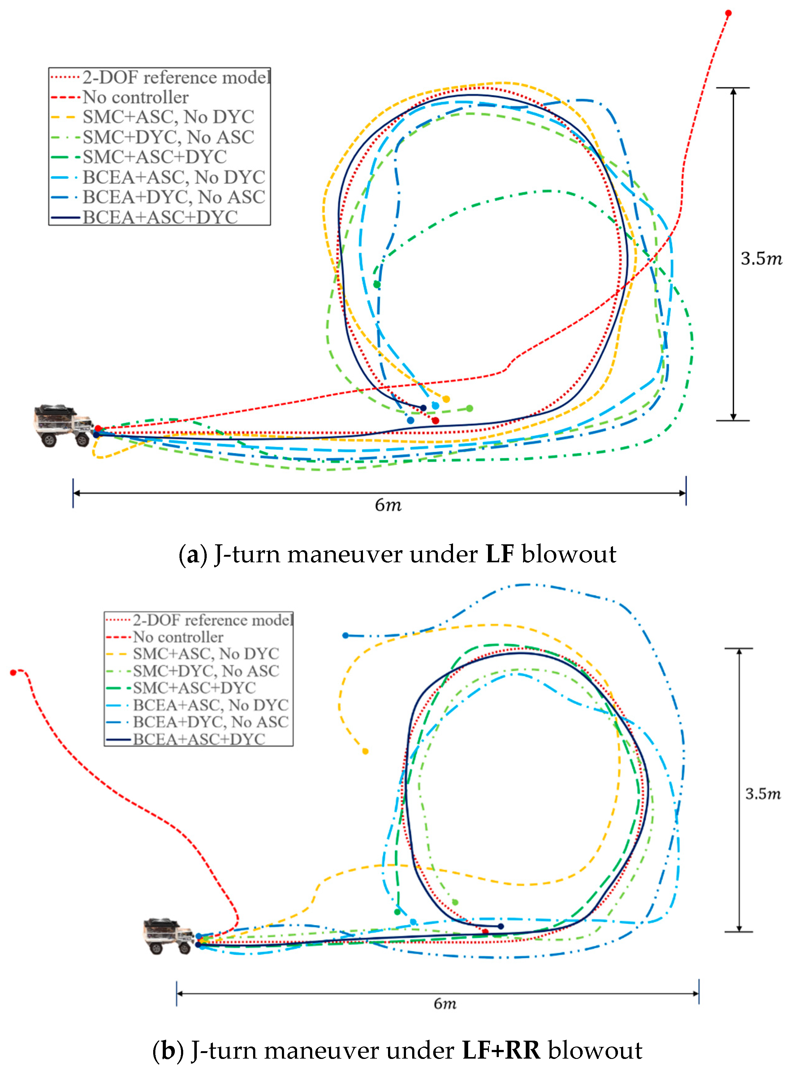
Two specific extreme conditions are selected for evaluation, including a “LF” blowout condition and a “LF+RR” blowout condition. The tire blowouts are applied prior to the tests, as shown in Figure 13, because instant tire failure cannot be achieved during actual road tests. These faults are tested under two dynamic maneuvers: (a) J-turning and (b) SLC, which represent typical driving scenarios where a vehicle must be guided to a maintenance area for repair. The comparative trajectory results for these tests are presented in Figure 20.

As shown in Figure 20, the proposed “BCEA+ASC+DYC” controller outperforms the other BCEA-based and SMC-based controllers in trajectory tracking for both the J-turning and SLC maneuvers.

The quantitative performance is evaluated using the RMSE of the trajectory $RMS{E}_{tra}$ as shown in Equation (50). The results for the J-turning and SLC scenarios are listed in

Table 7. Experimental results for J-turning scenario ($RMS{E}_{tra}$).

Blowout Scenario	Controller	$\mathit{R}\mathit{M}\mathit{S}{\mathit{E}}_{\mathit{t}\mathit{r}\mathit{a}}$	Improvement of ${\mathit{R}\mathit{M}\mathit{S}\mathit{E}}_{\mathit{t}\mathit{r}\mathit{a}}$ Compared to “No Controller”
LF	No controller	9.275	N/A
	SMC+ASC, No DYC	0.459	95.05%
	SMC+DYC, No ASC	0.716	92.29%
	SMC+ASC+DYC	2.768	70.16%
	BCEA+ASC, No DYC	0.473	94.91%
	BCEA+DYC, No ASC	0.581	93.74%
	BCEA+ASC+DYC	0.324	96.51%
LF and RR	No controller	6.498	N/A
	SMC+ASC, No DYC	2.598	60.01%
	SMC+DYC, No ASC	0.499	92.32%
	SMC+ASC+DYC	1.079	83.39%
	BCEA+ASC, No DYC	0.859	86.79%
	BCEA+DYC, No ASC	3.953	39.17%
	BCEA+ASC+DYC	0.209	96.78%

and

Table 8. Experimental results for SLC scenario ($RMS{E}_{tra}$).

Blowout Scenario	Controller	$\mathit{R}\mathit{M}\mathit{S}{\mathit{E}}_{\mathit{t}\mathit{r}\mathit{a}}$	Improvement of ${\mathit{R}\mathit{M}\mathit{S}\mathit{E}}_{\mathit{t}\mathit{r}\mathit{a}}$ Compared to “No Controller”
LF	No controller	0.918	N/A
	SMC+ASC, No DYC	0.521	43.32%
	SMC+DYC, No ASC	0.239	74.04%
	SMC+ASC+DYC	1.381	−50.43%
	BCEA+ASC, No DYC	0.334	63.66%
	BCEA+DYC, No ASC	0.791	13.87%
	BCEA+ASC+DYC	0.223	75.65%
LF and RR	No controller	7.215	N/A
	SMC+ASC, No DYC	0.759	89.48%
	SMC+DYC, No ASC	0.662	90.83%
	SMC+ASC+DYC	0.616	91.46%
	BCEA+ASC, No DYC	0.745	89.67%
	BCEA+DYC, No ASC	0.933	87.06%
	BCEA+ASC+DYC	0.169	97.67%

.

In the J-turning scenarios, the proposed “BCEA+ASC+DYC” controller demonstrates superior performance compared to all other controllers. As compared with no controller, the proposed controller achieves trajectory tracking improvements of 96.51% under the “LF” blowout condition and 96.78% under the extreme “LF+RR” blowout condition, respectively.

Similarly, in the SLC scenarios, the controller significantly enhances vehicle stability. Performance gains of 75.65% and 97.67%, as compared with no controller, are recorded for the “LF” and “LF+RR” blowout conditions, respectively. These consistent results confirm the adaptability and effectiveness of the proposed control strategy in real-world environments.

4.5. Discussion

The proposed controller demonstrates superior performance across all tested conditions. Compared to the uncontrolled case, the longitudinal speed tracking accuracy has improved significantly, with gains ranging from 27.38% to 80.25% depending on the specific tire blowout scenarios. Similarly, the trajectory tracking accuracy shows substantial enhancements, ranging from 68.9% to 94.18%. This indicates that the “BCEA+ASC+DYC” controller can swiftly stabilize the vehicle and correct its heading immediately after tire blowouts.

The robustness of the system is particularly evident in the most challenging scenarios: the single “LF” blowout and the diagonal “LF+RR” blowout. In the straight-line driving scenario, the controller improves the trajectory tracking by 43.68% for “LF” and 90.33% for “LF+RR”. In the J-turning scenarios, the performance is improved by 96.51% for “LF” and 96.78% for “LF+RR”. In the SLC scenarios, the improvements of 75.65% and 97.67% are recorded. These consistent results under extreme conditions strongly support the practical engineering applicability of the BCEA algorithm.

5. Conclusions

Tire blowouts are hazardous faults that traditional steering controllers often fail to manage effectively. While ASC and DYC offers a solution, the strong coupling between these systems makes controller design challenging. To address this challenge, this study introduces an adaptive controller named BCEA based on RL.

The BCEA controller offers a simpler design architecture and superior robustness compared to traditional methods. Furthermore, it achieves significantly faster training speed, improving the training efficiency by over 80% compared to traditional DDPG. Both simulation and scaled prototype tests verify the ability of controller to maintain vehicle stability during high-speed blowouts

Despite these promising results, this study has certain limitations. In this study, a simplified suspension model is used in the prototype, and road tests are limited to a few specific conditions. Moreover, the scaled prototype introduces practical errors, including sensor zero-offset accumulative error and time delays. Additionally, the current speed estimation assumes “no wheel slip”, which decreases in accuracy during acceleration or on low-friction surfaces. It is important to note that this study focuses solely on the impact of blown-out tire on vehicle dynamic stability. While real-world driver reactions (such as sudden steering or braking) are critical elements of road safety that can exacerbate dangerous conditions, modeling of human driver behavior is beyond the scope of this paper and is not considered in the current control strategy. In addition, this study only considers the rapid loss of tire pressure. Tire explosion conditions are not considered in this study. Finally, offline training may not fully capture the stochastic nature of real-world driving environments.

Future research will focus on several key areas. First, current hardware will be updated including higher-precision sensors and a more advanced vehicle chassis. Furthermore, algorithm refinements will be investigated considering adaptive control errors to further fine-tune the performance. In addition, the training efficiency can be enhanced further with other methods, such as utilizing more efficient meta-heuristic methods. Future work will involve the development and installation of a controllable tire blowout actuator on the experimental prototype. This actuator will be designed to emulate sudden tire pressure decompression scenarios under real vehicle testing conditions. Subsequently, a remote-control test platform with a first-person view will be established. This platform will serve to evaluate the influence of human driver reactions on the control performance. Tire explosion conditions will also be considered in the future. Finally, a full-size vehicle platform will be constructed to validate the effectiveness of the proposed algorithm in real-world settings and to investigate the impact of environmental time delays on control performance. Ultimately, this study establishes a foundation for robust vehicle stability under critical failure modes, directly enhancing road safety and reducing the potential for economic losses and human injuries.