Abstract
In order to determine thermally safe driving parameters of ignition coils for hydrogen internal combustion engines (ICE), a reliable estimation of internal power losses is essential. These losses include resistive winding losses, magnetic core losses due to hysteresis and eddy currents, dielectric losses in the insulation, and electronic switching losses. Direct experimental assessment is difficult because the components are inaccessible, while conventional computer-aided engineering (CAE) approaches face challenges such as the need for accurate input data, the need for detailed 3D models, long computation times, and uncertainties in loss prediction for complex structures. To address these limitations, we propose an artificial intelligence (AI)-based framework for estimating internal losses from external temperature measurements. The method relies on an artificial neural network (ANN), trained to capture the relationship between external coil temperatures and internal power losses. The trained model is then employed within an optimization process to identify losses corresponding to experimental temperature values. Validation is performed by introducing the identified power losses into a CAE thermal model to compare predicted and experimental temperatures. The results show excellent agreement, with errors below 3% across the −30 °C to 125 °C range. This demonstrates that the proposed hybrid ANN–CAE approach achieves high accuracy while reducing experimental effort and computational demand. Furthermore, the methodology allows for a straightforward determination of the coil safe operating area (SOA). Starting from estimates derived from fitted linear trends, the SOA limits can be efficiently refined through iterative verification with the CAE model. Overall, the ANN–CAE framework provides a robust and practical tool to accelerate thermal analysis and support coil development for hydrogen ICE applications.
1. Introduction
The shift towards sustainable transportation represents a critical and multifaceted challenge, driven primarily by the urgent need to combat climate change and lessen reliance on fossil energy sources [1,2,3]. Internal combustion engines (ICEs), which currently underpin the global transport sector, require significant redesign and operational adjustments to effectively integrate carbon-neutral fuels [4,5].
Hydrogen (H2) is a leading candidate among these alternative fuels owing to its high energy density, zero direct CO2 emissions during combustion, and the possibility of being produced via renewable energy pathways [6,7,8]. It can be utilized in ICEs as dedicated fuel [9] or in combination with traditional fuels through bi-fuel [10] or dual-fuel [11] systems in order to improve thermal efficiency and decrease pollutant emissions [12]. Hydrogen’s fast flame speed and wide flammability range enable lean combustion [13,14,15], greatly reducing carbon-based emissions like hydrocarbons and carbon monoxide while improving brake thermal efficiency beyond 50% [16,17,18]. Nonetheless, H2 combustion introduces unique challenges due to its high reactivity and low ignition energy [19,20], necessitating precise control of combustion timing to prevent problems such as backfire [21], misfire [22], pre-ignition [23], knocking [24], and elevated NOₓ emissions [25]. Notably, backfire can trigger knocking, risking damage to pistons and cylinders [26].
Therefore, the necessity of reliable components becomes mandatory to effectively develop and deploy H2-ICE. Previous works [27,28] showed the crucial role of diagnostic feedback integrated into the ignition coil when operating with a H2 engine. Correlations between coil diagnostic signal characteristics and in-cylinder pressure were examined to identify the presence of abnormal combustion, misfire, and good combustion. However, incorporating electronics directly into the coil further tightens the thermal limitations. Hence, a precise and reliable definition of the safe operating area (SOA) for these components is crucial.
In particular, the thermal management of electromechanical components plays a critical role in the development of reliable and long-lasting systems for the automotive industry [29,30]. This is particularly true for devices subjected to high-power densities or operating in thermally demanding environments, such as for ignition coils used in gasoline or, in particular, hydrogen internal combustion engines [27,31,32]. When such components also integrate electronic circuits, thermal design becomes even more critical, as these elements often impose tighter temperature constraints due to their limited thermal tolerance [33,34]. Consequently, the ignition systems must evolve to address the increased thermal, mechanical, and electrical demands inherent to hydrogen use [35,36]. Internal power losses, stemming from electromagnetic and resistive effects, are critical in determining coil temperature and lifespan: exceeding certain thermal thresholds may result in shutdown or damage to the integrated electronics as well as degradation of the windings. However, accurately quantifying these losses is challenging due to the inaccessibility of internal components, the difficulty of isolating sensor measurements from external thermal influences during operation, and the inability to discern the contribution of each internal component [37,38]. In addition to being physically inaccessible, direct measurements within internal coil components can also interfere with the normal operation of the system itself [39]. The integration of sensors in regions such as the magnetic core or internal windings may introduce local thermal or electromagnetic disturbances, altering the distribution of losses and compromising the reliability of the acquired data [40,41]. These constraints make it difficult to obtain representative and non-intrusive internal measurements, thereby limiting the effectiveness of conventional validation strategies and increasing reliance on indirect or simulated data for loss estimation [42,43].
In the case of ignition coils, traditional methods exclusively relying on computer-aided engineering (CAE) models are commonly employed to calculate internal power losses and predict thermal behavior [44,45]. CAE models typically rely on numerical techniques such as finite element analysis (FEA) to simulate the physical behavior of components under defined boundary conditions [46,47]. These tools are employed to model the complex multi-physics phenomena that govern the coil’s thermal behavior, including electromagnetic interactions, electronic circuit dynamics, and heat transfer mechanisms [48,49]. Specifically, a CAE architecture involving the electromagnetic, electronic circuit, and thermal domains allows for the calculation of power losses—concerning primary and secondary windings, magnetic core, dielectric bodies, and electronic components—and provides the spatial distribution of temperatures within the coil, enabling us to accurately define the SOA of the component [50,51,52].
However, this approach presents several limitations. Its effectiveness strongly relies on the availability of accurate input data (e.g., B-H curves, material properties, and boundary conditions), which are not always accessible or measurable with the required precision. Moreover, it requires the development of detailed 3D models, which are often complex, time-consuming, and computationally expensive, particularly in multi-physics simulations. Additionally, a reliable calculation of losses for all the loss sources is not always possible because of the geometric complexity and the difficulty in modeling components such as electronics and dielectric materials [53,54,55].
The growing integration of artificial intelligence (AI) and machine learning (ML), especially through artificial neural networks (ANNs), is proving to be increasingly valuable in the study and optimization of ignition coils [27,28]. Thanks to their ability to process external measurements quickly and accurately, these technologies can serve as effective support tools alongside conventional CAE-based methods, contributing to shorter development times, reduced computational load, and improved design efficiency [56,57,58]. Patil et al. [59] present a study that explores how AI, particularly through Altair’s Physics AI tool, can significantly enhance CAE simulations in the automotive industry. Focusing on the A-pillar trim of a vehicle, the authors demonstrate that AI models trained on historical simulation data can predict stress, displacement, and thermal behavior with high accuracy, achieving confidence scores of up to 99.85%. These predictions dramatically reduce simulation time (by up to 30%) and development costs. The results highlight AI’s potential to complement traditional CAE methods, enabling faster, more efficient, and reliable design processes. Winarno et al. [60] investigate the use of genetic algorithms (GA) for optimizing the geometric configuration of magnetic coils, focusing on parameters such as winding number, layer count, and coil dimensions. Although not limited to ignition coils, the study presents a methodology applicable to coil-based components in automotive systems. The GA successfully identifies coil configurations that improve magnetic field strength and uniformity while minimizing energy loss and material usage. The results highlight the potential of genetic algorithms as an efficient and adaptive design optimization tool for electromagnetic components in automotive applications. Qin et al. [61] propose a methodology to reduce the electromagnetic interference (EMI) emitted by automotive ignition systems using an improved micro-genetic algorithm (I-MGA). The goal of the study is to optimize the structural and operational parameters of the ignition coil to mitigate radiated emissions while maintaining ignition performance. By applying the I-MGA to simulate and tune coil configurations, the study achieved a significant reduction in EMI levels compared to traditional designs, demonstrating the effectiveness of genetic optimization in addressing regulatory and functional challenges in automotive ignition systems.
Present Contribution
This work introduces an innovative AI-based methodology for estimating internal power losses in ignition coils designed for H2 ICEs as well as other fuels (i.e., gasoline, methane, e-fuels, etc.). The core objective is to overcome the above-mentioned limitations of conventional CAE-based approaches. The proposed solution consists of an AI framework comprising two different models. The first one, a feed-forward artificial neural network (FFANN), is trained in order to model the relationship between internal power losses and external temperatures, using data calculated by means of the sole CAE thermal simulations. The second model, a GA, is used as an optimizer, which performs the inverse task: estimating the internal power losses that would produce experimentally observed external temperatures. This strategy allows for a fast and reliable estimation of internal power losses under different operating conditions and ambient temperatures.
The proposed approach is validated by verifying that based on the heat losses estimated by the genetic algorithm, the temperatures predicted by the neural network and those computed by the thermal CAE model are consistent with the target experimental values. Once the model is validated, the estimated results at the evaluated points are used to assess the coil’s SOA limits through a short and simple iterative procedure: the process begins with an initial estimate based on linear trends fitted to known points, followed by validation using the CAE thermal model and refinement if needed. The results show that the proposed framework delivers high prediction accuracy, with errors below 3.1% across a wide range of temperatures (−30 °C to 125 °C) and power levels (1.5 W to 21.4 W), also demonstrating an adequate capability of catching the physics of the system. This confirms the robustness, accuracy, and practicality of the proposed approach and highlights its potential to significantly accelerate and enhance thermal analysis in the H2 coil development process.
This approach shifts the focus from conventional physics-based modeling to a more flexible, data-assisted framework that enhances simulation and prediction capabilities, thus allowing the system to bypass exhaustive trial-and-error procedures; it also provides the foundation for integrating AI into crucial development workflows of ignition systems for ICEs, where traditional methods are limited by data availability, complexity, and computational cost. However, the methodology also introduces new needs, such as high-quality and sufficiently diverse training datasets and the handling of model generalization beyond known operating points, ensuring physical consistency in the absence of direct internal measurements.
2. Materials and Methods
The methodology proposed in this work was based on the integration of four distinct domains: experimental testing, thermal CAE simulation, machine learning, and numerical optimization. This multidisciplinary approach was developed with the aim of estimating the internal power loss distribution within the ignition coil while overcoming the limitations of conventional methods. The approach allowed us to ensure that under given ambient temperatures and operating conditions, the temperatures of the coil’s internal components remained within their limits.
In the following subsections, each domain is described in detail, with a focus on its characteristics and role within the overall methodological workflow. Subsequently, the phases of the methodology are presented.
2.1. Experimental Domain
Experimental testing plays a key role in the development, modeling, and validation of physical systems. In addition to serving as the final verification of a product’s real-world performance, experimental measurements provide boundary conditions for numerical models, enable their validation, and supply data for training or evaluating ML models. In thermal testing, temperature measurements are the primary indicators used to assess the consistency between a CAE model and physical reality. The reliability of testing results depends on the quality of the instrumentation, control of environmental conditions, and repeatability of the procedures.
In this work, experimental testing was used to validate the thermal CAE model and to provide the target values for the optimization algorithm aimed at estimating the internal power loss distribution. Measurements were performed on a sample spark ignition coil, i.e., BAE709-CSMD, developed by Champion Ignition, a Tenneco Group Company (Figure 1), operated under controlled conditions inside a climatic chamber, where it was suspended in air by means of metallic wires. In particular, experimental sampling was carried out at three monitoring locations on the coil surface: resin top (T1), housing side (T2), and housing rear (T3), located below the ignition coil connector. This configuration was chosen to thermally isolate the component from its surroundings, minimizing unwanted heat transfer via conduction.

Figure 1.
BAE709-CSMD spark ignition coil.
The coil operated in still air, within a protective box designed to shield it from chamber ventilation, ensuring natural convection only. Each test consisted of an initial thermal stabilization phase with the coil unpowered, followed by operation under load until thermal equilibrium was reached. The component was driven under various operating conditions, within different ambient temperatures. Coil temperatures were measured using K-type thermocouples placed at specific locations on the outer surface of the component—corresponding to the monitoring points defined in the CAE thermal model—and were monitored and stored by means of a Hioki LR8431-20 data logger. In addition, voltage and current signals for both primary and secondary windings were recorded through a measurement system including a Tektronix MSO46 oscilloscope, two current probes, a low-voltage probe, and a high-voltage probe. The component was powered using a Chroma 62012P-100-50 power supply, a battery (acting as an additional energy source), and a Tektronix AFG1062 function generator. Current and low-voltage probes were placed at the output of the power supply. The experimental scheme is highlighted in Figure 2.
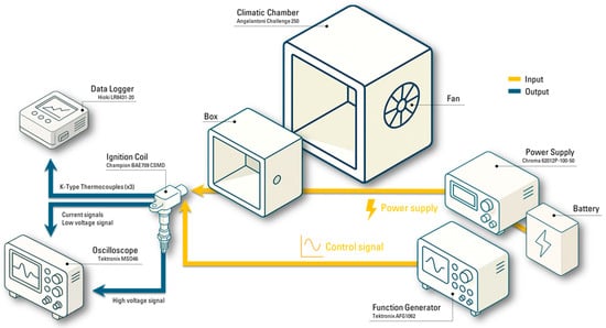
Figure 2.
Experimental setup scheme.
For each test condition, an initial phase was present where the coil was left unpowered inside the chamber at a specified temperature; once the thermal steady-state was reached, the coil was powered with the desired driving and the above-mentioned measurements are taken (start of the test). When the thermal equilibrium was reached again, the final measurements were taken (end of the test). The thermal steady-state condition was assumed once no appreciable changes were observed in the external surface temperatures. Total test durations ranged from two to three hours, depending on the ambient temperature and operating condition.
2.2. Thermal CAE Domain
Thermal CAE simulation is a well-established and widely used method for analyzing and predicting the temperature distribution within engineering components, being particularly valuable when experimental access to internal thermal quantities is limited or unfeasible or when rapid exploration of alternative design scenarios is required. The method is based on the numerical solution—typically using the finite element method (FEM)—of the heat equation, which is expressed, in its classical form, as (Equation (1)):
where
- = material density [kg/m3];
- = specific heat at constant pressure [J/(kg·K)];
- = temperature [K];
- = time [s];
- = thermal conductivity [W/(m·K)];
- = heat generation source [W/m3].
In the case of steady-state analysis, as adopted in this work, the time derivative term becomes zero; thus, the equation simplifies to the following (Equation (2)):
This equation is numerically solved over the three-dimensional solid domain of the component, considering boundary conditions and internal heat generation. This allows it to incorporate all the types of heat transfer mechanisms, conduction, convection, and radiation, and to define spatially distributed heat sources in order to compute the resulting temperature field. The reliability of the results depends on the quality of the geometric modeling and the computational grid, the accuracy of material thermal properties, and the correct definition of boundary conditions and internal heat sources. For this reason, thermal CAE is often combined with experimental data or other numerical models to achieve a realistic and predictive representation of the system’s thermal behavior.
In the proposed methodology, the thermal CAE model (Figure 3) domain played a central role, with a dual purpose: generating the dataset for the FFANN and computing the internal temperatures of the coil under the operating conditions of interest. The model, developed in Ansys Mechanical, was three-dimensional and included the entire geometry of the coil. The windings were represented as homogeneous envelopes, rather than explicitly modeling individual wires, to reduce complexity without affecting the thermal behavior of the system. All the parts were given their materials, characterized by known thermal properties. All the analyses were steady-state, accounting for natural convection and radiative heat exchange with the environment. Internal heat generation must be considered as the effect of power losses arising from resistive, magnetic, dielectric, and electronic effects, whose entity and spatial distribution was the primary focus of this study. Ambient temperature was varied between −30 °C and +125 °C, which represent the extreme ambient working conditions. While the output of the model was the complete temperature field over the whole domain, temperatures were monitored on the outer surfaces in the same points where experimental measurements are available (Figure 3).
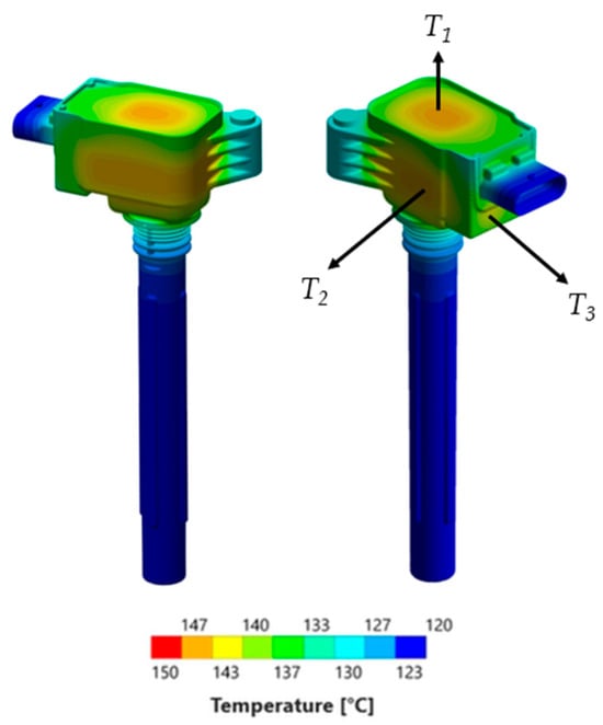
Figure 3.
CAE thermal model representation.
2.3. Machine Learning Domain
ML is a subset of AI that focuses on the development of algorithms capable of learning patterns from data and making predictions or decisions without being explicitly programmed for specific tasks [62]. In engineering applications, ML techniques, particularly neural networks, are increasingly used to approximate complex, nonlinear relationships between input and output variables. These data-driven models offer powerful tools for system identification, behavioral prediction, and optimization, making them well suited for tasks involving large datasets, uncertain dynamics, or inaccessible internal states [63].
In the proposed methodology, a FFANN, trained on data derived from the CAE thermal model, was employed to model the relationships between coil power losses and external temperatures. Each sample in the dataset consisted of five input features, corresponding to the volumetric power losses (in W/mm3) within the main internal components: primary winding, secondary windings, iron core, dielectric bodies, and IGBT (i.e., insulated-gate bipolar transistor). The associated outputs were the steady-state temperatures at three key monitoring locations on the component’s external surface (Figure 3). For each operating condition, the dataset included 600 instances and was randomly shuffled and divided into three subsets: 70% for training, 15% for validation, and 15% for testing.
The FFANN architecture consists of an input layer with five neurons (corresponding to the number of input features), followed by three hidden layers (Figure 4). The number of neurons in each hidden layer is selected through a hyperparametric grid search and may vary depending on the configuration, allowing the model to balance accuracy and generalization. Each hidden layer uses the rectified linear unit (ReLU) as the activation function, which introduces non-linearity between layers and promotes an efficient convergence during training. The output layer contains three neurons corresponding to the predicted surface temperatures.
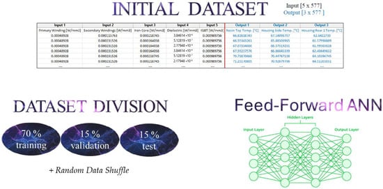
Figure 4.
FFANN setup and dataset division.
Training was performed with a maximum of 100,000 epochs. However, early stopping strategies were employed to terminate the process after 100 consecutive validation iterations with no performance improvement, thus preventing overfitting and reducing computational time. All tasks, encompassing the development, training, and optimization of the model, were carried out within the MATLAB R2024a environment, using a single CPU and 16 GB of RAM.
2.4. Optimization Domain
Optimization is a fundamental aspect of engineering design and analysis, particularly when determining the set of input parameters that best satisfies a given objective function under defined constraints [64]. Among the available strategies, evolutionary algorithms, such as genetic algorithms, have gained prominence for their ability to handle complex, nonlinear, and high-dimensional problems where traditional optimization methods may fall short [65]. Inspired by the mechanisms of natural evolution, GAs explore the solution space by evolving a population of candidate solutions through processes such as selection, crossover, and mutation. Their adaptability and robustness make them especially suitable for inverse problems, where inputs must be inferred based on known outputs [60,66].
In this work, while the FFANN was used to identify the relationship between the internal power losses and the external temperatures of the coil, a GA was employed to solve the inverse problem: the estimation of internal power losses starting from external temperatures measured experimentally. This provided the CAE thermal model with the needed inputs to calculate the temperature distribution for the given operating condition.
As shown previously, the FFANN maps a five-dimensional input vector according to Equation (3):
where each represents an internal volumetric power loss associated with one of the following components: primary winding, secondary windings, iron core, dielectric bodies, and IGBT.
The network returns the predicted surface temperature vector , which is then compared to the experimentally measured reference vector using a cost function (Equation (4)):
where L quantifies the discrepancy between predicted and target temperatures.
The GA model embeds the relations coming from the FFANN within an optimization loop (Figure 5): at each iteration, it generates a population of candidate power loss vectors, evaluates their fitness using the cost function, and applies genetic operations (‘selection’, ‘crossover’, and ‘mutation’) to evolve the population toward the optimum. The process continues until the error between predicted and target temperatures falls below a predefined-costumer acceptability threshold.
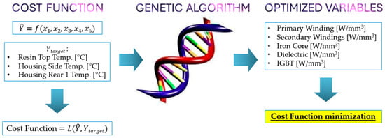
Figure 5.
GA workflow representation.
The genetic algorithm used in this work was configured with a population size of 25 individuals to maintain a diverse pool of candidate solutions. The optimization was run for a maximum of 100 generations, allowing for sufficient iterations for convergence. A crossover fraction of 0.8 was employed, ensuring that 80% of the population participated in recombination at each generation to enhance genetic diversity and facilitate effective exploration of the solution space.
2.5. Methodological Framework
In the first phase (Figure 6, step 1), thermal testing of the coil was conducted across diverse ambient temperatures and operating points by varying the input power, expressed as a combination of the driving parameters, namely charging time, supply voltage, and frequency. At each operating point, steady-state temperatures were measured at three specific locations on the outer surface of the component, as reported in Figure 3. These measurements served as target values for the proposed methodology.
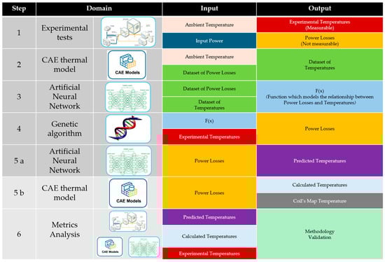
Figure 6.
The phases of the methodology.
In the second phase (Figure 6, step 2), the CAE model was fed with 600 different combinations of internal heat generation on the 5 dissipating parts (primary winding, secondary windings, iron core, dielectric bodies, IGBT), which resulted in as many simulation runs, which were automatically launched in batch. For a given operating condition (i.e., ambient temperature and input power), this allowed us to build a dataset where, for each combination, the 5 dispersions were related to the corresponding temperatures calculated by the model in the 3 above-mentioned points of interest lying on the outer surface of the coil (Figure 3). The power loss combinations were randomly generated by means of a PYTHON 3.11.12 (64 bit) 3.11.12 (64 bit) tool, imposing a specific range constraint for each part, according to the physics of the dispersion (e.g., ohmic heating was expected to be the most relevant contribution). Such block of 600 simulation runs was repeated for every operating condition in order to build the datasets to feed the FFANN for the training, validation, and testing steps.
In the third phase (Figure 6, step 3), all the datasets derived from the thermal CAE model, specifically the input power losses and the corresponding external temperature fields, were used to train the FFANN. In this phase, various instances of internal power losses were provided as input to the FFANN, which was trained to predict the resulting external temperatures at the predefined monitoring points. This model captured the relationship between internal heat generation and external temperatures. The training phase was critical, as it enabled the neural network to generalize the system’s thermal behavior across the different operating conditions tested.
In the fourth phase (Figure 6, step 4), the complex relationship between power losses and external temperatures, as modeled by the FFANN, was passed to the GA optimization algorithm. Starting from the target experimental temperatures, this algorithm exploited such a relationship to iteratively search for the corresponding internal power losses. The optimization was guided by minimizing the error between GA-estimated and target temperatures (as reported in Section 2.4).
In the fifth phase of the process, the GA-derived power losses were used for the inference with the FFANN (Figure 6, step 5a) and as internal heat generation sources in the CAE thermal model (Figure 6, step 5b) for the following reason: if the models were able to match, within an acceptable tolerance, the experimental temperatures under the same ambient temperature and input power conditions, then the whole system was validated.
Once the model was validated, the final phase (Section 4.4) consisted of using the results of the evaluated points to determine the SOA limits through a straightforward iterative procedure: the known points were fitted linearly, and an initial estimate was performed of the limit input and the corresponding power losses, which were supposed to lead the IGBT to its 150 °C limit; the estimated point was then verified through the CAE thermal model in terms of IGBT temperature, and if necessary, the estimation was refined. The resulting SOA curve provided safe and reliable operation limits for ignition coil operation across the full range of thermal conditions.
3. Test Campaign
The experimental campaign investigated the steady-state temperatures at various locations on the surface of the ignition coil, presented in Section 2.1, across different ambient conditions and input power levels. As highlighted in Table 1, the ambient temperatures tested were −30 °C, 0 °C, 30 °C, 60 °C, 90 °C, and 125 °C, ranging from extreme cold to hot environments. For each ambient condition, multiple working points were defined, characterized by different combinations of input power and driving modes (labeled ‘Driving 1’ to ‘Driving 5’). Input power ranged from 1.5 W to 21.4 W, allowing for the study of both low-power and high-power scenarios. The supply voltage was fixed at approximately 14 V, while the charge time and frequency varied, within coil specifications. At a given power input, the driving modes were ordered in increasing charge time, which corresponded to a decrease in driving frequency from Driving 1 to Driving 5.

Table 1.
Working conditions for the tested points.
Temperatures were measured at three locations using thermocouples. These locations captured the heat distribution and identify thermal hotspots. This approach allowed for the evaluation of how different driving strategies, at a given input power, affected the thermal behavior of the component. The measured temperatures will serve as reference targets to be matched by both the CAE thermal model and the neural network, providing a benchmark for validating predictive accuracy under various operating conditions. A total of 33 experimental tests were presented, covering a broad range of realistic working scenarios.
4. Results and Discussion
4.1. Prediction Performance Analysis
To evaluate the reliability and accuracy of the proposed model in replicating the thermal behavior of the ignition coil, the mean absolute error () [67] and the mean absolute percentage error () [68] were adopted as key evaluation metrics.
The standard (Equation (5)) quantifies the average absolute deviation between the predicted values and the corresponding reference values obtained from thermal simulations:
where
- = total number of temperature measurements;
- = temperature;
- = CAE simulations temperatures;
- = AI-predicted temperatures.
In addition, a normalized error metric, the MAPE, is calculated to assess the relative deviation of both the CAE model and ANN predictions from the experimental data. This provides a scale-independent indicator of predictive performance (Equation (6)):
where X stands for either CAE or ANN, depending on whether the comparison is made between experimental data and the thermal simulation or the neural network output, respectively. This dual evaluation enables a consistent assessment of the model against experimental evidence.
Figure 7 shows that the between FFANN-GA predictions and CAE simulation results remains consistently low, below 0.5 °C for the majority of operating points and never exceeding 1.5 °C except for a single case, demonstrating a robust alignment between the two models. Additionally, the values, calculated with respect to the experimental surface temperature measurements, are below 3.1% across all test conditions for both FFANN-GA and CAE models. These error levels fall well within the typical uncertainty range of thermocouple instrumentation (±2.2 °C), confirming the reliability of the model predictions.
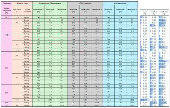
Figure 7.
FFANN and CAE performance analysis.
These good results have been achieved over a wide range of ambient temperatures (from −30 °C to 125 °C) and input power levels (from 1.5 W to over 21.4 W), resulting in a broad range of temperature outputs. This demonstrates the robustness and generalization capability of the FFANN-GA model, which remains accurate even when predicting under diverse operating conditions.
The agreement between predicted and experimentally measured temperatures was quantitatively assessed through the coefficient of determination (R2). As reported in Figure 8, both the ANN and the CAE approaches achieved high correlation with the measured data, confirming the reliability of the proposed hybrid methodology. Specifically, the ANN provided an excellent agreement with the experimental measurements, with R2 values of 0.99932, 0.99930, and 0.99924 for temperatures 1, 2, and 3, respectively. The CAE simulations also yielded consistently high accuracy, with R2 values of 0.98544, 0.98310, and 0.98406 at the same measurement points.
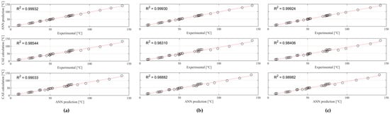
Figure 8.
R2 for (a) T1, (b) T2, and (c) T3, comparing ANN vs. EXP, CAE vs. EXP, and CAE vs. ANN.
In addition, a direct comparison between ANN predictions and CAE results produced R2 values of 0.99033, 0.98882, and 0.98982, further confirming the consistency of the two methods. These findings demonstrate that both components of the proposed hybrid CAE + ANN framework contribute to accurately capturing the thermal behavior of the system, with the ANN offering enhanced precision, while the CAE model ensures physical interpretability.
Furthermore, in addition to the accuracy improvements discussed earlier, the proposed framework offers further advantages over a traditional CAE-only approach. Instead of full multi-domain simulations coupling electromagnetic, electronic, and thermal aspects (each requiring detailed material characterization, complex geometry modeling, and long machine times), the present method relies exclusively on thermal simulations to generate the training data. This avoids cumulative error propagation across domains and provides a more flexible and adaptable workflow.
In terms of effort, building the thermal model required about two man-hours, and 600 simulations for one operating point took roughly 48 h of machine time without human intervention. Once the dataset was available, neural network training took 2 ÷ 4 min, and the optimization converged within 5 ÷ 7 min. By contrast, a multi-domain CAE model typically requires 16 ÷ 24 man-hours to set up, and each simulation run takes 12 ÷ 24 h for a single operating point. These results demonstrate further reductions in both human effort and computational time achieved by the proposed approach.
4.2. Input Power Effects on Performance Prediction
Given the strong agreement between the FFANN-GA model and the CAE predictions, i.e., (Figure 7), as well as the low prediction error of both models, i.e., (Figure 7), it becomes both meaningful and necessary to further investigate if the physics of the system was captured as well. The focus now shifts to a more detailed analysis of the thermal effects induced by variations in input power.
Specifically, in this section, we will focus on a specific ambient condition (0 °C) to investigate how increasing input power impacts heat generation across the different components of the ignition coil. Input power was varied through adjustments in two of the three driving parameters: charging time and excitation frequency, which increase to achieve higher power levels. As a consequence, both Joule losses and frequency-dependent losses intensified with increasing power. The input power ranged from a minimum value of 1.5 W to a value of 18.4 W, which was chosen for applying wide thermal safety margins, and thus, it is expected to be widely within the SOA limits. It is worth highlighting that in order to reach 18.4 W, the charge timing was increased over the max. out specification.
As illustrated in Figure 9, the FFANN-GA model not only captures the overall increase in thermal losses as input power rises but also remarkably succeeds in identifying and reproducing this trend for each individual component within the ignition coil. This level of detail emphasizes the model’s ability to represent thermal phenomena with high precision, demonstrating a deep understanding of the underlying physical behavior. A nearly linear growth in absolute heat generation is observed for all components, with the notable exception of the primary winding. For this component, the trend begins to plateau at an input power of approximately 18.4 W.
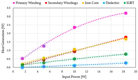
Figure 9.
FFANN-GA prediction of heat generation for primary winding, secondary windings, iron core, dielectric, and IGBT.
This deviation is attributed to the activation of an internal electronic protection mechanism within the ignition coil. Specifically, the driver circuitry imposes a current limit during the charging phase to prevent excessive current buildup that could otherwise lead to overheating or physical damage. This limitation may occur when maximum out specification (MOS) charge time is overpassed. As a result, beyond a certain threshold, further increases in driving parameters do not translate into higher current in the primary winding, effectively capping its Joule losses.
This behavior, correctly predicted by the FFANN-GA model, highlights its robustness not only in capturing smooth, continuous trends but also in detecting the onset of internal protection mechanisms.
4.3. Driving Parameter Effects on Performance Prediction
The next step focuses on a more detailed analysis aimed at exploring the effects induced by variations in the driving parameters while keeping the input power and ambient temperature fixed, i.e., 5 W and 30 °C.
As explained in Section 3 and illustrated in Section 4.1 and Figure 7, to achieve the same input power, the five driving conditions under analysis were arranged in order of increasing charging time, which corresponded to a progressive decrease in excitation frequency from Driving 1 to Driving 5, under constant supply voltage. As detailed in Section 4.2, the increase in charging time leads to more significant Joule losses due to increased current, while frequency-dependent losses, which tend to decrease with lower frequency, play a comparatively minor role. Consequently, the overall rise in thermal losses with increasing driving number (from Driving 1 to Driving 5) is primarily attributed to the dominance of the Joule effect.
This behavior is reflected in the trend of spark energy (Figure 10a), which decreases progressively with increasing driving number. Since spark energy is determined as the residual energy not dissipated through component-level losses (i.e., 100% minus the sum of individual component losses), its inverse correlation with total heat generation is consistent with physical expectations. The heat generation analysis (Figure 10b) also reveals a relatively low and nearly constant contribution from the secondary windings as well as from the iron core, dielectric, and IGBT. In contrast, the primary winding displays a clear increase in its loss share as the driving index increases. This behavior is partly due to the modest variation in temperature observed as the driving mode changes under constant input power. In fact, given the limited thermal gradient across conditions, the network has reduced sensitivity in discerning subtle changes in internal loss distributions. This limitation is further compounded by the system’s topology: all thermal sources are embedded within a single, compact block, making it inherently difficult for the model to spatially resolve the origin of heat contributions, especially considering that it was trained across a wide range of thermal scenarios.
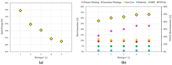
Figure 10.
FFANN-GA prediction of (a) spark energy evolution and (b) heat generation breakdown by individual components and total.
Additionally, as mentioned in the introduction section, since no thermocouples were positioned inside the ignition coil, the model did not receive direct information about internal temperature gradients, further constraining its ability to differentiate localized losses among closely spaced components.
As anticipated, the spark energy trend exhibits a behavior that aligns well with the expected physical interpretation of the system.
4.4. SOA Definition
The SOA is defined by identifying the maximum admissible input power for each ambient temperature condition such that the IGBT temperature does not exceed its thermal limit of 150 °C.
For a given ambient temperature, starting from known experimental input power values and the corresponding IGBT temperatures derived from CAE simulations, a preliminary estimation of the input power required to reach an IGBT temperature of 150 °C was obtained by extrapolation from a linear fitting curve, as depicted in Figure 11a. A linear fitting curve was also employed to estimate the corresponding power losses based on known values (Figure 11b). These extrapolated losses were then used as input to the CAE thermal model to calculate the resulting IGBT temperature. Given that the initial estimation often led to a temperature slightly above or below the target value, the input power was iteratively adjusted around the previously estimated point. This tuning process was continued until the CAE-calculated IGBT temperature closely matched the 150 °C limit, thereby defining the SOA for that specific ambient temperature. This procedure was systematically applied for ambient temperatures of 0 °C, 30 °C, and 60 °C, where a sufficient number of operating points at different input power levels were available. The availability of multiple data points at each of these ambient conditions allowed for a reliable application of the linear fitting method to accurately estimate the input power corresponding to the IGBT thermal limit and to define the SOA with a high degree of confidence. In ambient temperatures for which fewer data points were available, a simplified approach was adopted by applying a linear approximation around the estimated SOA values at 0 °C, 30 °C, and 60 °C.
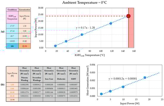
Figure 11.
(a) The linear fitting curve used to determine the input power (red point) corresponding to the IGBT thermal limit (150 °C): example at an ambient temperature of 0 °C. (b) Linear fitting curve used to determine the power losses for the previously estimated input power of 23.9 W.
In these cases, the power losses were assumed to scale proportionally with input power, based on existing reference points, as shown in Figure 12.
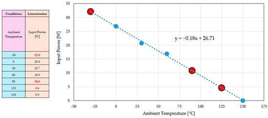
Figure 12.
The linear fitting of SOA input powers as a function of ambient temperature based on known SOA points at IGBTCAE ≅ 150 °C (blue points).
The known SOA values (blue points) are previously determined using the methodology described earlier, involving CAE simulations and the iterative adjustment of input power to reach the IGBT temperature limit.
A linear expression is then used to determine the maximum admissible input power corresponding to each additional ambient temperature (red points), ensuring that the IGBT temperature would not exceed the thermal limit of 150 °C. Once the input power is estimated through this linear fit, the corresponding power losses are determined by applying a direct proportionality with the power losses estimated for the single experimental point available (see Figure 7). These proportionally scaled power losses are then used as input for the CAE thermal simulations to verify the resulting IGBT temperature. If the simulation confirms that the temperature remains at or just below the 150 °C threshold, the point is identified as lying on the SOA boundary; otherwise, the power input is iteratively adjusted according to CAE results. This method allowed for consistent and reliable definition of the SOA across a broader range of ambient conditions.
Figure 13 illustrates the final SOA, including all the estimated points: the resulting fitting curve is a second-order polynomial, which describes the input power limitation across the whole ambient temperature range. Figure 14 highlights all the features concerning the SOA points.
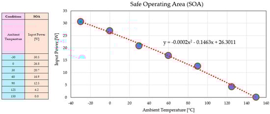
Figure 13.
Input power limits as a function of ambient temperature—SOA definition.
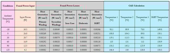
Figure 14.
Final SOA results.
5. Conclusions
This study presents a novel AI-assisted methodology for estimating internal power losses in ignition coils designed for hydrogen internal combustion engines, addressing the limitations of traditional approaches exclusively based on CAE, in terms of computational cost and modeling complexity. By integrating experimental testing, thermal CAE modeling, artificial neural networks, and genetic optimization, the proposed framework enables an accurate estimation of internal heat generation based solely on external temperature measurements, with a limited number of operating conditions that need to be tested.
The methodology demonstrates excellent prediction accuracy across a wide range of ambient temperatures (−30 °C to 125 °C) and input power levels (1.5 W to 21.4 W), confirming the model’s robustness and generalization capabilities. A detailed analysis of the effects of input power variation, for a given ambient temperature, revealed that the FFANN-GA model accurately captures both the overall increase in thermal losses and the component-level trends, including anomalous behavior in the primary winding due to current-limiting protections occurring. Similarly, variations in driving parameters at constant power highlighted the model’s ability to detect physical changes in spark energy.
The study successfully defined the SOA of the ignition coil by identifying the maximum input power at which the IGBT temperature reaches its 150 °C thermal limit. The resulting fitting curve is a second-order polynomial. In general, the described approach allows the CAE thermal model to become predictive in operative conditions that have not been experimentally tested previously since the methodology has been validated both on temperature errors and in terms of capability to capture the underlying physics of the system.
Despite its strengths, the proposed approach shows some limitations in capturing the expected increase in power losses, specifically in cases where surface temperatures remain close to one another, such as when the same input power is applied using different driving conditions. This is due to the reduced thermal gradients available to guide the FFANN and also due to its training on a wide temperature range. From this point of view, future improvements could focus on refining the temperature sampling strategy by increasing the number of thermocouples and on providing improved datasets.
Overall, this work demonstrates the potential of AI as a powerful and efficient tool for product development in advanced automotive applications. By shifting from conventional physics-based modeling to a more flexible, data-assisted framework, it enhances simulation and prediction capabilities, reducing reliance on exhaustive trial-and-error procedures. Furthermore, it lays the foundation for integrating AI into key development workflows for ICE ignition systems, where traditional methods face limitations due to data scarcity, system complexity, and high computational costs.
Author Contributions
Conceptualization, F.R. and M.P.; methodology, F.R. and M.P.; software, F.R. and M.P.; testing, M.P. and F.T.; validation, F.R. and M.P.; formal analysis, F.R. and M.P.; investigation, F.R., M.P., and M.A.; resources, S.P. and M.D.R.; data curation, F.R., M.P., and M.A.; writing—original draft preparation, F.R., M.P., and M.A.; writing—review and editing, F.R., M.P., M.A., S.P., and M.D.R.; visualization, F.R., M.P., and M.A.; supervision, S.P. and M.D.R.; project administration, S.P. and M.D.R. All authors have read and agreed to the published version of the manuscript.
Funding
This study received no external funding.
Data Availability Statement
Dataset available on request from the authors.
Acknowledgments
The ignition coil used for this study was provided by Champion Ignition—Federal-Mogul Powertrain Italy, a Tenneco Group Company.
Conflicts of Interest
Authors Federico Ricci, Mario Picerno, Stefano Papi, Federico Tardini, and Massimo Dal Re were employed by Federal-Mogul Powertrain Italy, a Tenneco Group company, at the time the research was conducted. Author Massimiliano Avana, affiliated with the Department of Engineering at the University of Perugia, declares that he has no commercial or financial relationships that could be construed as a potential conflict of interest.
Abbreviations
The following abbreviations are used in this manuscript:
| AI | artificial intelligence |
| ANN | artificial neural network |
| CAE | computer-aided engineering |
| CFD | computational fluid dynamics |
| CO2 | carbon dioxide |
| CPU | central processing unit |
| EMI | electromagnetic interference |
| FEA | finite element analysis |
| FEM | finite element method |
| FFANN | feed-forward artificial neural network |
| GA | genetic algorithm |
| H2 | hydrogen |
| I-MGA | improved micro-genetic algorithm |
| ICE | internal combustion engine |
| IGBT | insulated-gate bipolar transistor |
| MAE | mean absolute error |
| MAPE | mean absolute percentage error |
| MOS | maximum out specification |
| ML | machine learning |
| NOx | nitrogen oxides |
| R2 | coefficient of determination |
| RAM | random access memory |
| ReLU | rectified linear unit |
| SOA | safe operating area |
References
- Etukudoh, E.A.; Adefemi, A.; Ilojianya, V.I.; Umoh, A.A.; Ibekwe, K.I.; Nwokediegwu, Z.Q.S. A Review of sustainable transportation solutions: Innovations, challenges, and future directions. World J. Adv. Res. Rev. 2024, 21, 1440–1452. [Google Scholar] [CrossRef]
- Wallington, T.J.; Anderson, J.E.; Dolan, R.H.; Winkler, S.L. Vehicle emissions and urban air quality: 60 years of progress. Atmosphere 2022, 13, 650. [Google Scholar] [CrossRef]
- Anika, O.C.; Nnabuife, S.G.; Bello, A.; Okoroafor, E.R.; Kuang, B.; Villa, R. Prospects of low and zero-carbon renewable fuels in 1.5-degree net zero emission actualization by 2050: A critical review. Carbon Capture Sci. Technol. 2022, 5, 100072. [Google Scholar]
- Sinigaglia, T.; Martins, M.E.S.; Siluk, J.C.M. Technological evolution of internal combustion engine vehicles: A patent data analysis. Appl. Energy 2022, 306, 118003. [Google Scholar] [CrossRef]
- Tornatore, C.; Marchitto, L. Advanced technologies for the optimization of internal combustion engines. Appl. Sci. 2021, 11, 10842. [Google Scholar] [CrossRef]
- Baldinelli, A.; Francesconi, M.; Antonelli, M. Hydrogen, E-Fuels, Biofuels: What Is the Most Viable Alternative to Diesel for Heavy-Duty Internal Combustion Engine Vehicles? Energies 2024, 17, 4728. [Google Scholar] [CrossRef]
- Onorati, A.; Payri, R.; Vaglieco, B.; Agarwal, A.; Bae, C.; Bruneaux, G.; Canakci, M.; Gavaises, M.; Gunthner, M.; Hasse, C.; et al. The role of hydrogen for future internal combustion engines. Int. J. Engine Res. 2022, 23, 529–540. [Google Scholar] [CrossRef]
- Shinde, B.J.; Karunamurthy, K. Recent progress in hydrogen fuelled internal combustion engine (H2ICE)—A comprehensive outlook. Mater. Today Proc. 2022, 51, 1568–1579. [Google Scholar] [CrossRef]
- Falfari, S.; Cazzoli, G.; Mariani, V.; Bianchi, G.M. Hydrogen Application as a Fuel in Internal Combustion Engines. Energies 2023, 16, 2545. [Google Scholar] [CrossRef]
- Mohite, A.; Bora, B.J.; Sharma, P.; Medhi, B.J.; Barik, D.; Balasubramanian, D.; Nguyen, V.G.; Js, F.J.; Le, H.C.; Kamalakannan, J.; et al. Maximizing efficiency and environmental benefits of an algae biodiesel-hydrogen dual fuel engine through operational parameter optimization using response surface methodology. Int. J. Hydrogen Energy 2024, 52, 1395–1407. [Google Scholar] [CrossRef]
- Ashkezari, A.Z. Numerical analysis of performance and emissions behavior of a bi-fuel engine with compressed natural gas enriched with hydrogen using variable compression ratio strategy. Int. J. Hydrogen Energy 2022, 47, 10762–10776. [Google Scholar] [CrossRef]
- Aydin, K.; Kutanoglu, R. Effects of hydrogenation of fossil fuels with hydrogen and hydroxy gas on performance and emissions of internal combustion engines. Int. J. Hydrogen Energy 2018, 43, 14047–14058. [Google Scholar] [CrossRef]
- Sementa, P.; Antolini, J.B.d.V.; Tornatore, C.; Catapano, F.; Vaglieco, B.M.; Sánchez, J.J.L. Exploring the potentials of lean-burn hydrogen SI engine compared to methane operation. Int. J. Hydrogen Energy 2022, 47, 25044–25056. [Google Scholar] [CrossRef]
- Avana, M.; Ricci, F.; Papi, S.; Zembi, J.; Battistoni, M.; Grimaldi, C.N. Performance Analysis of Hydrogen Combustion Under Ultra Lean Conditions in a Spark Ignition Research Engine Using a Barrier Discharge Igniter. In SAE Technical Paper 2024-24-0036; SAE International: Warrendale, PA, USA, 2024. [Google Scholar]
- Du, H.; Chai, W.S.; Wei, H.; Zhou, L. Status and challenges for realizing low emission with hydrogen ultra-lean combustion. Int. J. Hydrogen Energy 2024, 57, 1419–1436. [Google Scholar] [CrossRef]
- Shi, C.; Ji, C.; Wang, S.; Yang, J.; Wang, H. Experimental and numerical study of combustion and emissions performance in a hydrogen-enriched Wankel engine at stoichiometric and lean operations. Fuel 2021, 291, 120181. [Google Scholar] [CrossRef]
- Suresh, D.; Porpatham, E. Influence of high compression ratio and hydrogen addition on the performance and emissions of a lean burn spark ignition engine fueled by ethanol-gasoline. Int. J. Hydrogen Energy 2023, 48, 14433–14448. [Google Scholar] [CrossRef]
- Ricci, F.; Zembi, J.; Avana, M.; Grimaldi, C.N.; Battistoni, M.; Papi, S. Analysis of Hydrogen Combustion in a Spark Ignition Research Engine with a Barrier Discharge Igniter. Energies 2024, 17, 1739. [Google Scholar] [CrossRef]
- Kawahara, N.; Azimov, U. Abnormal Combustion in Hydrogen-Fuelled IC Engines. In Hydrogen for Future Thermal Engines; Springer International Publishing: Cham, Switzerland, 2023; pp. 459–482. [Google Scholar]
- Diéguez, P.M.; Urroz, J.; Sáinz, D.; Machin, J.; Arana, M.; Gandía, L. Characterization of combustion anomalies in a hydrogen fueled 1.4 L commercial spark-ignition engine by means of in-cylinder pressure, block-engine vibration, and acoustic measurements. Energy Convers. Manag. 2018, 172, 67–80. [Google Scholar] [CrossRef]
- Marwaha, A.; Subramanian, K.A. Experimental investigation on effect of misfire and postfire on backfire in a hydrogen fuelled automotive spark ignition engine. Int. J. Hydrogen Energy 2023, 48, 24139–24149. [Google Scholar] [CrossRef]
- Hallstadius, P.; Saha, A.; Sridhara, A.; Andersson, Ö. High-Speed Optical Diagnostics of Misfire Limits in a Spark-Ignited Heavy-Duty Hydrogen Engine. In SAE Technical Paper 2025-01-8401; SAE International: Warrendale, PA, USA, 2025. [Google Scholar]
- Distaso, E.; Calò, G.; Amirante, R.; De Palma, P.; Mehl, M.; Pelucchi, M.; Stagni, A.; Tamburrano, P. Linking lubricant oil contamination to pre-ignition events in hydrogen engines—The HyLube mechanism. Fuel 2025, 379, 133041. [Google Scholar] [CrossRef]
- Gao, J.; Yao, A.; Zhang, Y.; Qu, G.; Yao, C.; Zhang, S.; Li, D. Investigation into the relationship between super-knock and misfires in an SI GDI engine. Energies 2021, 14, 2099. [Google Scholar] [CrossRef]
- Pandey, J.K.; Dinesh, M.H.; Kumar, G.N. A comparative study of NOx mitigating techniques EGR and spark delay on combustion and NOx emission of ammonia/hydrogen and hydrogen fuelled SI engine. Energy 2023, 276, 127611. [Google Scholar] [CrossRef]
- Ceschini, L.; Morri, A.; Balducci, E.; Cavina, N.; Rojo, N.; Calogero, L.; Poggio, L. Experimental observations of engine piston damage induced by knocking combustion. Mater. Des. 2017, 114, 312–325. [Google Scholar] [CrossRef]
- Papi, S.; Ricci, F.; Dal Re, M.; Burrows, J.; Daniele, S.; Grimaldi, C.N. Smart Ignition Coil Development for H2 ICE Application. In Proceedings of the 13th Dessau Gas Engine Conference—WTZ Roßlau gGmbH, Dessau-Roßlau, Germany, 15–16 May 2024; pp. 322–335. [Google Scholar]
- Papi, S.; Ricci, F.; Dal Re, M.; Chandelier, M. Smart Ignition Coil Diagnostic System for H2 ICE Combustion Detection. In 6th International Conference on Ignition Systems for SI Engines—7th International Conference on Knocking in SI Engines; Expert Verlag: Berlin, Germany, 2024; pp. 95–124. [Google Scholar]
- Mallik, S.; Ekere, N.; Best, C.; Bhatti, R. Investigation of thermal management materials for automotive electronic control units. Appl. Therm. Eng. 2011, 31, 355–362. [Google Scholar] [CrossRef]
- Johnson, R.W.; Evans, J.L.; Jacobsen, P.; Thompson, J.R.; Christopher, M. The changing automotive environment: High-temperature electronics. IEEE Trans. Electron. Packag. Manuf. 2004, 27, 164–176. [Google Scholar] [CrossRef]
- Ängeby, J.; Johnsson, A.; SEM, J.T.; Zhang, K.; Richter, M.; Ehn, A. Robust ignition and sparkplug wear for H2 SI-ICE. In 6th International Conference on Ignition Systems for SI Engines—7th International Conference on Knocking in SI Engines; Expert Verlag: Berlin, Germany, 2024; p. 81. [Google Scholar]
- Zhang, B.; Rubio, M.; Lam, J.E.T.; Ortiz-Ramirez, A.; Riggs, T.; Hernandez, O.; Chen, Y.; Medchill, C.; Egolfopoulos, F.; Cronin, S.B. Transient plasma enhanced combustion of ultra-lean H2 in an internal combustion engine for reduced NOx emission. Fuel 2025, 381, 133233. [Google Scholar] [CrossRef]
- Szwajca, F.; Wisłocki, K.; Różański, M. Analysis of Energy Transfer in the Ignition System for High-Speed Combustion Engines. Energies 2024, 17, 5091. [Google Scholar] [CrossRef]
- Karimi, K.; Isik, D.; Kong, S.C. Heat Transfer and Thermal Stress Analysis of Ignition Plug During Heating Using Smoothed Particle Hydrodynamics. ASME J. Heat Mass Transf. 2025, 147, 103301. [Google Scholar] [CrossRef]
- Turner, J.W.G. Future technological directions for hydrogen internal combustion engines in transport applications. Appl. Energy Comb. Sci. 2025, 21, 100302. [Google Scholar] [CrossRef]
- Bekdemir, C.; Doosje, E.; Seykens, X. H2-ICE technology options of the present and the near future. In SAE Technical Paper 2022-01-0472; SAE International: Warrendale, PA, USA, 2022. [Google Scholar]
- Arif, A.; Abimanyu, B.; Purwanto, W.; Putra, D.S.; Wagino, W.; Milana, M.; Hidayat, N.; Setiawan, M.Y.; Saputra, H.D. Analysis of primary coil voltage on spark ignition engine using flash cable. BIS Energy Eng. 2025, 2, 225045. [Google Scholar] [CrossRef]
- Monroy Jaramillo, M.; Ramírez Alzate, J.D.; Romero Piedrahita, C.A.; Mejía Hernández, J.C. Experimental and numerical approach to assess the dynamic performance of an inductive ignition system. Int. J. Engine Res. 2024, 25, 1437–1457. [Google Scholar] [CrossRef]
- Vrublevskyi, O.; Wierzbicki, S. Measurement and theoretical analysis of the displacement characteristics of moving components in a solenoid injector in view of wave phenomena. Measurement 2022, 187, 110323. [Google Scholar] [CrossRef]
- Yu, X.; Yu, S.; Yang, Z.; Tan, Q.; Ives, M.; Li, L.; Liu, M.; Zheng, M. Improvement on energy efficiency of the spark ignition system. In SAE Technical Paper 2017-01-0678; SAE International: Warrendale, PA, USA, 2017. [Google Scholar]
- Wang, D.; Wen, Y.; Hu, J.; Zhu, X.; Han, H.; Liu, W. Fault Analysis and Optimization Design of Electronic Ignition System for Fuel Powered Vehicles. In Proceedings of the 2024 International Conference on Electromagnetics in Advanced Applications (ICEAA), Lisboa, Portugal, 2–6 September 2024; pp. 526–530. [Google Scholar]
- Ali, N.M.; Tee, D.L.Y.; Jian, K.H.; Wai, P.T.; Fang, L.S.; Hasan, Z.; Ab Rashid, M.Z.; Razali, S. The Limitations of Present Sensor Technology in Automotive Industry: A Review. J. Telecommun. Electron. Comput. Eng. (JTEC) 2018, 10, 129–134. [Google Scholar]
- Sharma, B.; Thakur, A.; Srivastava, R. The State-of-the-Art Review on the Sensors used in the Automotive Sector. In Proceedings of the 2024 International Conference on Communication, Computer Sciences and Engineering (IC3SE), Gautam Buddha Nagar, India, 9–11 May 2024; pp. 1109–1114. [Google Scholar]
- Kuo, E.Y.; Mehta, P.R.; Prater, G.; Shahhosseini, A.M. Reliability and quality of body concept CAE models for design direction studies. In SAE Technical Paper 2006-01-1617; SAE International: Warrendale, PA, USA, 2006. [Google Scholar]
- Kojima, Y. Mechanical CAE in automotive design. RD Rev. Toyota CRDL 2000, 35, 1. [Google Scholar]
- Louhichi, B.; Abenhaim, G.N.; Tahan, A.S. CAD/CAE integration: Updating the CAD model after a FEM analysis. Int. J. Adv. Manuf. Technol. 2015, 76, 391–400. [Google Scholar] [CrossRef]
- Shuai, L.; Jing, Y.; Bin, L.; Bo, L. Research Based on CAD/CAE/CFD for Collaborative Design of Automotive Engines. In Proceedings of the 2011 Third International Conference on Measuring Technology and Mechatronics Automation, Shanghai, China, 6–7 January 2011; pp. 1044–1047. [Google Scholar]
- Stevenson, R.C.; Palma, R.; Yang, C.S.; Park, S.K.; Mi, C. Comprehensive modeling of automotive ignition systems. SAE Trans. 2007, 116, 1077–1100. [Google Scholar]
- Zhang, L.; Chu, X.; Ding, S.; Zhou, M.; Ni, C.; Wang, X. Surrogate Modeling of Hydrogen-Enriched Combustion Using Autoencoder-Based Dimensionality Reduction. Processes 2025, 13, 1093. [Google Scholar] [CrossRef]
- Wang, Q.; Zhao, Y.; Li, S.; Zhao, Z. Research on energy simulation model for vehicle ignition system. In Proceedings of the 2008 IEEE Vehicle Power and Propulsion Conference, Harbin, China, 3–5 September 2008; pp. 1–5. [Google Scholar]
- Wang, Q.; Zheng, Y.; Yu, J.; Jia, J. Circuit model and parasitic parameter extraction of the spark plug in the ignition system. Turk. J. Electr. Eng. Comput. Sci. 2012, 20, 805–817. [Google Scholar] [CrossRef]
- Paraschiv, M.; Frățilă, G. CAE Approach in Combustion Modeling on a Classic Internal Combustion Engine and Ignition Timing Modeling. In Proceedings of the International Conference of Mechanical Engineering, New Delhi, India, 1–2 September 2022; pp. 293–305. [Google Scholar]
- Tsiolakis, V.; Bensler, H.P. Current CAE trends in the automotive industry. In Computation and Big Data for Transport: Digital Innovations in Surface and Air Transport Systems; Springer: Berlin/Heidelberg, Germany, 2020; pp. 169–179. [Google Scholar]
- Will, J. State of the Art–robustness evaluation in CAE-based virtual prototyping processes of automotive applications. Proc. Optim. Stoch. Days 2007, 4, 1–20. [Google Scholar]
- Kreis, A.; Hirz, M.; Rossbacher, P. CAD-Automation in Automotive Development–Potentials, Limits and Challenges. Comput.-Aided Des. Appl. 2021, 18, 849–863. [Google Scholar] [CrossRef]
- Dubovitskiy, M.A.; Pashaev, S.Y.; Zhukov, A.O. Machine learning based computational electromagnetic methods for intelligence cad/cae application. In Proceedings of the 2021 3rd International Youth Conference on Radio Electronics, Electrical and Power Engineering (REEPE), Moscow, Russia, 11–13 March 2021; pp. 1–6. [Google Scholar]
- Kohar, C.P.; Greve, L.; Eller, T.K.; Connolly, D.S.; Inal, K. A machine learning framework for accelerating the design process using CAE simulations: An application to finite element analysis in structural crashworthiness. Comput. Methods Appl. Mech. Eng. 2021, 385, 114008. [Google Scholar] [CrossRef]
- Ma, Y.; Wang, X.; Dang, K.; Zhou, Y.; Yang, W.; Xie, P. Intelligent recommendation system of the injection molding process parameters based on CAE simulation, process window, and machine learning. Int. J. Adv. Manuf. Technol. 2023, 128, 4703–4716. [Google Scholar] [CrossRef]
- Patil, A.; Sonavane, P. AI-Enhanced CAE Simulations: A Revolutionary Approach to Automotive Design and Engineering. In SAE Technical Paper 2025-01-8241; SAE International: Warrendale, PA, USA, 2025. [Google Scholar]
- Winarno, B.; Paracha, Z.J.; Subkhan, M.F.; Kusumo, R.J.; Lestariningsih, T.; Atmaja, A.P.; Basuki, I. Optimization of magnetic coil construction using genetic algorithm method. J. Phys. Conf. Ser. 2021, 1845, 012008. [Google Scholar] [CrossRef]
- Qin, Y.; Li, B.; Liu, Q.; Xu, X.; Zhai, J. A method for improving radiated emission of automotive spark-ignition system with improved micro-genetic algorithm. In FISITA 2012 World Automotive Congress: Volume 6—Vehicle Electronics Berlin, Heidelberg; Springer: Berlin/Heidelberg, Germany, 2012; Volume 6, pp. 557–564. [Google Scholar]
- Shinde, P.P.; Shah, S. A review of machine learning and deep learning applications. In Proceedings of the 2018 Fourth International Conference on Computing Communication Control and Automation (ICCUBEA), Pune, India, 16–18 August 2018; pp. 1–6. [Google Scholar]
- Yao, B.; Feng, T. Machine learning in automotive industry. Adv. Mech. Eng. 2018, 10, 1687814018805787. [Google Scholar] [CrossRef]
- Khamis, A. Optimization Algorithms: AI Techniques for Design, Planning, and Control Problems; Simon and Schuster: New York, NY, USA, 2024. [Google Scholar]
- Tartibu, L.K. Multi-Objective Optimization Techniques in Engineering Applications: Advanced Methods for Solving Complex Engineering Problems; Springer Nature: London, UK, 2025. [Google Scholar]
- Alhijawi, B.; Awajan, A. Genetic algorithms: Theory, genetic operators, solutions, and applications. Evol. Intell. 2024, 17, 1245–1256. [Google Scholar] [CrossRef]
- Wang, W.; Lu, Y. Analysis of the mean absolute error (MAE) and the root mean square error (RMSE) in assessing rounding model. In IOP Conference Series: Materials Science and Engineering; IOP Publishing: Bristol, UK, 2018; p. 012049. [Google Scholar]
- Botchkarev, A. A new typology design of performance metrics to measure errors in machine learning regression algorithms. Interdiscip. J. Inf. Knowl. Manag. 2019, 14, 045–076. [Google Scholar] [CrossRef] [PubMed]


Disclaimer/Publisher’s Note: The statements, opinions and data contained in all publications are solely those of the individual author(s) and contributor(s) and not of MDPI and/or the editor(s). MDPI and/or the editor(s) disclaim responsibility for any injury to people or property resulting from any ideas, methods, instructions or products referred to in the content. |
© 2025 by the authors. Licensee MDPI, Basel, Switzerland. This article is an open access article distributed under the terms and conditions of the Creative Commons Attribution (CC BY) license (https://creativecommons.org/licenses/by/4.0/).