Speed Prediction Models for Tangent Segments Between Horizontal Curves Using Floating Car Data

Abstract

The integration of connected autonomous vehicles (CAVs), advanced driver assistance systems (ADAS), and conventional vehicles necessitates the development of robust methodologies to enhance traffic efficiency and ensure safety across heterogeneous traffic streams. A comprehensive understanding of vehicle interactions and operating speed variability is essential to support informed decision-making in traffic management and infrastructure design. This study presents operating speed models aimed at estimating the 85th percentile speed (V₈₅) on straight road segments, utilizing floating car data (FCD) for both calibration and validation purposes. The dataset encompasses approximately 2000 km of the Italian road network, characterized by diverse geometric features. Speed observations were analyzed under three traffic conditions: general traffic, free-flow, and free-flow with dry pavement. Results indicate that free-flow conditions improve the model’s explanatory power, while dry pavement conditions introduce greater speed variability. Initial models based exclusively on geometric parameters exhibited limited predictive accuracy. However, the inclusion of posted speed limits significantly enhanced model performance. The most influential predictors identified were the V₈₅ on the preceding curve and the length of the straight segment. These findings provide empirical evidence to inform road safety evaluations and geometric design practices, offering insights into driver behavior in mixed-traffic environments. The proposed model supports the development of data-driven strategies for the seamless integration of automated and non-automated vehicles.

1. Introduction

The evolution of contemporary traffic systems is increasingly influenced by the coexistence of connected autonomous vehicles (CAVs), advanced driver assistance systems (ADAS), and conventional vehicles. This transition toward a mixed-traffic paradigm necessitates the development of advanced methodologies to harmonize heterogeneous traffic flows while maintaining high standards of safety and efficiency [1]. Among the key elements in characterizing driver behavior and potential vehicle interactions, operating speed represents a critical performance metric, as it captures real-world driving dynamics and reflects situational adaptations [2]. Recent advances in data acquisition technologies and the growing availability of large-scale traffic datasets have significantly enhanced the capacity to model operating speeds with higher granularity and accuracy [3]. In this context, the 85th percentile speed (V₈₅)—defined as the speed at or below that 85% of vehicles travel under free-flow conditions—has emerged as a standard indicator in road safety diagnostics and geometric design [4]. While existing literature provides a broad range of models for estimating V₈₅, these are predominantly focused on curved segments [5,6,7], despite evidence that a considerable proportion of traffic conflicts and accidents occur on straight road sections. In 2023, for instance, 57.9% of accidents on Italian rural roads occurred on straight segments, compared to 22.2% on curves and 14.5% at intersections [8]. For this reason, the present study concentrates on straight (tangent) segments located between two horizontal curves, i.e., the transition zones where drivers decelerate and then re-accelerate; these sections combine the high crash frequency typical of tangents with the strong speed-adaptation stimulus produced by the adjacent curves.

This study aims to develop a predictive model for V₈₅ on straight road segments, leveraging floating car data (FCD) as a primary source for calibration and validation. These data offer a continuous and high-resolution representation of actual vehicle speeds across diverse road types and traffic conditions, making them particularly valuable for capturing the dynamic nature of driver behavior. Floating car data (FCD) allow for the extraction of detailed speed profiles over large networks, overcoming the spatial and temporal limitations of traditional fixed sensors and manual observations [9,10]. Their growing use in traffic modeling and road safety analysis has demonstrated their effectiveness in identifying speed inconsistencies, validating design assumptions, and supporting proactive infrastructure planning [11,12]. Unlike traditional approaches based solely on geometric parameters, the proposed model incorporates real-world traffic behavior under varying environmental and operational conditions [13,14,15]. The empirical analysis focuses on fifteen state roads across Lazio, Umbria, and Abruzzo, encompassing approximately 2000 km and characterized by heterogeneous geometric and contextual features. In Italy, state and regional roads account for over 132,000 km—77.9% of the national road network—and are associated with higher accident rates than highways due to their mixed functional roles, complex geometries, and frequent access points [16,17].

The proposed methodology consists of six main steps:

• Extraction of road horizontal alignment from the ANAS road network database and identification of straight segments, curves, and transitions;
• Processing of FCD records to generate continuous speed profiles and compute V₈₅ values;
• Exploratory analysis to determine key geometric and contextual variables influencing operating speed;
• Application of a clustering algorithm to classify homogeneous road segments;
• Development of linear regression models for three traffic scenarios: (i) all traffic conditions, (ii) free-flow conditions, and (iii) free-flow conditions on dry pavement;
• Validation of model performance on different samples of road sections to assess reliability and generalizability.

By integrating behavioral data with road geometry, this study contributes a robust, data-driven framework for evaluating operating speed on existing road infrastructure. The developed models, thanks to their ability to estimate realistic operating speeds based on geometric and behavioral conditions, can be directly integrated into motion planning systems for autonomous vehicles. Knowing the expected traffic flow speed in advance allows, for example, a CAV to optimize its trajectories to ensure comfort and safety by adapting to the anticipated behavior of other vehicles. Moreover, the predictive structure of the model can be used to calibrate algorithms for adaptive cruise control (ACC) and predictive speed adaptation (PSA) in scenarios with reduced visibility or non-connected infrastructure.

2. Literature Review

The study of operating speed in road transportation has gained increasing attention in recent years due to its critical role in traffic safety and infrastructure design. The emergence of connected autonomous vehicles (CAVs) and advanced driver assistance systems (ADAS) has introduced new complexities in mixed-traffic environments, requiring a reassessment of traditional speed models [18,19,20]. While numerous studies have focused on speed behavior on curved road sections [21,22], limited research has been conducted on straight segments [23], despite their significant contribution to overall traffic safety and efficiency. Recent advancements in data collection techniques, such as floating car data (FCD) and vehicle-to-infrastructure (V2I) communication, have enabled more accurate speed modeling approaches [24]. These methodologies allow for a comprehensive analysis of real-world driving behaviors, improving the precision of predictive models [25]. Furthermore, existing literature has extensively explored the impact of geometric features, such as lane width, curvature, and vertical alignment, on vehicle speed [26,27,28].

2.1. Operating Speed Models

The study of vehicle operating speed has been a focal point in traffic engineering research, particularly in understanding speed behavior on different road segments. While significant efforts have been made to modeling speed on curves, less attention has been paid to straight sections, despite their critical role in overall road safety and traffic efficiency. Several studies have developed predictive models for operating speed on curved road segments, emphasizing the influence of geometric design and driver behavior. Cafiso and Cerni [29] introduced a novel method for deriving continuous speed profiles from GPS data, providing a more accurate representation of real-world driving behavior. Their analysis revealed that curvature alone is insufficient to determine operating speed on curves, leading to the introduction of additional explanatory variables. One key factor identified was a weighted curvature parameter (Kave), which accounts for the influence of preceding and subsequent geometric elements, acknowledging drivers’ tendency to adjust their speed based on their previous experience. Similarly, Almeida and Vasconcelos [30] developed a predictive model for operating speed on curves, leveraging continuous speed data collected from test vehicles driven along a Portuguese road. By correlating speed variations with geometric characteristics, they identified curve radius as the most influential factor in speed selection. Their findings also highlighted the limitations of existing regulatory assumptions, which often consider speed as a constant value, overlooking the dynamic nature of driver behavior. Expanding on these studies, Carbone and Pellegrino [31] proposed speed models for an Italian roadway, integrating road geometry with additional environmental variables such as signage, intersection presence, visibility distance, and pavement roughness. Their analysis demonstrated that visibility plays a crucial role in speed choice, reinforcing the need for a more holistic approach when developing speed prediction models. McOdhams and Cole [32] further explored speed selection in curves by simulating driver behavior through computational modeling. Their results confirmed that both geometric and cognitive factors influence speed adaptation, particularly in complex driving environments.

Despite the extensive research on speed prediction for curved road segments, speed modeling for straight road sections remains a more complex challenge. Unlike curves, where speed adjustments are primarily dictated by road geometry, speed on straight segments is influenced by a broader range of factors, including traffic conditions, preceding road characteristics, and driver perception. Dell’Acqua [33] investigated speed behavior on two-lane, rural roads, analyzing real-world data collected from 11 homogeneous segments. The study developed and validated regression models to predict the 85th percentile speed (V₈₅), identifying curve radius and environmental speed—the typical free-flow speed of vehicles when unconstrained by road alignment—as the most relevant predictors. The research classified road sections based on curvature change rate (CCR), demonstrating its significant correlation with operating speed. Further, Polus, Fitzpatrick, and Fambro [34] introduced a methodology for estimating the expected V₈₅ on straight road segments of low-volume, two-lane, rural roads in the United States. Their large-scale dataset provided valuable insights into road geometry, driver behavior, and the decision-making processes involved in speed selection. Their findings emphasized that straight road sections should not be analyzed in isolation but rather in relation to the preceding and following road elements, as drivers continuously adapt their speed based on their prior experience.

This body of research underscores the need for a comprehensive speed modeling approach that integrates geometric, environmental, and driver behavior factors. While existing studies have made substantial contributions to the understanding of speed on curves, there remains a significant gap in predicting speed variability on straight road segments. Addressing this gap is essential for enhancing road safety, optimizing infrastructure design, and supporting the integration of autonomous and assisted driving systems in mixed-traffic environments.

2.2. Role of Floating Car Data (FCD) in Speed Modeling

The application of floating car data (FCD) in speed modeling has gained significant traction in recent years due to its ability to provide continuous and real-time traffic insights. Unlike traditional data collection methods, which rely on fixed sensors or manual surveys [35], FCD enables large-scale speed monitoring by aggregating vehicle position and speed information from connected vehicles. While many studies have focused on using FCD for short-term traffic analysis [36], its potential for long-term speed modeling remains an area of ongoing research. One of the primary applications of FCD is real-time traffic analysis. De Fabritiis, Ragona, and Valenti [10] developed an algorithm that associates each GPS-recorded point with a specific road segment, calculates the average speed for each section, and then estimates the expected speed for the next 15–30 min. This approach demonstrates the capability of FCD in short-term traffic forecasting and congestion management. Beyond real-time applications, FCD has also been widely utilized for network-wide speed monitoring and traffic management. Studies have explored its role in speed management assessment, including its integration with variable speed limits (VSLs) to optimize road efficiency. Research by [12] compared FCD-derived speed analyses with VSL values obtained from roadside equipment (RSE), confirming that FCD-based speed measurements align closely with dynamically set speed limits. These findings validate the reliability of FCD in capturing real-time speed fluctuations and supporting data-driven traffic control strategies. However, a key limitation of FCD-based analysis lies in the fact that the data typically represent only a small fraction of the vehicle fleet—namely, those equipped with telematic devices (black boxes). This subset can vary depending on the provider and is often influenced by the profile of the users being tracked (e.g., private vs. commercial vehicles, urban vs. rural trips). Although full-fleet representativeness could theoretically be achieved with access to broader datasets, FCD is frequently used under the assumption that the vehicles act as ‘probe vehicles’—providing a reliable sample of overall traffic trends. Numerous studies have validated the accuracy of FCD-derived speed measurements by comparing them with traditional data sources such as fixed sensors, loop detectors, and roadside monitoring systems, confirming their consistency and reliability for traffic analysis applications [11,12,13,14,15,16,17,18,19,20,21,22,23,24,25,26,27,28,29,30,31,32,33,34,35,36,37]. Despite its limitations, FCD offers a highly scalable and cost-effective solution for continuous speed monitoring and modeling. The increasing penetration of connected vehicles, coupled with advancements in vehicle-to-infrastructure (V2I) and vehicle-to-everything (V2X) communication, is expected to further enhance the reliability and representativeness of FCD data in speed modeling applications. In addition to traffic monitoring and speed estimation, FCD plays a critical role in road safety assessments and infrastructure planning. The ability to continuously collect speed data enables the identification of high-risk road segments where significant deviations from expected operating speeds occur [38]. By comparing FCD-derived speeds with theoretical design speeds and posted speed limits, researchers can assess speed consistency, which is a key indicator of accident-prone areas [24]. Moreover, the increasing presence of connected autonomous vehicles (CAVs) and advanced driver assistance systems (ADAS) introduces new challenges in traffic flow analysis. Since autonomous and human-driven vehicles exhibit different speed patterns and reaction times, integrating FCD-based, real-world speed profiles with simulated CAV behaviors is essential for developing mixed-traffic models [39]. Studies suggest that autonomous vehicles tend to maintain more consistent speeds and react more predictably than human drivers, impacting overall traffic stability [40,41,42]. By leveraging FCD, researchers can evaluate the potential effects of CAV integration on operating speed dynamics, traffic efficiency, and safety outcomes [43].

Given these advancements, future research should focus on harmonizing FCD-derived speed models with autonomous vehicle input data to optimize road network performance and safety. The integration of machine learning and artificial intelligence in FCD analysis will further enhance its potential in predicting traffic behavior, optimizing posted speed limits, and ensuring seamless interaction between human-driven and autonomous vehicles in next-generation road systems.

3. Materials and Methods

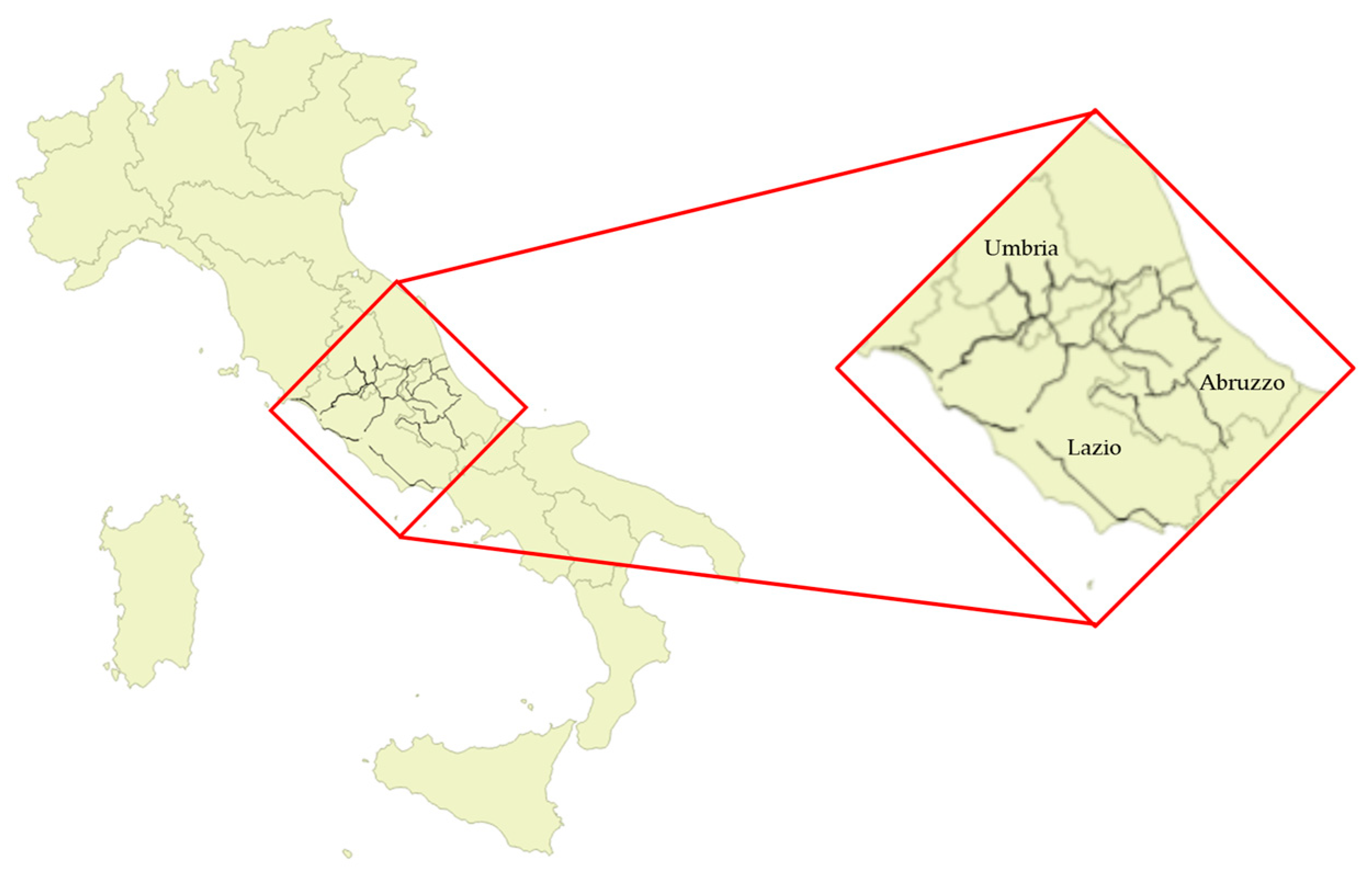
This study analyzed fifteen state roads across the regions of Lazio, Umbria, and Abruzzo, covering a total of 2000 km. These roads exhibit diverse geometric and contextual characteristics, providing a representative dataset for analysis.

The adopted methodology aims to develop a predictive model for the 85th percentile operating speed (V₈₅) on straight road sections using floating car data (FCD). The approach consists of three primary stages: (1) defining the study area and collecting relevant data, (2) processing and extracting meaningful features, and (3) developing a statistical model to estimate V₈₅ under various traffic conditions. This structured methodology ensures the accuracy, reliability, and applicability of the findings in real-world road network analysis.

3.1. Study Area and Data Collection

The study was conducted on a 2000 km road network across Italy, comprising a diverse range of state roads (Strade Statali—SS) with varying geometric characteristics. Figure 1 presents the study region where thick black lines represent the survey roads.

Table 1. Main geometric characteristics of the analyzed road segments, including total segment length, minimum and maximum curve radii, minimum and maximum tangent lengths, lane and shoulder widths, carriageway type, and the number of segments with longitudinal slopes exceeding 3%.

Road	Segment Length (km)	Min Radius (m)	Max Radius (m)	Min Tangent Length (m)	Max Tangent Length (m)	Shoulder Width (m)	Lane Width (m)	Carriageway Type	Longitudinal Slope > 3%
SS1	124	41	1836	130	7000	1–1.5	3.5–4	Mixed	in 10 sections
SS1bis	30	29	2148	121	2568	not always present	3.5–4	Single	in 5 sections
SS3	80	34	2013	139	2020	not always present	3–4	Mixed	in 14 sections
SS4	133	28	2039	120	2069	1	3–3.5	Mixed	in 11 sections
SS5	145	20	1959	120	2888	not always present	3–4	Single	in 11 sections
SS7	143	26	1971	126	35,634	0.5–1	3.5–4	Mixed	in 5 sections
SS17	151	26	2050	122	4922	0.7–1.5	3–4	Single	in 7 sections
SS79	29	75	2004	161	3751	not always present	3–4	Mixed	None
SS80	90	20	1995	137	3972	not always present	3.2–3.6	Single	in 5 sections
SS81	129	16	2023	125	1768	not always present	3.2–3.6	Single	in 12 sections
SS260	28	23	1822	133	1053	not always present	3.2–3.5	Single	in 3 sections
SS448	25.44	30	1691	144	954	not always present	≈3.5	Single	in 5 sections
SS685	70	38	2046	134	3849	≈1	3–3.5	Single	in 4 sections
SS690	39	343	2104	125	2518	≈1	≈3.5	Single	None
SS696	49	20	2162	123	1251	≈1	≈3.5	Single	in 3 sections

provides a summary of the key geometric characteristics of the rural road network segments analyzed in this study. The roads are located across three Italian regions (Lazio, Umbria, and Abruzzo) and include a wide range of configurations in terms of curvature, tangent lengths, lane and shoulder widths, and slope conditions.

The first step in the study involved interpreting the geometry of the analyzed roads and identifying straight road sections [44]. The road network was represented in the QGIS software, where each segment was attributed with a road code, secondary road name, municipality and municipality code, managing authority, segment length, center-line coordinates, and elevation. To obtain a homogeneous sample, roads were first grouped by functional class. Within each class, we retained only tangents fully bounded by two horizontal curves, discarding those that intersected junctions or direct access points. Each retained tangent was then clustered by common geometric and contextual attributes—curve radii (R₁, R₂), tangent length (L), posted speed limit, lane width, and shoulder width—derived from QGIS layers and web-mapping measurements. Both tangents ≤ 150 m and > 150 m were included, because 150 m is the threshold specified in Italian design guidelines above which drivers clearly recognize a straight alignment and stabilize their speed, reducing the influence of adjacent curves. Finally, web-based mapping tools were used to measure key cross-sectional elements (lane and shoulder widths) and to verify roadway composition. Unlike motorways, the selected state and regional roads carry mixed urban and extra-urban traffic with frequent direct accesses, factors that substantially affect vehicle speeds and driving behavior.

Data were collected using floating car data (FCD), which consists of GPS-based speed measurements from vehicles equipped with telematics devices. These datasets offer a high-resolution representation of real-world traffic behavior and provide a continuous speed profile along the study area. To enhance the reliability of the dataset, comparisons were made with fixed-location speed sensors positioned along some of the state roads. These roadside sensors record spot speeds at different locations and allow validation of the FCD-derived speed profiles [37].

3.2. Data Processing and Feature Extraction

Once the raw, GPS-based speed data were collected, a preprocessing phase was conducted to clean and structure the dataset for further analysis. The data processing workflow involved several key steps:

• Map-Matching Algorithm: A route-matching process was performed to ensure that GPS speed data accurately corresponded to specific road segments. This step mitigates potential errors in speed estimation caused by GPS drift or incorrect mapping to adjacent roads.
• Speed Profile Construction: A continuous speed diagram was generated for each road axis, providing speed values at multiple points along the segment. These profiles allowed the extraction of minimum, average, maximum, and 85th percentile speeds (V85) for each road section.
• Exploratory Data Analysis: A statistical investigation was conducted to identify the most influential factors affecting operational speeds. Key geometric features were extracted, including curvature change rate (CCR), lane width, presence of shoulders, vertical alignment, and preceding curve characteristics.
• Data Clustering: Given the heterogeneity of the study area, a clustering approach was applied to group road segments with similar geometric and contextual characteristics. This process facilitated a more refined analysis of speed variations across different conditions.

3.3. Speed Prediction Model Development

To develop a predictive model for operating speed (V₈₅) on rural, two-lane road tangents, a multistep calibration process was undertaken. The analysis considered multiple regression frameworks under three conditions, to ensure consistency with standard operational speed definitions:

• All traffic conditions;
• Free-flow conditions;
• Free-flow conditions on dry pavement.

The objective was to explore both geometric and contextual factors that influence driver behavior, with the aim of defining a generalizable model applicable across various roadway conditions. The identification of a suitable model form began with the selection and examination of relevant primary and secondary variables. Preliminary formulations were tested to assess their explanatory potential. A clustering approach was employed to segment the data, enabling more targeted regression analyses. An exploratory analysis was conducted to identify the most relevant geometric and contextual variables influencing the 85th percentile operating speed (V₈₅). The initial set of candidate variables included the radius of the preceding curve (R1), the radius of the succeeding curve (R2), tangent length (L), curvature change rate (CCR), vertical alignment (slope conditions), lane width, shoulder width, posted speed limit (V_lim), and roadway environment (e.g., urban or extra-urban setting). These variables were extracted from the road geometry database and verified through GIS tools and manual measurements using web-based mapping platforms. Each variable was assessed using univariate regressions, correlation analysis, and multivariate models to determine its statistical significance and predictive contribution. Variables with weak or inconsistent correlations across clusters were excluded from the final model to maintain generalizability and avoid overfitting.

Specifically, a divisive (top-down) clustering technique was used: the dataset, initially considered in its entirety, was iteratively divided into progressively smaller clusters, isolating homogeneous groups that aligned more closely with the regression patterns. The clustering process was conducted under the principle of exclusivity—each data element was assigned to one and only one cluster.

Five calibration approaches were tested:

• Preceding Road Segment Geometry: Initial models used the radius of the preceding horizontal curve (R1) and the tangent length (L) as predictors. Alternative regressions used the curvature change rate (CCR), a measure of roadway tortuosity. However, in all cases, predictive power remained limited.
• Both Preceding and Succeeding Geometries: The influence of both R1 and the radius of the succeeding curve (R2) was analyzed using a Koppel diagram, which identifies coherence in geometric transitions. Subgroup analyses were conducted based on the R1/R2 ratio, dividing data into four clusters depending on geometric continuity or discontinuity.
• Road Context Classification: The context of the road was introduced through the posted speed limit (V_lim) and roadway environment. Regression analyses were conducted within these subgroups to assess the role of speed regulation and road class in influencing V₈₅.
• Speed on the Preceding Element (V_{85_pe}): The 85th percentile speed on the preceding curve was used as a behavioral predictor of V₈₅ on the following tangent. This approach focused on driver adaptation rather than solely geometric parameters.
• Influence of Altimetry and Shoulder Presence: Additional regressions considered slope gradients and the presence of shoulders to evaluate their potential effects on perceived safety and speed behavior. The influence of these variables varied depending on road segment characteristics.

Figure 2 illustrates the road configuration considered in the modeling framework. It includes the radius of curvature of the preceding segment (R1), the tangent length (L), the radius of the succeeding curve (R2), and the 85th percentile speed on the preceding curve (V_{85_pe}), and the main variables used to define the predictive 85th percentile speed on the tangent segment (V₈₅).

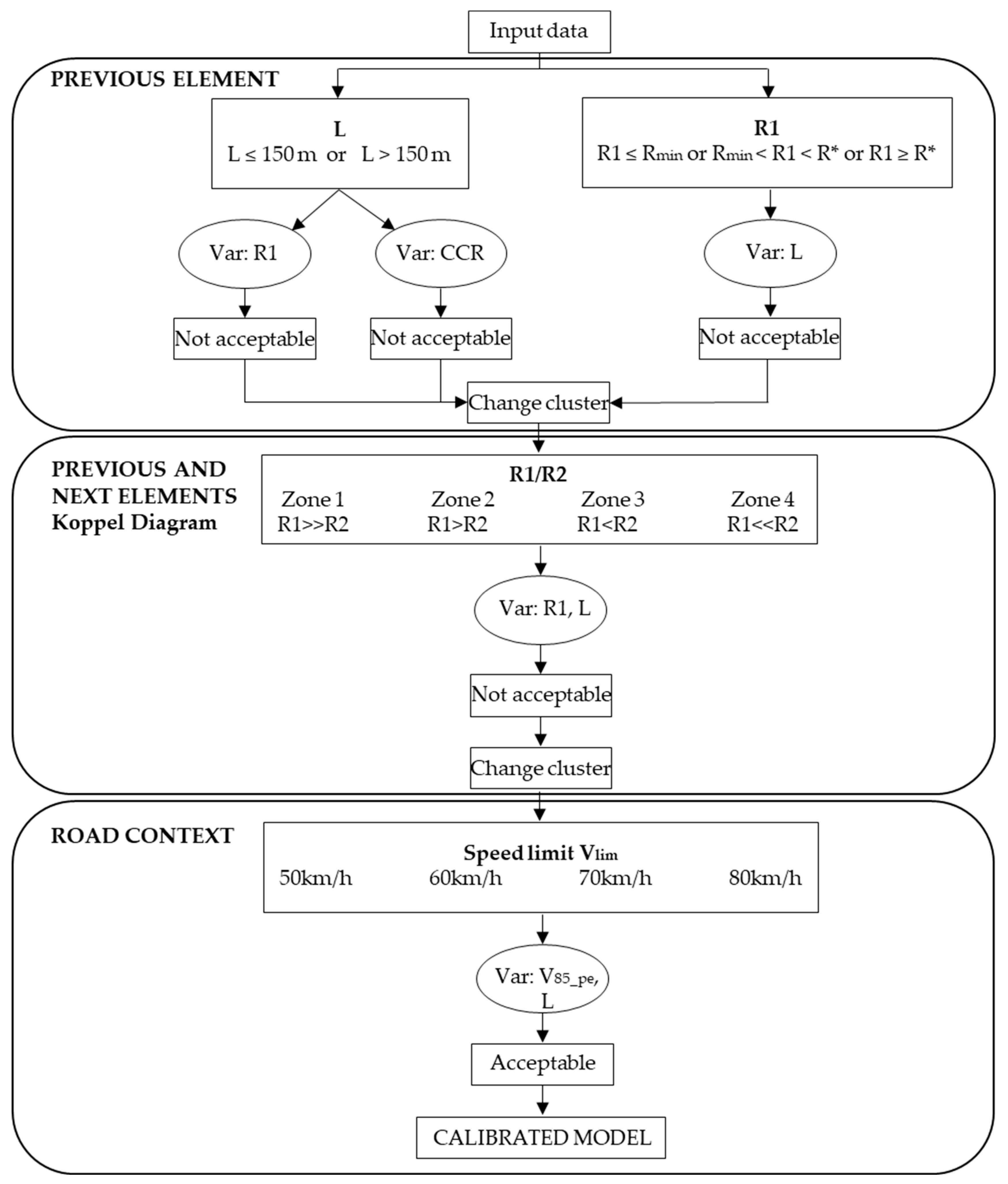
Three main procedures were developed to estimate V₈₅ on tangents (Figure 3):

• Procedure A: Estimation based on the geometry of the preceding element only (e.g., R1, L);
• Procedure B: Combined analysis of the preceding and succeeding elements, incorporating both R1 and R2;
• Procedure C: Context-aware modeling using the preceding speed (V_{85_cp}), road environment (V_lim), and geometric features (L).

Since the initial procedures did not yield satisfactory results, each subsequent model was developed as a refinement of the previous one, rather than being selected through a binary decision process. The methodological steps therefore follow a sequential logic, with each stage informed by the limitations identified in the preceding analysis.

The threshold values used for segment classification are based on design standards established in the Italian road design standards [45]. Specifically, the 150 m threshold used to differentiate straight segment lengths is based on the minimum distance required for a straight alignment to be perceived as a tangent by drivers. Accordingly, this is the minimum length applicable for rural roads with a design speed of up to 100 km/h. Moreover, the minimum radius (R_min) of 118 m corresponds to the design value for roads with the lowest permissible design speed (V_p = 60 km/h) and a maximum transverse slope of 7%. Conversely, the threshold of 437 m represents the radius for the highest design speed (V_p = 100 km/h) under the same maximum slope condition (R*). Radii between these two values reflect intermediate design speeds.

These considerations support the development of a methodological framework that integrates geometric, contextual, and behavioral variables to estimate operating speed on rural road tangents. The structure and rationale of the proposed modeling approach are outlined below, while the effectiveness and implications of the models are discussed in detail in the following section.

4. Results and Discussion

This study evaluated five calibration approaches to model the 85th percentile operating speed (V₈₅) on a total of 828 tangent segments from rural, two-lane roads. Each approach tested different combinations of geometric and contextual variables, leading to the development of several regression models.

4.1. Preceding Road Segment Geometry

Initial models, commonly used in the literature and based on geometric variables such as the radius of the preceding curve (R1) and tangent length (L), proved to be entirely unsuitable for predicting operating speed. The step-by-step selection logic has already been summarized in Figure 3, while the correlation and simple-regression results for each candidate variable are presented in

Table 2. Regression results of clusters using variable R1, differentiated by segment length (L ≤ 150 m and L > 150 m) and data type (All data, FFS, FFS dry).

	L ≤ 150 m		L > 150 m
	Speed Prediction Model	R2	Speed Prediction Model	R2
All data	V85 = 79.614 + 0.0093R1	0.056	V85 = 85.082 + 0.0066R1	0.0322
FFS	V85 = 79.6317 + 0.00944R1	0.0574	V85 = 85.126 + 0.0066R1	0.033
FFS dry	V85 = 79.695 + 0.01R1	0.0565	V85 = 85.116 + 0.0069R1	0.0314

,

Table 3. Regression results of clusters using the curvature change rate (CCR) variable, differentiated by segment length (L ≤ 150 m and L > 150 m) and data type (All data, FFS, FFS dry).

	L ≤ 150 m		L > 150 m
	Speed Prediction Model	R2	Speed Prediction Model	R2
All data	V85 = 84.59 − 0.0072CCR	0.0094	V85 = 88.153 + 0.00057CCR	0.0007
FFS	V85 = 84.638 − 0.0071CCR	0.0092	V85 = 88.178 + 0.00086CCR	0.0008
FFS dry	V85 = 84.763 − 0.0073CCR	0.0092	V85 = 88.26 + 0.0008CCR	0.001

,

Table 4. Regression results of clusters using tangent length (L) as the predictor, grouped by the radius of the preceding curve (R) and data type (All data, FFS, FFS dry).

	R ≤ 118 m		118 m < R ≤ 437 m		R > 437 m
	Speed Prediction Model	R2	Speed Prediction Model	R2	Speed Prediction Model	R2
All data	V85 = 65.259 + 0.019L	0.22	V85 = 85.751 + 0.00049L	0.0035	V85 = 87.161 + 0.005L	0.1385
FFS	V85 = 65.259 + 0.018L	0.22	V85 = 85.512 + 0.00139L	0.0221	V85 = 87.258 + 0.00486L	0.1379
FFS dry	V85 = 65.248 + 0.019L	0.232	V85 = 85.61 + 0.0014L	0.0218	V85 = 87.384 + 0.005L	0.1369

,

Table 5. Regression results for different zones using both the radius of the preceding curve (R1) and tangent length (L) as predictors, grouped by data type (All data, FFS, FFS dry).

	Zone 1		Zone 2
	Speed Prediction Model	R2	Speed Prediction Model	R2
All data	V85 = 75.258 + 0.006R1 + 0.0010L	0.07	V85 = 85.466 + 0.005R1 + 0.0029L	0.059
FFS	V85 = 75.198 + 0.006R1 + 0.0010L	0.072	V85 = 85.496 + 0.005R1 + 0.0029L	0.059
FFS dry	V85 = 75.691 + 0.006R1 + 0.0009L	0.067	V85 = 85.359 + 0.005R1 + 0.0029L	0.061
	Zone 3		Zone 4
	Speed Prediction Model	R2	Speed Prediction Model	R2
All data	V85 = 82.422 + 0.013R1 + 0.0022L	0.073	V85 = 61.571 + 0.095R1 + 0.0034L	0.495
FFS	V85 = 82.484 + 0.013R1 + 0.0022L	0.074	V85 = 61.602 + 0.095R1 + 0.0034L	0.494
FFS dry	V85 = 82.627 + 0.013R1 + 0.0021L	0.071	V85 = 61.906 + 0.094R1 + 0.0034L	0.496

,

Table 6. Regression results for different posted speed limits (V_lim), using V_{85_pe} (calculated curve speed) and tangent length (L) as predictors. Results are grouped by data type (All data, free-flow speed (FFS), and FFS under dry conditions) and include model coefficients, coefficient of determination (R²), root mean square error (RMSE), and mean absolute error (MAE).

Vlim = 50 km/h
	Speed Prediction Model	R2	RMSE (km/h)	MAE (km/h)
All data	V85 = 13.433 + 0.859V85cp + 0.0017L	0.829	6.8	5.2
FFS	V85 = 13.65 + 0.856V85cp + 0.0017L	0.829	6.7	5.1
FFS dry	V85 = 14.836 + 0.843V85cp + 0.0016L	0.834	6.6	4.9
Vlim = 60 km/h
	Speed Prediction Model	R2	RMSE (km/h)	MAE (km/h)
All data	V85 = 23.311 + 0.739V85cp − 0.0008L	0.691	7.5	5.9
FFS	V85 = 22.501 + 0.749V85cp − 0.0007L	0.695	7.3	5.7
FFS dry	V85 = 22.975 + 0.74V85cp − 0.0006L	0.688	7.6	5.8
Vlim = 70 km/h
	Speed Prediction Model	R2	RMSE (km/h)	MAE (km/h)
All data	V85 = 15.287 + 0.845V85cp + 0.0044L	0.846	6.2	4.7
FFS	V85 = 15.378 + 0.844V85cp + 0.0045L	0.847	6.1	4.6
FFS dry	V85 = 15.801 + 0.836V85cp + 0.0047L	0.837	6.4	4.8
Vlim = 90 km/h
	Speed Prediction Model	R2	RMSE (km/h)	MAE (km/h)
All data	V85 = 17.843 + 0.81V85cp + 0.0062L	0.944	5.1	3.9
FFS	V85 = 17.64 + 0.812V85cp + 0.0062L	0.945	5.0	3.8
FFS dry	V85 = 24.497 + 0.732V85cp + 0.0053L	0.927	5.3	4.1

,

Table 7. Regression results based on gradient (i), grouped by tangent length (L ≤ 150 m and L > 150 m), using R1 as the predictor. A threshold value of 3% was used to distinguish between low and high slope segments.

	L ≤ 150 m		L > 150 m
	Speed Prediction Model	R2	Speed Prediction Model	R2
FFS dry	V85 = 79.695 + 0.01R1	0.056	V85 = 85.116 + 0.0069R1	0.031
i < 3%	V85 = 80.587 + 0.005R1	0.023	V85 = 84.201 + 0.008R1	0.046
i ≥ 3%	V85 = 76.385 + 0.023R1	0.175	V85 = 86.848 + 0.009R1	0.048

and

Table 8. Regression results based on the presence of shoulders, using R1 as the predictor and grouped by tangent length (L ≤ 150 m and L > 150 m).

	L ≤ 150 m		L > 150 m
	Speed Prediction Model	R2	Speed Prediction Model	R2
Shoulders	V85 = 82.929 + 0.011R1	0.095	V85 = 87.745 + 0.005R1	0.023
No Shoulders	V85 = 84.924 − 0.001R1	0.0017	V85 = 82.711 + 0.009R1	0.0572

below. As shown in Table 2, the coefficients of determination (R²) for these regressions remain consistently below 0.06, regardless of the segment length or data type. These results confirm the very limited explanatory power of such models, highlighting their inadequacy when relying solely on geometric parameters.

Additional geometric variables, such as the curvature change rate (CCR), were also introduced in an attempt to improve model performance. However, as shown in Table 3, the models yielded extremely low coefficients of determination (R² < 0.01), further confirming the weak correlation between CCR and operating speed. These findings reinforce the inadequacy of traditional geometric indicators—whether R1, L, or CCR—as reliable predictors of speed behavior.

Tangents were analyzed by clustering segments according to the radius of the preceding curve, using tangent length (L) as the only independent variable in the regression models. As shown in Table 4, while slightly higher coefficients of determination were observed in clusters with very sharp curves (R ≤ 118 m, R² ≈ 0.22), the overall explanatory power remained low or negligible for larger radius ranges (R² < 0.14 for R > 437 m).

These results confirm that defining clusters solely by radius and relying exclusively on tangent length is insufficient for accurately predicting operating speed.

4.2. Combined Preceding and Succeeding Geometry

To capture the full transition of driver behavior through a tangent section, both the preceding curve radius (R1) and the succeeding one (R2) were introduced. Subgroup analyses based on the R1/R2 ratio were conducted, dividing data into clusters depending on geometric continuity or discontinuity. Different user behaviors (in terms of average V₈₅ along the tangent) are expected depending on the group considered:

• Zone 1 R1 >> R2: If the driver comes from a curve with a very large radius and faces a curve with a much smaller radius, they are likely to avoid accelerating significantly along the tangent.
• Zone 2 R1 > R2: If the driver comes from a curve with a larger radius than the following one, but of similar magnitude, they may accelerate moderately along the tangent.
• Zone 3 R1 < R2: If the driver comes from a curve with a smaller radius than the following one, again of similar magnitude, they may accelerate slightly more than in case 2.
• Zone 4 R1 << R2: If the driver comes from a curve with a very small radius and then faces a curve with a much larger radius, they are likely to accelerate substantially along the tangent, perceiving the geometry as less constraining.

To improve model accuracy, combined regressions using both the radius of the preceding curve (R1) and tangent length (L) were tested across different zones (Table 5).

The results shown in Table 5 reveal that in Zones 1 to 3, where operating speeds are generally higher, the combined use of R1 and L provides only marginal improvements in explanatory power, with R² values below 0.08. However, in Zone 4—characterized by significantly lower operating speeds due to transitions from sharp curves (small R1) to much flatter downstream geometry (large R2)—the model demonstrates a substantially stronger predictive performance, with R² values consistently around 0.495 across all traffic conditions. This notable improvement indicates that in lower-speed contexts, drivers are more sensitive to the combined geometric configuration, particularly when faced with a sharp deceleration followed by a long tangent and a gentler succeeding curve. The interaction between the radius of the preceding curve (R1) and tangent length (L) becomes more influential in shaping speed behavior, likely due to increased cognitive load and speed adaptation needs in these transitional segments. This confirms that geometric continuity and driver anticipation play a critical role in speed selection under constrained conditions, justifying the stronger correlation observed in this specific geometric zone.

4.3. Road Context Classification

Incorporating contextual elements such as the posted speed limit (V_lim) and roadway classification aimed to account for environmental influences beyond pure geometry. Regression analyses within these subgroups yielded notable, though variable, improvements in explanatory power. For instance, in the 50 km/h speed limit group, the use of log-transformed tangent length (log L) as an independent variable produced R² values exceeding 0.45, indicating a moderate to strong correlation between geometric context and driver speed behavior in lower-speed environments. This suggests that in urban or peri-urban contexts—often associated with this speed limit—drivers are more responsive to road geometry when speed expectations are lower and surrounding constraints (e.g., access points, limited visibility) amplify the influence of tangent length on speed choice. These findings support the relevance of incorporating contextual classifications in speed prediction models, especially for infrastructure types with higher behavioral variability.

4.4. Speed on the Preceding Element (V_{85_pe})

A significant improvement in model performance was achieved by introducing the 85th percentile speed on the preceding curve (V_{85_pe}) as a predictor, reflecting the driver’s response to the road segment just traveled. Consequently, the regression model was revised to replace the geometric parameters of the preceding curve with its observed operating speed, capturing behavioral rather than purely geometric influences (Table 6).

This model demonstrated coefficients of determination (R²) consistently higher than 0.68 across all speed limit categories, with values exceeding 0.829 for speed limits of 50, 70, and 90 km/h, and reaching as high as 0.927 for the highest speed class. These results indicate a strong predictive relationship between the preceding element speed (V_{85_pe}), tangent length (L), and the actual observed operating speed (V₈₅). The high R² values suggest that the combined use of these two variables effectively captures the variability in driving behavior across different roadway environments and speed regimes, making this model a reliable tool for estimating operating speeds in design and safety evaluations.

In addition to R², model performance was also evaluated using the root mean square error (RMSE) and mean absolute error (MAE). These indicators provide a more robust assessment of prediction accuracy and allow for a clearer comparison among the proposed approaches. Lower values indicate better fit.

4.5. Influence of Vertical Alignment and Shoulder Presence

Additional stratified models were developed to test the impact of longitudinal slope (i.e., gradients above or below 3%) and the presence or absence of road shoulders. It can be observed in Table 7 that longitudinal slopes greater than 3% impact speed but not significantly, likely because the analyzed vehicles are mostly passenger cars with high specific power.

Similarly, road shoulders seem to affect drivers’ perception of safety, but the results indicate that their effect is not consistent, as can be seen in Table 8.

When the tangent is long, the driver is influenced by the presence of a shoulder and can choose their speed more freely. In contrast, without a shoulder, the driver’s behavior is more constrained, and the correlation increases.

Although these factors influenced driver behavior in specific scenarios, their contribution to a generalizable model was limited due to data quality and variability. The analysis indicates that geometric parameters alone are insufficient to accurately predict operating speeds on rural tangents. Instead, models that incorporate behavioral indicators, such as the speed on the preceding curve, and contextual variables offer a more comprehensive and reliable estimation framework. This methodological framework enables a data-driven assessment of speed consistency on road networks, supporting infrastructure design and road safety analysis.

4.6. Speed Prediction Model Validation

To assess the reliability and generalizability of the developed model, a validation phase was carried out using data from additional samples of road segments not included in the calibration phase. The selected roadways were chosen based on the availability of speed limit information and recorded vehicle speeds under free-flow, dry conditions.

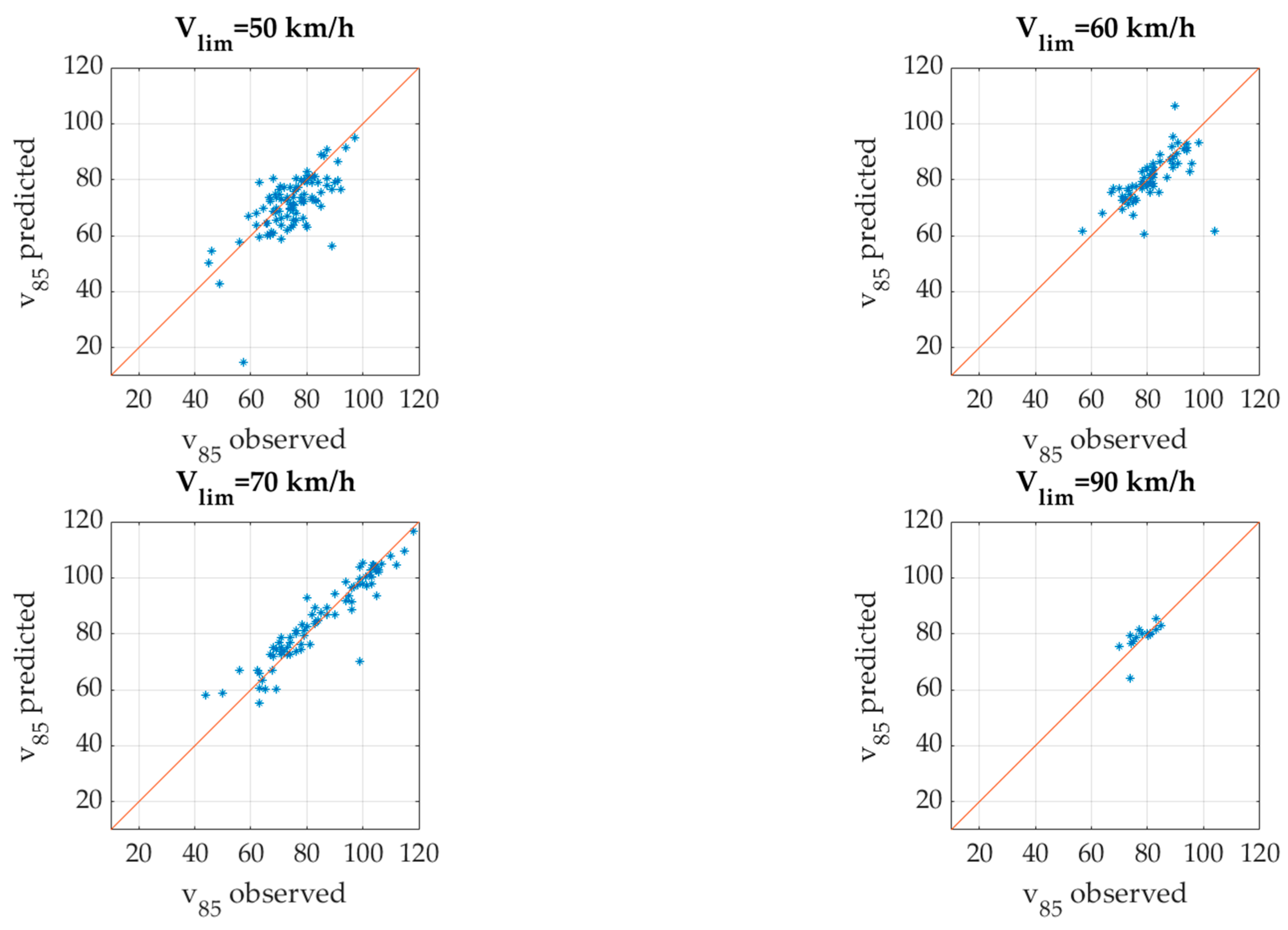
The validation process involved applying the final set of regression equations in FFS on dry pavement, particularly those incorporating the 85th percentile speed on the preceding element (V_{85_pe}) and the tangent length (L), to predict operating speeds on these new road segments. The predicted V₈₅ values were then compared with observed data collected from floating car data (FCD) recordings. The results can be observed in Figure 4.

The comparison results showed a strong alignment between calculated and observed values, as evidenced by the distribution of points near the bisector line in the prediction-validation plots. Importantly, the data points were spread both above and below the bisector, indicating that the model does not exhibit a systematic tendency to overestimate or underestimate operating speeds.

The analysis of the proposed models showed that geometric parameters alone are insufficient to fully explain variations in operating speed. Drivers tend to adapt their speed based on prior experience and perceived risk, leading to behaviors that are not fully captured by traditional geometric indicators. While variables such as curvature, lane width, and vertical alignment showed limited and context-dependent influence on V₈₅, the most significant predictors were the 85th percentile speed on the preceding curve and the length of the tangent segment. As shown in Table 6, these variables yielded coefficients of determination (R²) ranging from 0.688 to 0.945 across different posted speed limits and traffic conditions, indicating strong and consistent predictive power. Additionally, the inclusion of posted speed limits substantially improved model performance, demonstrating the importance of contextual factors. These findings support the robustness of the proposed model and its applicability to different road contexts. They also confirm the effectiveness of using behavioral indicators—such as V₈₅ on the preceding element—over purely geometric parameters in predicting speed behavior along rural tangents. From a logical and operational standpoint, the final model structure reflects the influence of road geometry on driver behavior in transition zones, particularly the interaction between curves and subsequent tangents. The inclusion of variables such as the preceding curve radius (R1) and tangent length (L) is consistent with the literature findings and with the observed gradual speed adaptation patterns in the FCD data. The exclusion of certain contextual variables (e.g., lane width, shoulder width) from the final model is justified by their limited statistical contribution and by the need to ensure model robustness and generalizability.

The proposed speed prediction models offer concrete opportunities for implementation in both research and operational contexts. From a traffic engineering perspective, they can be used to support safety audits and design consistency evaluations by identifying segments where actual driving behavior significantly deviates from expected values. Road authorities and planners can also apply the model during the geometric design or rehabilitation phases to assess whether design assumptions align with behavior-based speed predictions derived from real-world data. Additionally, the models can be integrated into traffic simulation platforms and digital twins to generate more realistic speed profiles along rural roads. In the context of emerging mobility technologies, such as connected and autonomous vehicles (CAVs), the model can be embedded in decision-making algorithms to improve speed control, risk prediction, and motion planning on roadways with limited digital infrastructure.

Overall, the methodology is scalable and adaptable to different regional datasets, enabling broad applicability for infrastructure planning, policy evaluation, and intelligent transportation systems.

5. Conclusions

This study presents a comprehensive methodology for modeling operating speed (V₈₅) on straight sections of rural roads by integrating geometric features, contextual variables, and behavioral indicators derived from floating car data (FCD). The analysis demonstrates that relying solely on geometric parameters—such as the radius of the preceding curve, tangent length, and curvature change rate—is insufficient for accurately predicting driver behavior along straight segments.

Among the five calibration approaches tested, the most significant improvement in model performance was achieved by incorporating the 85th percentile speed on the preceding element (V_{85_pe}) as a behavioral predictor. This variable effectively captured the driver’s adaptation to road geometry and conditions, reflecting the influence of the previously traveled segment. The resulting regression models consistently yielded high correlation coefficients (R² between 0.73 and 0.93), outperforming those based exclusively on geometric descriptors.

The validation phase, conducted on independent road segments, confirmed the robustness and generalizability of the proposed models. Predicted V₈₅ values aligned closely with observed speeds, without systematic over- or underestimation. These outcomes reinforce the model’s applicability to diverse road environments and support its integration into traffic safety assessments and infrastructure design practices.

The methodological framework developed in this research enables a data-driven evaluation of speed consistency, facilitating the identification of critical segments and the design of targeted safety interventions. By leveraging FCD and statistical modeling, the study offers valuable insights into real-world driving behavior, supporting the development of resilient and adaptive traffic systems.

Furthermore, the developed models—capable of estimating realistic operating speeds by integrating both geometric and behavioral conditions—offer valuable opportunities for practical implementation, particularly within the realm of connected and autonomous vehicles (CAVs). Predictive knowledge of expected traffic flow speeds can support autonomous systems in optimizing trajectory planning, ensuring smooth and safe maneuvers while adapting to the anticipated behaviors of surrounding vehicles. Such integration is especially relevant in scenarios with limited infrastructure connectivity or reduced visibility, where algorithms for adaptive cruise control (ACC) and predictive speed adaptation (PSA) must rely on robust, context-aware speed prediction models.

The methodological framework presented in this study provides a strong foundation for further research aimed at enhancing model accuracy, applicability, and generalizability. Future developments will focus on incorporating a broader set of behavioral variables—such as driver demographics, risk perception, and experience—alongside critical environmental conditions (e.g., weather, lighting, and visibility). Additionally, the inclusion of network-related characteristics, such as traffic flow variability and pavement conditions, will support more comprehensive and adaptive modeling approaches.

Finally, extending the validation process to encompass a wider variety of road types and geographic contexts will be essential to ensure the robustness of the proposed models. These future directions are key to refining their operational relevance and enabling their integration into advanced vehicle control systems and intelligent transport infrastructure in mixed-traffic environments.

References

- Abdelkader, G.; Elgazzar, K.; Khamis, A. Connected Vehicles: Technology Review, State of the Art, Challenges and Opportunities. Sensors 2021, 21, 7712. [Google Scholar] [CrossRef] [PubMed]
- Liu, C.; Zyryanov, V.; Topilin, I.; Feofilova, A.; Shao, M. Investigating the Impacts of Autonomous Vehicles on the Efficiency of Road Network and Traffic Demand: A Case Study of Qingdao, China. Sensors 2024, 24, 5110. [Google Scholar] [CrossRef] [PubMed]
- Jiang, W.; Luo, J. Big Data for Traffic Estimation and Prediction: A Survey of Data and Tools. Appl. Syst. Innov. 2022, 5, 23. [Google Scholar] [CrossRef]
- Lamm, R.; Psarianos, B.; Mailaender, T.; Choueiri, E.M.; Heger, R.; Steyer, R. Highway Design and Traffic Safety Engineering Handbook, 1st ed.; McGraw-Hill: New York, NY, USA, 1999; ISBN 0070382956. [Google Scholar]
- Abbas, S.K.S.; Adnan, M.A.; Endut, I.R. Exploration of 85th percentile operating speed model on horizontal curve: A case study for two-lane rural highways. Procedia Soc. Behav. Sci. 2011, 16, 352–363. [Google Scholar] [CrossRef]
- Godumala, D.T.; Ravi Shankar, K.V.R. Geometric Design Consistency Model for Evaluating Safety at Horizontal Curves on Two-Lane Rural Highways Under Mixed Traffic Conditions. J. Inst. Eng. India Ser. A 2024, 105, 307–316. [Google Scholar] [CrossRef]
- Saedi, H.; Abdi Kordani ADivandari, H. Improving safety in rural highways horizontal curves using geometric design consistency evaluation criteria based on operating speed modeling. Innov. Infrastruct. Solut. 2024, 9, 134. [Google Scholar] [CrossRef]
- ISTAT. Incidenti Stradali in Italia; Istituto Nazionale di Statistica: Rome, Italy, 2023. [Google Scholar]
- Altintasi, O.; Tuydes-Yaman, H.; Tuncay, K. Quality of Floating Car Data (FCD) as a surrogate measure for urban arterial speed. Can. J. Civ. Eng. 2019, 46, 1187–1198. [Google Scholar] [CrossRef]
- De Fabritiis, C.; Ragona, R.; Valenti, G. Traffic estimation and prediction based on real-time floating car data. In Proceedings of the 11th International IEEE Conference on Intelligent Transportation Systems, Beijing, China, 12–15 October 2008; pp. 197–203. [Google Scholar] [CrossRef]
- Houbraken, M.; Logghe, S.; Audenaert, P.; Colle, D.; Pickavet, M. Examining the Potential of Floating Car Data for Dynamic Traffic Management. IET Intell. Transp. Syst. 2018, 12, 335–344. [Google Scholar] [CrossRef]
- Jurewicz, C.; Espada, I.; Makwasha, T.; Han, C.; Alawi, H.; Ambros, J. Validation and applicability of floating car speed data for road safety. In Proceedings of the 2017 Australasian Road Safety Conference, Perth, Australia, 10–12 October 2017. [Google Scholar]
- Guo, Z.; Zhou, X.; Yan, Y.; Zhang, Q.; Chen, Y. Operating speed prediction model based on highway alignment spacial geometric properties. In Proceedings of the ICCTP 2010: Integrated Transportation Systems: Green, Intelligent, Reliable, Beijing, China, 4–8 August 2010; pp. 961–970. [Google Scholar] [CrossRef]
- Boroujerdian, A.M.; Seyedabrishami, E.; Akbarpour, H. Analysis of geometric design impacts on vehicle operating speed on two-lane rural roads. Procedia Eng. 2016, 161, 1144–1151. [Google Scholar] [CrossRef]
- Gibreel, G.M.; Easa, S.M.; El-Dimeery, I.A. Prediction of operating speed on three-dimensional highway alignments. J. Transp. Eng. 2001, 127, 21–30. [Google Scholar] [CrossRef]
- Capacità Delle Reti Infrastrutturali Di Trasporto. Available online: https://indicatoriambientali.isprambiente.it/it/trasporti/capacita-delle-reti-infrastrutturali-di-trasporto (accessed on 17 March 2025).
- Incidenti Stradali Anno 2022. Available online: https://www.istat.it/it/files/2023/07/REPORT_INCIDENTI_STRADALI_2022_IT.pdf (accessed on 17 March 2025).
- Rana, M.M.; Hossain, K. Connected and Autonomous Vehicles and Infrastructures: A Literature Review. Int. J. Pavement Res. Technol. 2023, 16, 264–284. [Google Scholar] [CrossRef]
- Sadid, H.; Antoniou, C. Modelling and simulation of (connected) autonomous vehicles longitudinal driving behavior: A state-of-the-art. IET Intell. Transp. Syst. 2023, 17, 1051–1071. [Google Scholar] [CrossRef]
- Ahmed, H.U.; Huang, Y.; Lu, P.; Bridgelall, R. Technology developments and impacts of connected and autonomous vehicles: An overview. Smart Cities 2022, 5, 382–404. [Google Scholar] [CrossRef]
- Gong, H.; Stamatiadis, N. Operating speed prediction models for horizontal curves on rural four-lane highways. Transp. Res. Rec. 2008, 2075, 1–7. [Google Scholar] [CrossRef]
- Morris, C.M.; Donnell, E.T. Passenger car and truck operating speed models on multilane highways with combinations of horizontal curves and steep grades. J. Transp. Eng. 2014, 140, 04014058. [Google Scholar] [CrossRef]
- Camacho-Torregrosa, F.J.; Pérez-Zuriaga, A.M.; Campoy-Ungría, J.M.; García-García, A. New geometric design consistency model based on operating speed profiles for road safety evaluation. Accid. Anal. 2013, 61, 33–42. [Google Scholar] [CrossRef]
- Tüydeş Yaman, H.; Kocamaz, K.; Tuncay, K.; Çınar, B. On Strategies Improving Accuracy of Speed Prediction from Floating Car Data (FCD). In Proceedings of the 14th International Congress on Advances in Civil Engineering (ACE 2020-21), Istanbul, Turkey, 6–8 September 2021; Yıldız Technical University: Istanbul, Turkey, 2021; pp. 1–8. [Google Scholar]
- Mena-Oreja, J.; Gozalvez, J. On the impact of floating car data and data fusion on the prediction of the traffic density, flow and speed using an error recurrent convolutional neural network. IEEE Access 2021, 9, 133710–133724. [Google Scholar] [CrossRef]
- Hassan, Y.; Easa, S.M. Effect of vertical alignment on driver perception of horizontal curves. J. Transp. Eng. 2003, 129, 399–407. [Google Scholar] [CrossRef]
- Abbas, S.K.S.; Adnan, M.A.; Endut, I.R. An investigation of the 85th percentile operating speed models on horizontal and vertical alignments for two-lane rural highways: A case study. J. Inst. Eng. 2012, 32–40. [Google Scholar]
- Krammes, R.A.; Brackett, R.Q.; Shafer, M.A.; Ottesen, J.L.; Anderson, I.B.; Fink, K.L.; Messer, C.J. Horizontal Alignment Design Consistency for Rural Two-Lane Highways; (No. FHWA-RD-94-034); Federal Highway Administration: Washington, DC, USA, 1995. [Google Scholar]
- Cafiso, S.; Cerni, G. New approach to defining continuous speed profile models for two-lane rural roads. Transp. Res. Rec. 2012, 2309, 157–167. [Google Scholar] [CrossRef]
- Almeida, R.; Vasconcelos, L.; Silva, A.B. A speed model for curves of two-lane rural highways based on continuous speed data. In Transport Infrastructure and Systems; CRC Press: Boca Raton, FL, USA, 2017; pp. 177–184. [Google Scholar]
- D’Andrea, A.; Carbone, F.; Salviera, S.; Pellegrino, O. The most influential variables in the determination of V85 speed. Procedia-Soc. Behav. Sci. 2012, 53, 633–644. [Google Scholar] [CrossRef]
- Odhams, A.M.; Cole, D.J. Models of driver speed choice in curves. In Proceedings of the 7th International Symposium on Advanced Vehicle Control, Arnhem, The Netherlands, 23–27 August 2004; pp. 1–6. [Google Scholar]
- Dell’Acqua, G. European speed environment model for highway design-consistency. Mod. Appl. Sci. 2012, 6, 1. [Google Scholar] [CrossRef]
- Polus, A.; Fitzpatrick, K.; Fambro, D.B. Predicting operating speeds on tangent sections of two-lane rural highways. Transp. Res. Rec. 2000, 1737, 50–57. [Google Scholar] [CrossRef]
- Del Serrone, G.; Cantisani, G.; Peluso, P. Speed data collection methods: A review. Transp. Res. Procedia 2023, 69, 512–519. [Google Scholar] [CrossRef]
- Sohr, A.; Wagner, P. Short term traffic prediction using cluster analysis based on floating car data. In Proceedings of the 15th World Congress on ITS, New York, NY, USA, 16–20 November 2008; pp. 1–4. [Google Scholar]
- Cantisani, G.; Del Serrone, G.; Peluso, P. Reliability of Historical Car Data for Operating Speed Analysis along Road Networks. Sci 2022, 4, 18. [Google Scholar] [CrossRef]
- Del Serrone, G.; Cantisani, G.; Peluso, P.; Coppa, I.; Mancinetti, M.; Bianchini, B. Road Infrastructure Safety Management: Proactive Safety Tools to Evaluate Potential Conditions of Risk. Transp. Res. Procedia 2023, 69, 711–718. [Google Scholar] [CrossRef]
- Song, C.; Jia, H. Multi-State car-following behavior simulation in a mixed traffic flow for ICVs and MDVs. Sustainability 2022, 14, 13562. [Google Scholar] [CrossRef]
- Huang, K.; Di, X.; Du, Q.; Chen, X. Stabilizing Traffic via Autonomous Vehicles: A Continuum Mean Field Game Approach. In Proceedings of the 22nd IEEE International Conference on Intelligent Transportation Systems (ITSC), Auckland, New Zealand, 27–30 October 2019. [Google Scholar]
- Zheng, S.; Jiang, R.; Zhang, H.M.; Tian, J.; Yan, R.; Jia, B.; Gao, Z. Oscillation growth in mixed traffic flow of human driven vehicles and automated vehicles: Experimental study and simulation. In Proceedings of the International Conference on Traffic and Granular Flow, Singapore, 15–17 October 2022; pp. 267–274. [Google Scholar]
- Zheng, Y.; Wang, J.; Li, K. Smoothing traffic flow via control of autonomous vehicles. IEEE Internet Things J. 2020, 7, 3882–3896. [Google Scholar] [CrossRef]
- Anastassov, A.; Jang, D.; Giurgiu, G. Driving speed profiles for autonomous vehicles. In Proceedings of the 2017 IEEE Intelligent Vehicles Symposium (IV), Redondo Beach, CA, USA, 11–14 June 2017; pp. 1446–1451. [Google Scholar]
- Cantisani, G.; Del Serrone, G. Procedure for the Identification of Existing Roads Alignment from Georeferenced Points Database. Infrastructures 2021, 6, 2. [Google Scholar] [CrossRef]
- Ministero delle Infrastrutture e dei Trasporti. Decreto Ministeriale 5 Novembre 2001, n. 6792 (S.O. n.5 alla G.U. n.3. del 4.1.02). Norme Funzionali e Geometriche per la Costruzione Delle Strade. Available online: https://www.mit.gov.it/nfsmitgov/files/media/normativa/2017-09/decreto_ministeriale_protocollo_6792_del_5-11-2001.pdf (accessed on 16 June 2025).
Figure 1.
Study region: approximately 2000 km of state roads located within the Italian regions of Lazio, Umbria, and Abruzzo.
Figure 2.
Schematic representation of the geometric configuration used in the speed prediction model.
Figure 3.
Schematic representation of the three procedures used to model V85 on straight road sections.
Figure 4.
Comparison between observed and predicted V85 operating speeds for different posted speed limits (Vlim = 50, 60, 70, and 90 km/h). The diagonal red line represents perfect agreement between recorded and calculated values.