Article

Research on a Two-Stage Human-like Trajectory-Planning Method Based on a DAC-MCLA Network

by
Hao Xu
,
Guanyu Zhang
and
Huanyu Zhao
*
College of Instrument Science and Electrical Engineering, Jilin University, 938 Xi Minzhu Street, Changchun 130061, China
*
Author to whom correspondence should be addressed.
Vehicles 2025, 7(3), 63; https://doi.org/10.3390/vehicles7030063
Submission received: 17 May 2025 / Revised: 13 June 2025 / Accepted: 14 June 2025 / Published: 24 June 2025

Abstract

Due to the complexity of the unstructured environment and the high-level requirement of smoothness when a tracked transportation vehicle is traveling, making the vehicle travel as safely and smoothly as when a skilled operator is maneuvering the vehicle is a critical issue worth studying. To this end, this study proposes a trajectory-planning method for human-like maneuvering. First, several field equipment operators are invited to manipulate the model vehicle for obstacle avoidance driving in an outdoor scene with densely distributed obstacles, and the manipulation data are collected. Then, in terms of the lateral displacement, by comparing the similarity between the data as well as the curvature change degree, the data with better smoothness are screened for processing, and a dataset of human manipulation behaviors is established for the training and testing of the trajectory-planning network. Then, using the dynamic parameters as constraints, a two-stage planning approach utilizes a modified deep network model to map trajectory points at multiple future time steps through the relationship between the spatial environment and the time series. Finally, after the experimental test and analysis with multiple methods, the root-mean-square-error and the mean-average-error indexes between the planned trajectory and the actual trajectory, as well as the trajectory-fitting situation, reveal that this study’s method is capable of planning long-step trajectory points in line with human manipulation habits, and the standard deviation of the angular acceleration and the curvature of the planned trajectory show that the trajectory planned using this study’s method has a satisfactory smoothness.

1. Introduction

The field of autonomous driving has made great progress over the past few decades. However, unstructured environments lack a clear definition and delineation of space, order, and rules and have dense, complex distributions of obstacles. In unstructured environments, commonly used tracked transportation vehicles have high-level requirements for driving stability, due to their high centers of gravity, and experience increased difficulty in driving safely and smoothly. How to make a vehicle travel at a level like that when a skilled operator controls a vehicle to manipulate the vehicle to drive safely and smoothly is a problem that needs to be considered [1,2,3]. This problem can be solved in the motion-planning module, that is, by planning trajectories that match human manipulation behavior [4].
Traditional rule-based planning methods (heuristic search [5], stochastic probability [6], and geometric planning [7,8]) need to use environmental information, the vehicle’s state, and other information as constraints when they are applied to generate trajectories through the constructed physical expression model. However, when the driving conditions are more complex, this type of method encounters the problem of the conflict between the rules and forced simplification of the model, so designing rules that meet human expectations when facing complex unstructured environments is more difficult [9,10,11,12,13]. Experienced human controllers can make corresponding decisions for changing scenarios to control the vehicle safely and smoothly, so learning driving strategies from human control data and then planning trajectories that meet human control habits are worthy research methods.
With the development of artificial intelligence, learning-based methods have been widely studied, among which imitation-learning methods directly copy human drivers’ actions through holistic neural networks and massive offline-driving datasets, acquire operational skills from human demonstrations, and then replicate the learned skills in new scenarios. However, this method suffers from distributional shifts from training to deployment, which are difficult to mitigate [14,15,16].
Reinforcement-learning methods study human manipulation strategies by means of manipulators interacting with the environment, in which a predesigned reward function is optimized by constant trial and error to maximize the cumulative rewards, which can lead to the problems of a long optimization-learning time and greater difficulty in accurately modeling the environment as well as manually designing an appropriate reward function [17,18,19,20]. The inverse-reinforcement-learning method avoids manually designing the cost function and can learn the underlying cost function from the data demonstrated by the operator to address the ambiguities or uncertainties inherent in human demonstrations; however, it requires the use of a relatively simple model during training, and the training efficiency is low, which limits the application of this method to the aspect of extracting human manipulation features [21].
Other learning-based methods include the spline-based via-point model [22], the hidden Markov model [23], the Gaussian mixture model [24], and dynamic movement primitives [25]. These methods find the weights of the cost function by obtaining empirical data by means of human demonstrations and then narrowing down the deviation values of the matching features between the optimal trajectory of the reward function and the empirical data. However, a widespread problem is that the optimal trajectory chosen may be vastly different from that of the human demonstration in the same situation [4].
Deep-learning-based methods have been widely used recently due to their prominent learning capabilities. Among them, data-driven methods can learn manipulation techniques from human manipulation data and have a natural advantage in realizing human-like trajectory planning [26]. Because convolutional neural networks (CNNs) have a strong understanding of spatial scenes and the trajectory points in the data have a strong correlation in terms of time series, this study uses an improved CNN network with a multiple-time-step sliding prediction to plan the trajectory points in the future long time series so that the vehicle can be driven safely and smoothly while providing a safe decision-making time for local dynamic obstacle avoidance [27,28,29].
In this study, first, 15 manipulators are invited to manipulate a real tracked model vehicle to avoid obstacles, drive in an unstructured environment with densely distributed obstacles, and collect manipulation data during driving. Next, the data are cleaned and grouped for processing to construct a human manipulation behavior dataset. Then, the DenseNet Attention Compensation network (DAC) is used for the primary planning of future trajectory points; the element-by-element Multiplication Cell-State LSTM Attention network (MCLA) is used for secondary planning based on the correlation of the primary planning trajectory points in the time series. The vehicle’s dynamic parameters are used as constraints to enhance trajectory-planning accuracy. The main contributions of this study are as follows:
  • A number of field equipment manipulators was invited to control the vehicle and collect manipulation data. The data were screened based on the similarity of transverse displacement and the degree of curvature vatiation to construct a dataset representing human manipulation behaviors.
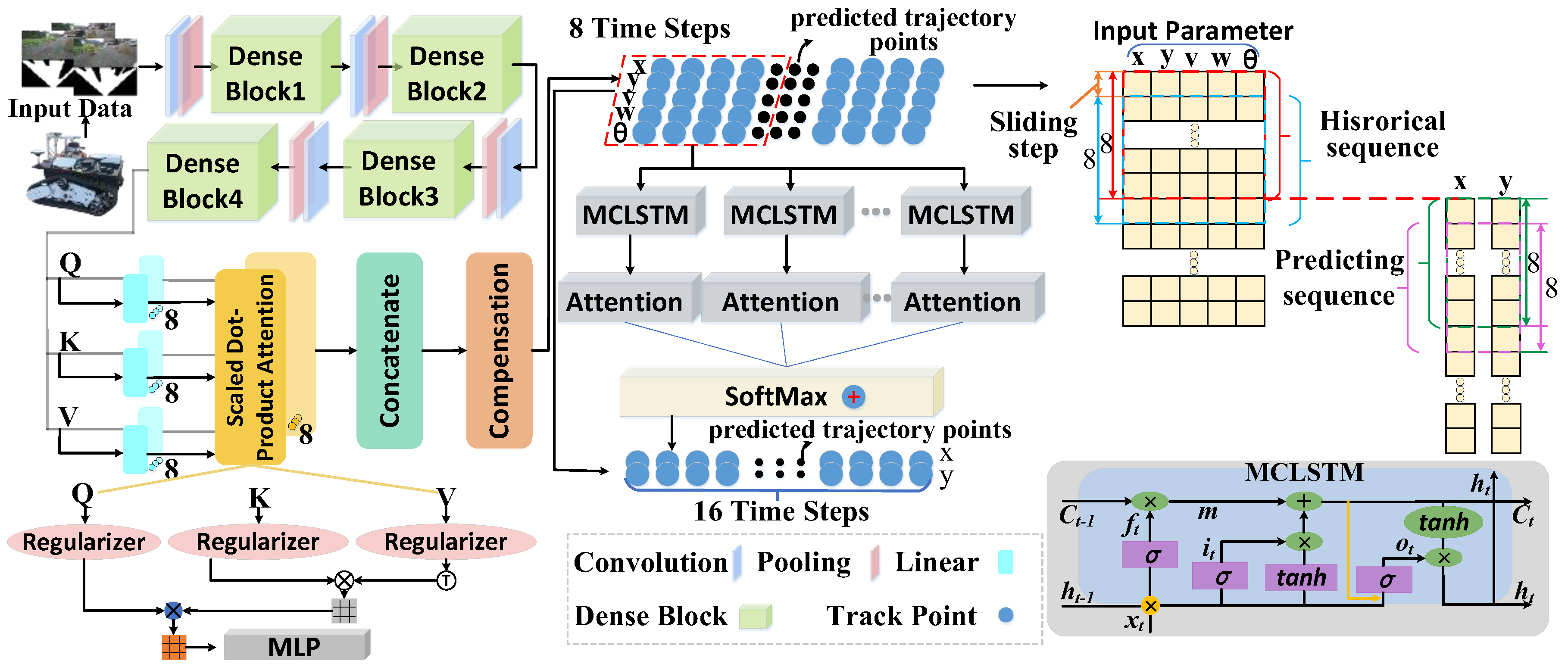
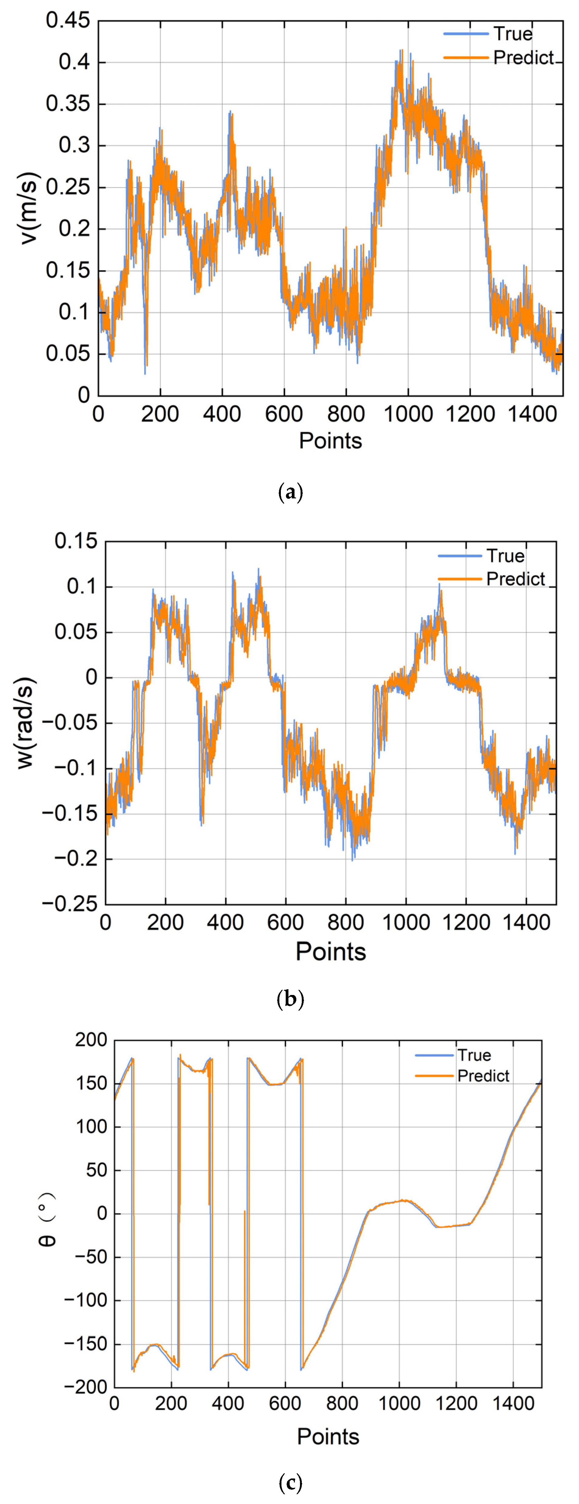
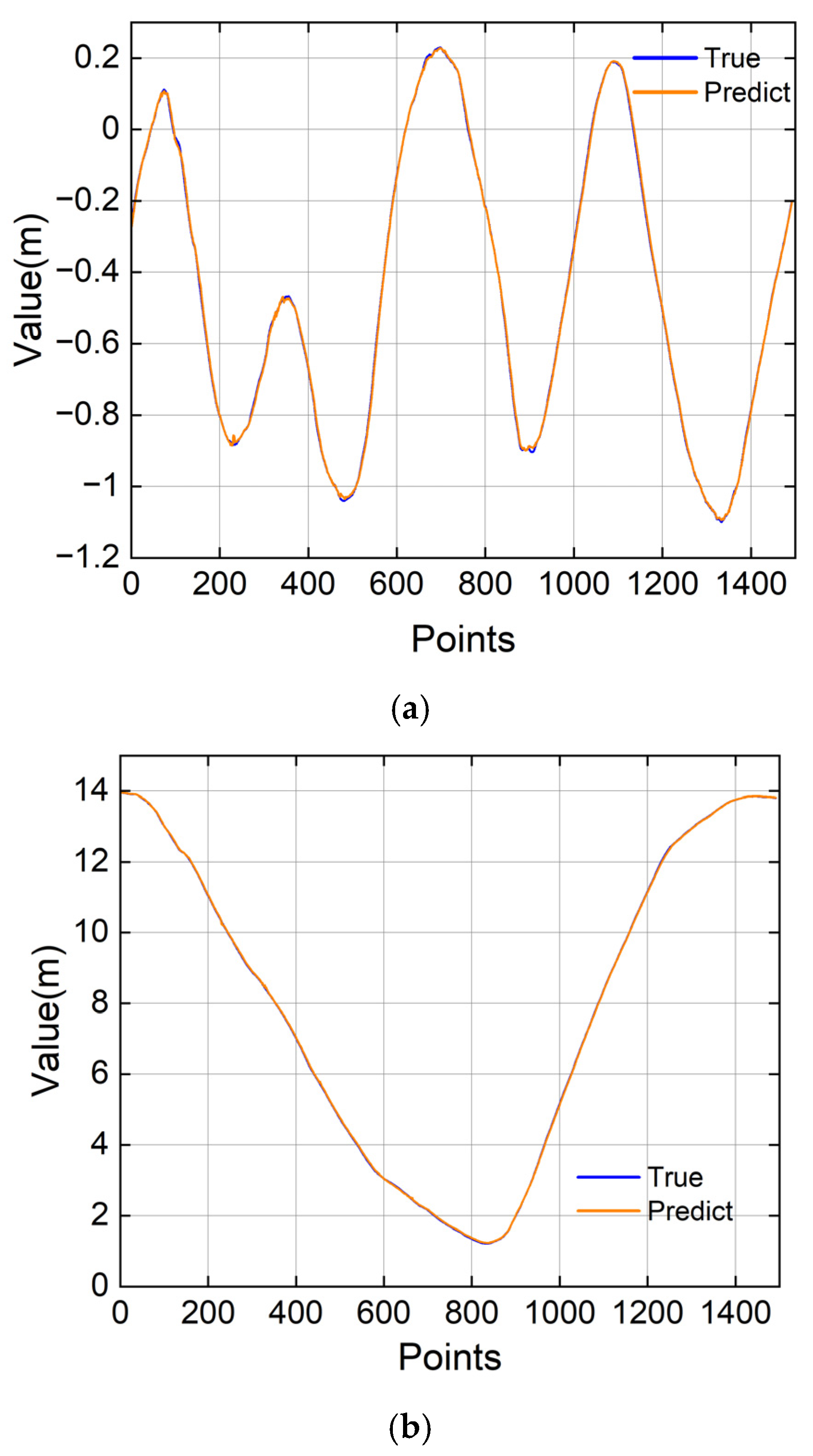
  • A two-stage trajectory-planning framework is proposed. In the first stage, the DAC network predicts trajectory points (x, y, v, w, and θ) over the next eight time steps. In the second stage, the MCLA network refines the x and y trajectory points by leveraging the temporal correlations in the first-stage outputs, generating a 16-step trajectory sequence.
  • A sliding multi-step prediction strategy is applied to generate long-horizon trajectory points, and vehicle dynamic parameters are incorporated as constraints to improve prediction accuracy.
The remainder of this paper is organized as follows. Section 2 reviews related work on trajectory planning. Section 3 presents the data acquisition process, data processing pipeline, analysis of manipulators’ proficiency levels, model architecture, training procedure, and key hyperparameter selection. Section 4 provides experimental validation of the proposed method, focusing on human-like trajectory performance and smoothness. Section 5 concludes this study.

2. Related Works

In recent years, trajectory-planning techniques have advanced significantly across various robotics domains. For instance, path planning under soft tissue deformation has been explored to address dynamic, non-rigid environments in surgical applications [30]. Cellular neural networks have been employed for optimal robot path planning [31] and real-time thermal modeling in robotic trajectory generation [32], demonstrating strong capabilities in real-time computation and spatial temporal reasoning. Moreover, metaheuristic optimization methods, such as the crossover recombination-based global-best brainstorm optimization algorithm, have proven effective in UAV path planning by enhancing global search and convergence efficiency [33]. Although these approaches are primarily applied in medical, aerial, or thermally constrained scenarios, their core principles—adaptability, real-time responsiveness, and global optimality—offer valuable insights for developing more robust and human-like trajectory-planning strategies in unstructured ground environments.
Most existing research on human-like steering trajectory planning focuses on functional design, while studies incorporating vehicle dynamic information for trajectory optimization remain limited. For example, Chen et al. developed a human-like steering planner for vehicle-turning scenarios in simulation and verified the feasibility of the generated trajectories under varying turning radii [34]. Yao et al. proposed a trajectory-planning method based on real-world driving data for lane-change intentions, generating parameterized lane-changing trajectories [35]. Wang et al. incorporated a polynomial trajectory generation model into a human–vehicle interaction system, forming a V2V framework for trajectory re-planning during lane changes; this approach enables reasonable trajectory generation under different lane-change intentions in simulated environments [36].
Trajectory optimization using dynamic information has also been investigated in hierarchical architectures. Ferguson et al. decomposed planning into three layers: task planning, behavior execution, and motion planning. Task planning determines the optimal route; behavior execution involves decisions such as following a vehicle or changing lanes; and motion planning generates trajectories that satisfy kinematic and dynamic constraints, forwarding the result to the control module for execution [37]. However, in this structure, the upper decision-making layer lacks detailed information, while the lower layer lacks the authority to reassess decisions, limiting its applicability in complex environments [38].
In this study, vehicle dynamic parameters (v, w, and θ) are used as constraints to generate an initial human-like trajectory based on environmental perception. The temporal relationships among the initially planned trajectory points are then utilized to perform a second-stage trajectory replanning for future long-horizon predictions.

3. Methods

Figure 1 shows the proposed vehicle human-like maneuvering trajectory-planning method with human maneuvering behaviors as the learning objective, which includes two parts.
Step 1: Human manipulation dataset acquisition and processing. The data collected by different manipulators during the human-maneuved vehicle obstacle avoidance driving in an environment with densely distributed obstacles were filtered, and the human manipulation dataset was constructed and used for network training.
Step 2: Network structure design and data training. A two-stage planning approach was adopted, using the DAC network for primary planning based on the environment space, followed by secondary planning using the MCLA network based on the time series of the trajectory points from the primary planning. Vehicle dynamic parameters were used as constraints to develop a long sequence of trajectories that better match human manipulation habits.
Specific methods for each component are discussed below.

3.1. Overview of the Proposed Framework

Fifteen participants were invited for testing, including eight male manipulators and seven female manipulators, ranging in age from 20 to 35 years. Variability was noted in the participants’ experience with fieldwork equipment manipulation.
Before the test, the operators were trained to ensure they were familiar with the data collection process and proficient in using the data collection equipment. Afterward, the testers were invited to maneuver the vehicle independently for data collection according to their own control habits, provided they were in good physical condition and the sensors did not interfere with their operation. Each tester drove at a speed of 1.2 km/h. The data collected during the test included point cloud data, image data, trajectory data, speed, angular velocity, heading angle, and other information related to the vehicle’s driving environment.
Figure 2 shows the data acquisition equipment. The tester manipulated the crawler model vehicle via wireless remote control to avoid densely distributed obstacles in the environment. The ZED2 camera collected images during driving and transmitted them to the display screen via 5G communication, allowing the tester to make decisions based on the scene displayed. A solid-state LiDAR was used to collect point cloud data from the environment for subsequent spatial analysis. Dynamic vehicle data, such as position, speed, angular velocity, and heading angle, were collected using an inertial navigation module in combination with fixed base stations via RTK technology, thereby improving the accuracy of the mobile navigation system. All sensing devices were connected to an NVIDIA jetson board. Prior to data collection, all sensors were initialized simultaneously to ensure timestamp consistency. Each operator collected 15 hours of data at a sampling frequency of 10 Hz in environments with varying obstacle densities.
To safely avoid obstacles, the vehicle continuously adjusted its heading and motion state in response to environmental changes. The forward and angular velocities at time t can be expressed as follows:
x ( t ) = 1 2 ( v l + v r ) cos θ d y ( t ) = 1 2 ( v l + v r ) sin θ d θ d ( t ) = - v l + v r D + 2 b ,
Transforming the preceding formula yields the following motion state equation:
W = x y θ = 1 2 cos θ d 1 2 sin θ d 1 D + 2 b 1 2 cos θ d 1 2 sin θ d 1 D + 2 b v l v r ,
where θd denotes the yaw angle, D represents the body width of the vehicle (0.74 m in this study), and b is the width of each track (0.15 m). vl and vr refer to the velocities of the left and right tracks, respectively. x and y denote the linear velocities in the x and y directions, while θ indicates the angular velocity. The driving posture of the vehicle is controlled by adjusting the relative velocities of the left and right tracks. The turning radius during motion is given by:
R = D + 2 b 2 · v l + v r v l v r ,

3.2. Human Manipulation Dataset Processing

(1)
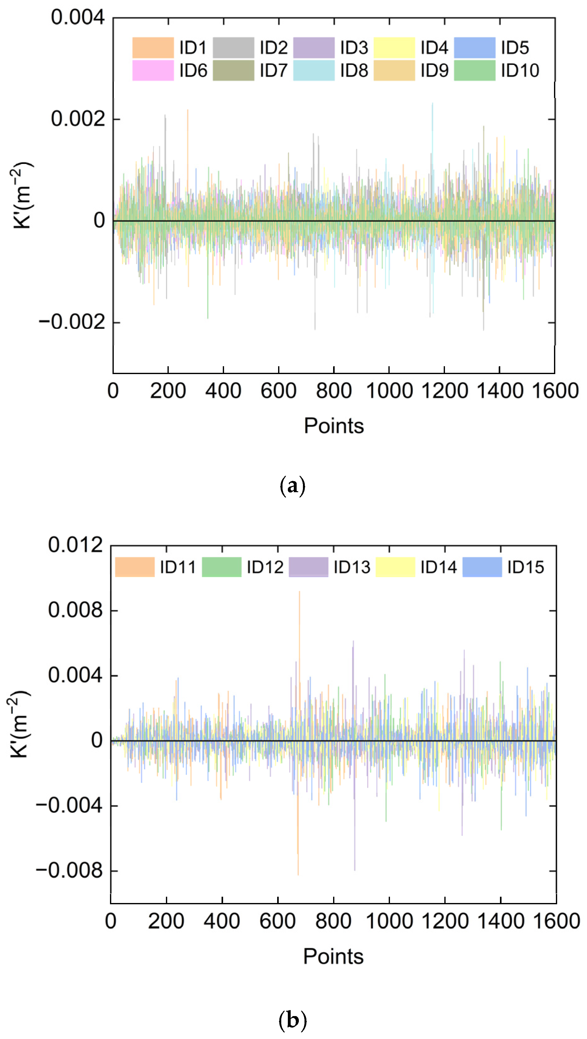
Human manipulation trajectory analysis
Because the differences in longitudinal displacement across testers are small, while transverse displacement more clearly reflects variation in maneuvering behavior, the similarity and smoothness of the data collected by different testers were analyzed based on transverse displacement.
First, the smoothness of the data collected by different testers was analyzed by calculating the curvature of the time series. A smaller curvature indicates smoother trajectories manipulated by the testers.
K = x ( 1 + x 2 ) 3 / 2 ,
K = x ( 1 + x 2 ) 3 / 2 3 x ( x ) 2 ( 1 + ( x ) 2 ) 5 / 2 ,
where x is the lateral displacement, K represents the curvature, and K′ is the derivative of the curvature. By analyzing the curvature and its derivative, data with better smoothness were selected and labeled as ID1–ID10 (skilled manipulators), while those with poorer smoothness were labeled as ID11–ID15 (unskilled manipulators). As shown in Figure 3, the curvature of the lateral displacement in data collected by skilled operators is primarily concentrated within a range of −0.002 to 0.002, whereas that from unskilled operators spans a broader range of −0.005 to 0.005. Similarly, Figure 4 illustrates that the curvature derivative for skilled operators falls within −0.001 to 0.001, while that for unskilled operators ranges from −0.004 to 0.004. These results indicate that the data collected by skilled operators demonstrate higher smoothness, enabling more stable and controlled obstacle-avoidance driving behavior.
Next, the similarity between the data collected by different manipulators was examined. Due to the different operating habits among testers, the lateral displacement deviations do not align directly in the time series. Therefore, Dynamic Time Warping (DTW) was used to measure the similarity between the datasets. DTW is a commonly used algorithm for comparing two time-series sequences that may vary in speed. It works by non-linearly aligning the sequences to minimize the cumulative distance between matched elements, even if the sequences differ in length or contain local time shifts. DTW stretches and compresses the sequences along the time axis to achieve local alignment and shape consistency. The algorithm then iteratively calculates and minimizes the cumulative distance between corresponding points in the two sequences. The formula is as follows:
D [ a ( i ) , b ( i ) ] = d [ a ( i ) , b ( i ) ] + min { D [ a ( i 1 ) , b ( j ) ] , D [ a ( i ) , b ( j 1 ) ] , D [ a ( i 1 ) , b ( j 1 ) ] } ,
where a and b are the sequence points in two different time series of A and B, respectively; d [ a ( i ) , b ( i ) ] is the distance between corresponding points; and D [ a ( i ) , b ( i ) ] is the cumulative distance of all matched points. The cumulative distance is converted into a similarity index within the range [0–1], where a value closer to 1 indicates a higher similarity between the two sequences. Specifically, one tester was randomly selected from the skilled group (labeled ID1), and the data collected by this tester were used as the benchmark. The similarity between the data from each subsequent tester and the ID1 data was then calculated. Table 1 shows differences in the data due to varying manipulation habits among skilled testers, but the overall similarity remains high. This high similarity indicates that skilled testers are more adept at avoiding obstacles in complex environments and can maneuver the vehicle more effectively. In contrast, the similarity between the data from unskilled testers and ID1 is relatively low, suggesting that unskilled testers are less capable of handing complex driving tasks and collect lower-quality data. The data collected from the screened skilled testers were used to construct the human maneuvering dataset.
(2)
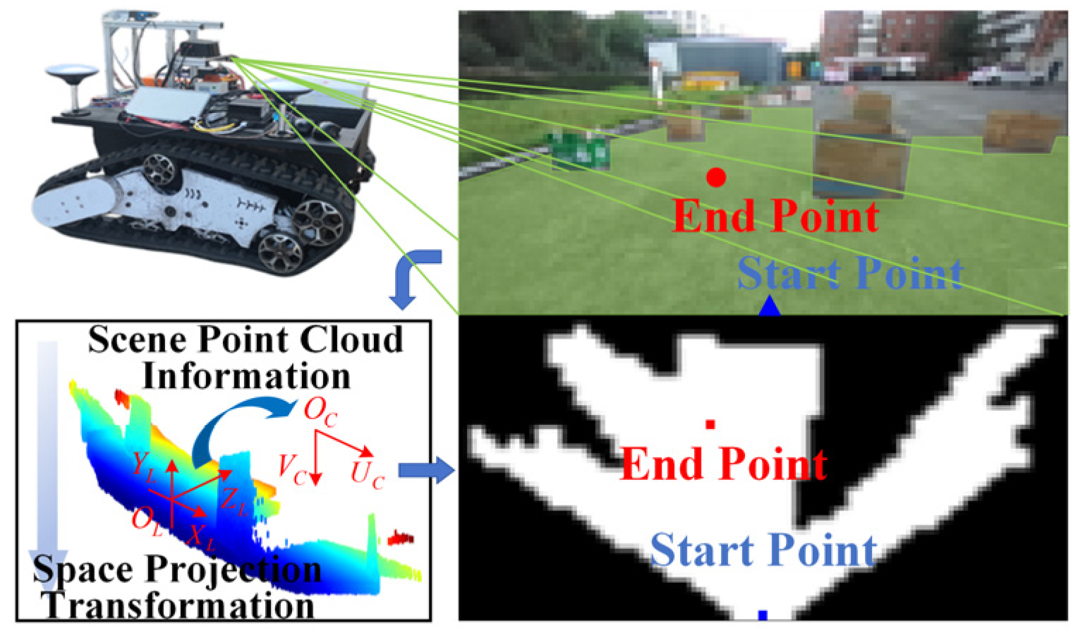
Driving space scene processing and analysis
During driving, testers chose routes with better passability based on their interpretation of the scene to to avoid obstacles. When guidance markers were present, testers were able to perceive and interpret the environment more accurately. Therefore, a feasible domain spatial map was overlaid on the original image as a visual reference, forming a composite 128 × 128 spatial representation, as shown in Figure 5. In this map, the blue point represents the starting position, the red point marks the target in the current scene, black pixels indicate non-drivable areas, and the white pixels indicate drivable areas. The feasible domain map is generated via spatial projection based on height gradients from the point cloud. The coordinate system is transformed from the LiDAR frame to the pixel-based feasible domain frame to obtain a 2D spatial map. The coordinate transformation formula is as follows:
λ u i v i 1 = M R T x l y l z l 1 ,
where xl, yl, zl are the point cloud coordinates in the LiDAR system; λ is the scale factor; ui and vi are the point cloud coordinates in the pixel coordinate system; M denotes the camera internal reference; and R and T are the rotation matrix and translation vector between the camera and the LiDAR. The equation only performs spatial projection from the LiDAR coordinate system to the pixel coordinate system.
The spatial pictures processed above were grouped with the collected x, y, v, w, and θ data. Each image corresponds to eight time-step trajectory points, which were used to train the DAC network to map future trajectory points over the next eight time steps based on spatial location relationships. This portion of the dataset was recorded as data1. Subsequently, the captured human manipulation trajectories were organized sequentially for training the MCLA network. This portion of the dataset was recorded as data2. Finally, based on the temporal relationships between trajectory points predicted by the DAC network, the MCLA network was used to further plan the trajectory points for the next eight time steps. A total of 12,558 data groups were generated after processing.

3.3. Design of Network Structure for Two-Stage Trajectory Planning

Based on the spatial characteristics and the time-series relationship of the trajectory points, a two-stage planning approach was used to plan the future long-horizon trajectory. The specific model is shown in Figure 6.
First, part of the DenseNet network structure was used to extract spatial features from 128 × 128 images. As DenseNet extensively employs batch normalization and cross-layer connectivity, it helps mitigate gradient vanishing and model degradation problems. The structure mainly consists of transition modules and dense connection modules. Assuming L convolutional layers in each dense connection module, the output feature map from the Lth convolutional layer is concatenated along the channel dimension with the output feature maps from the 1st to L-1th layers, with all feature maps having the same spatial size. The derivation formula is as follows:
A L = S L ( [ S 1 , S i , , S L 1 ] ) ,
where Ai represents the feature map output from the ith convolutional layer, and Si denotes the computation of a series of nonlinear transformation functions such as batch normalization, activation functions, and convolution. Since feature reuse may result in computational overload in deeper layers, each module was first processed with a 1 × 1 convolutional kernel to reduce channel dimensionality before further convolution. In the transition modules, features were compressed using a combination of batch normalization, ReLU activation, 1 × 1 convolutional layer, and pooling layers, which helped reduce the overall computational load of the model.
Next, the correlation between the features extracted in the previous section was enhanced using multi-head attention, and the output trajectory points were improved by introducing an error compensation layer. The features were mapped into three spaces: keys (K), queries (Q) and values (V),with the features in K, Q, and V following the same distribution. The similarity between features in the K and Q spaces was then computed to enhance the features in the V space. The dot product attention and multi-head attention for each layer were calculated as follows:
A t t e n t i o n ( q , k , v ) = s o f t max ( q k T d ) v ,
M u l t i H e a d ( q , k , v ) = f c ( c o n c a t ( { A t t e n t i o n i ( q , k , v ) } i = 1 H ) ) ,
where query matrix q, key matrix k, and value matrix v are the three inputs. d is the dimension of k, the softmax function is used to obtain the weights of the values, and fc() denotes a fully connected layer that integrates all head outputs. Each attention layer also contains a multilayer perceptron (MLP) for further extraction of attention features expressed as:
A T T ( q , k , v ) = M L P ( M u l t i H e a d ( q , k , v ) ) ,
where ATT is the output of the attention layer. After the attention layer, an error compensation structure was added to improve the accuracy of the predicted trajectory points. The computation is as follows:
Δ a = t 0 p 0 Δ b = Δ a · w i + b i p l = p i + Δ b ,
where t0 is the first value in the sequence, p0 is the first sequence point, Δa is the difference between the true value and predicted points at the first time step, wi and bi are trainable parameters, pi is the predicted point, and pl is the compensated prediction point.
Finally, to capture the temporal correlation of the trajectory points predicted in the previous step, a sliding prediction method was applied using the LSTM network to replan trajectory points over the next eight time steps. An attention mechanism was incorporated into the final hidden layer to improve prediction accuracy. The x, y, v, w, and θ variables predicted for the previous eight time steps were used to forecast the x and y trajectory points of the subsequent eight time steps. The LSTM neuron consists of input gates it, forget gates ft, and output gates ot, which work together with the memory cells ct to collaboratively learn from the multivariate input data. This input data are denoted as Γ R L × K , where L is the number of temporal sampling instances, and K is the number of variables. After the LSTM cell outputs a vector ht, the computation is expressed as follows:
i t = σ ( W Γ i Γ t × W h i h t 1 + b i ) ,
f t = σ [ ( W Γ f + Δ W ) Γ t × ( W h f + Δ W ) h t 1 + ( b f + Δ b ) ] ,
c t = f t c t 1 + i t tanh ( W Γ c Γ t + W h c h t 1 + b c ) ,
o t = σ ( W Γ o Γ t + W h o h t 1 + b o ) ,
h t = o t tanh ( c t ) ,
where is the element-wise product, σ ( x ) = 1 / ( 1 + e x ) denotes the sigmoid activation function, W u v ( u , v { Γ , i , f , c , h , o } ) is the weight matrix, and b u ( u { i , f , c , o } ) is the bias vector. In the output vector, the cosine similarity ei with the previous hidden layer is computed. Softmax is then applied to calculate the weight of each input sample based on the similarity, thereby producting the final predicted trajectory points using the following formula:
e i = h · h h h ,
h t = o t tanh ( c t ) ,
where h is output vector of the current hidden layer, h is the output vector of the previous hidden layer, and is the normalization factor (norm).

3.4. Model Training and Evaluation

The data1 and data2 datasets were used to train the DAC network and MCLA network, respectively. The predicted outputs of the DAC network were then used for secondary planning to generate long-horizon trajectory points over the next 16 time steps. During training, the human manipulation dataset was divided into training, validation, and testing sets in a ratio of 8:1:1, and all the data were normalized. The network was trained using the mean square error (MSE) as the loss function, defined as follows:
L o s s = M S E = 1 N i = 1 N ( r i r ) 2 ,
where N is the number of training samples, ri is the actual trajectory coordinate of the skilled tester, and r i is the predicted trajectory coordinate. The objective of iterative training is to minimize the value of Loss. Hyperparameters were selected based on commonly used configurations in related studies. To prevent overfitting, a learning rate decay factor was introduced. The LSTM network was configured with two layers, each containing 196 hidden units, to balance model capacity and computational cost. A dropout layer was also used to improve the generalization ability of the model. Bayesian optimization was applied to determine the optimal hyperparameter configuration, as shown in Table 2.

4. Experimentation and Analysis

To validate the effectiveness of the proposed method, the accuracy and smoothness of the planned trajectory were analyzed through ablation experiments and comparison with other methods in the field of human-like trajectory planning. Trajectory accuracy was evaluated by the error between planned and actual trajectories, including the root mean square error (RMSE) and mean average error (MAE). Trajectory smoothness was assessed using the standard deviation of the angular acceleration and the curvature.

4.1. Ablation Experiment

In the experiments, we used data from new scenarios to conduct a series of tests to compare the effects of each component in the proposed method and evaluate its generalization ability and prediction accuracy. Error, RMSE, and MAE were used as evaluation metrics. Proposed refers to the method presented in this study; D represents the DenseNet-only approach; DMA denotes the combination of DenseNet and multi-head attention; and P-L refers to the second prediction stage of the proposed method using a standard (unimproved) LSTM network.
Figure 7a shows that, in terms of prediction error in the x and y directions, the D method alone yields larger errors. When multi-head attention is introduced, the prediction accuracy improves by a factor of 1, indicating that multi-head attention can effectively enhance the mapping capacity of DenseNet. Figure 7b shows that when temporal sequences between trajectory points are considered, the trajectory prediction accuracy improves by a factor of 5, highlighting the significant impact of temporal correlation. After introducing the attention mechanism into the hidden layer of the LSTM network, the prediction accuracy is further improved, demonstrating the effectiveness of attention in the LSTM weighting layer. The error in the x direction between the trajectory predicted by the proposed method and that generated by human operation falls within the range of −0.02 m to 0.02 m, indicating that the proposed method is capable of generating trajectories comparable to human operation in environments with complex, distributed obstacles.
Figure 8 shows that the proposed method achieves a good fit between the predicted and actual kinematic parameters in the first stage, indicating it can provide reliable constraints for second-stage predictions. After using the first-stage trajectory points to predict the next eight time steps, Figure 9 shows that the predicted and actual trajectories in the x and y directions almost completely overlap. Table 3 and Table 4 show that RMSE and MAE reach their minimum values under the proposed method, suggesting that the model successfully learns human manipulation habits.

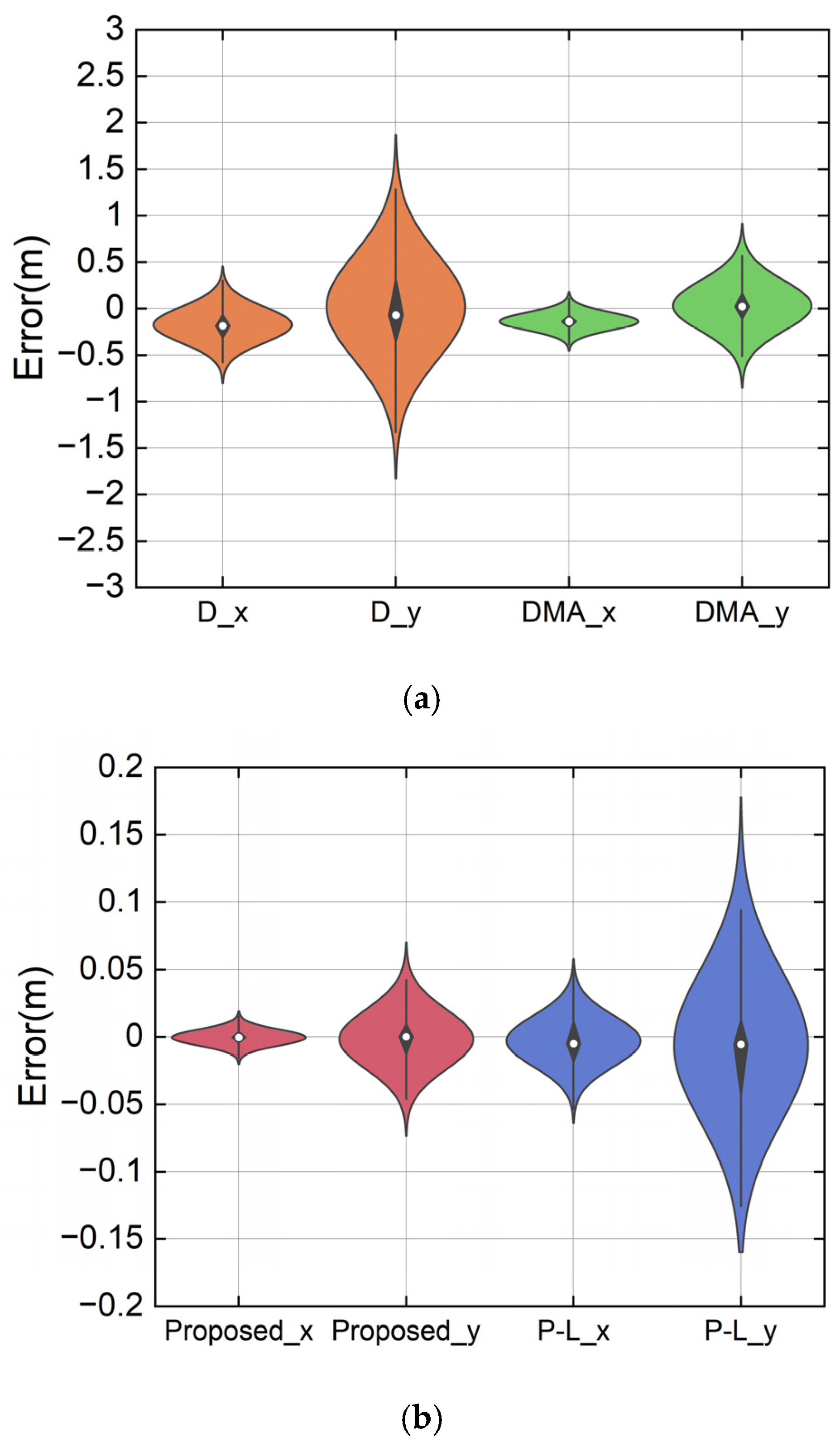
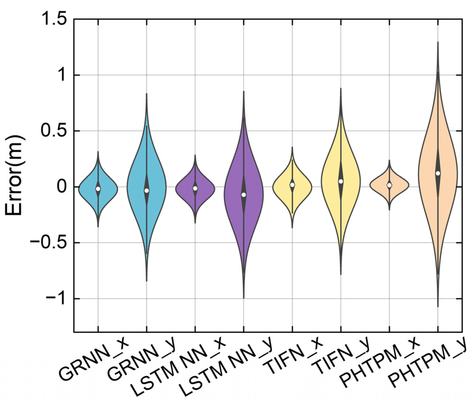
4.2. Comparison Experiment

To further verify the effectiveness of the proposed method, it was compared with four representative approaches in human-like driving trajectory planning: (a) the GRNN model was proposed in [39], which leverages the nonlinear approximation capability of radial basis function networks to learn the behavioral characteristics of skilled drivers; (b) the long short-term memory(LSTM) neural network model presented in [40], designed to learn the driving behavior of skilled drivers on curves; (c) the temporal information fusion network introduced in [41], which captures the correlation between driving behavior and the external environment using a lightweight end-to-end structure; (d) the PHTPM model proposed in [26], which learns human driving characteristics through behavioral mechanisms to generate human-like planned trajectories. A comparison between Figure 7b and Figure 10 shows that the proposed method significantly improves trajectory prediction accuracy. Table 3 and Table 4 indicate that it achieves the lowest RMSE and MAE between the predicted and actual values, demonstrating its effectiveness in human-like trajectory planning across spatially distributed scenarios. The generated trajectories closely resemble human manipulation patterns.

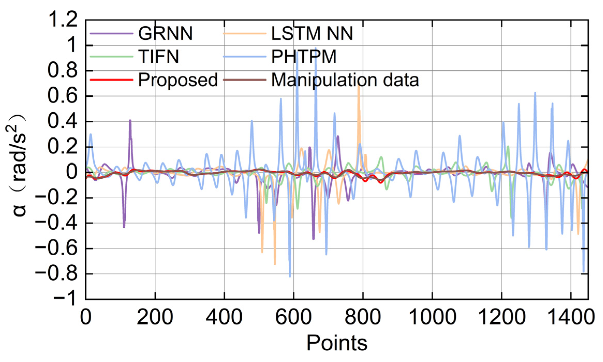
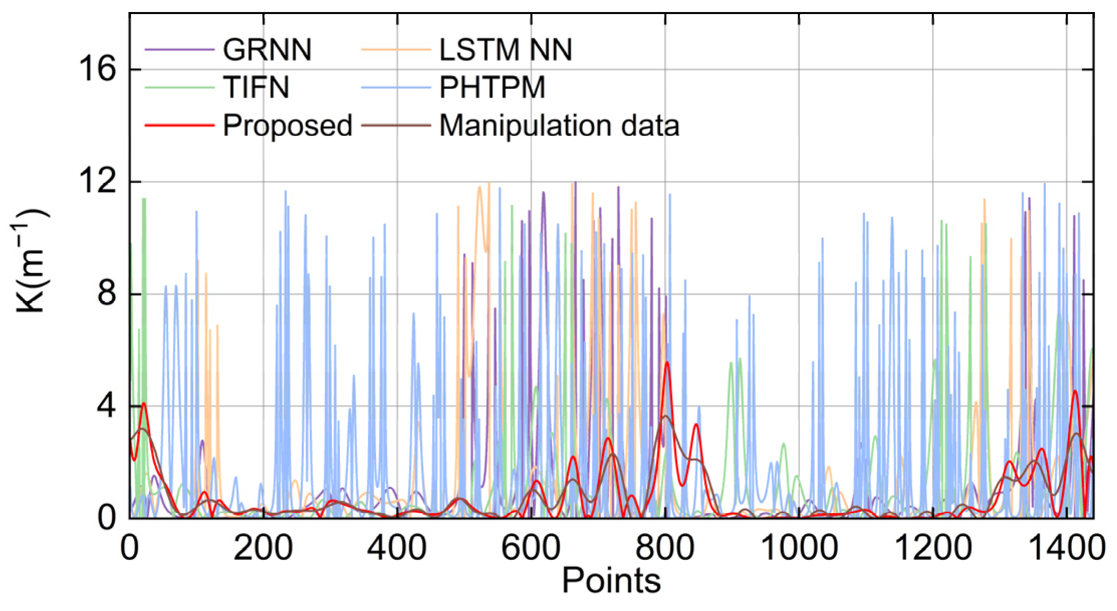
4.3. Evaluation of Trajectory Smoothness

As the planned trajectory is time-ordered, the continuity of angular acceleration variation and trajectory curvature reflects the smoothness of the trajectory. Therefore, in this study, the standard deviation (SD) of angular acceleration and curvature is used as the evaluation metric for trajectory smoothness, and the SD of the curvature is normalized for better observation.
S D = 1 n i = 1 n ( P i P i ) 2 ,
K = y ( 1 + y 2 ) 3 / 2 ,
where P i is the predicted trajectory value, Pi is the mean of the predicted trajectory, y is the vertical coordinate, and K is the curvature. As shown in Figure 11, the angular acceleration of the trajectory planned by the proposed method is significantly lower than that of the comparison methods, indicating a lower oscillation frequency that more closely resembles the trajectory of human operation. Figure 12 shows that the trajectory generated by the proposed method exhibits stronger continuity in curvature fluctuations and higher similarity to human-operated trajectories, suggesting better trajectory continuity. Table 5 presents a comparison of the standard deviations of the two metrics. It is evident that the proposed method achieves the smallest SD values in both angular acceleration and curvature, with minimal deviation from the values observed in human-operated trajectories. These results demonstrate that the proposed method generates smoother trajectories, contributing to improved safety, stability, and robustness in trajectory tracking, while reducing the risk of slippage. Moreover, since the method does not rely on constructing a kinematic vehicle model, it is relatively easy to transfer and deploy across different vehicle platforms.

5. Summary

This study proposes a method for planning trajectory points over future long time steps by incorporating human maneuvering behavior under vehicle dynamics constraints. After analyzing the similarity of the data in terms of lateral displacement and the degree of curvature variation, samples with better smoothness were filtered to construct a human manipulation behavior dataset for training and testing the trajectory-planning network. The dynamic information was then introduced as a constraint, and a two-stage human-like planning network was designed to sequentially predict trajectory points over a long time horizon. Experimental comparisons with multiple existing methods show that the proposed method achieves lower RMSE and MAE between the planned and actual trajectories, indicating a better ability to capture human manipulation characteristics. In addition, the SD of angular acceleration and curvature demonstrates that the planned trajectories generated by the proposed method are smoother than those of other approaches. Therefore, the proposed approach not only provides sufficient decision time for dynamic obstacle avoidance but also contributes to enhancing the overall driving performance of autonomous vehicles.

Author Contributions

Conceptualization, H.X.; methodology, H.X.; software, H.X.; validation, H.X.; formal analysis, H.X.; investigation, H.X.; resources, H.Z.; data curation, H.X.; writing—original draft preparation, H.X.; writing—review and editing, H.X.; visualization, G.Z.; supervision, H.Z.; project administration, G.Z. and H.Z.; funding acquisition, H.Z. All authors have read and agreed to the published version of the manuscript.

Funding

This work was supported by the Science and Technology Development Project of Jilin Province, China [grant number: 20240302057GX], and the Science and Technology Development Project of Changchun, China [grant number: 23GNYZ31].

Data Availability Statement

The original contributions presented in the study are included in the article; further inquiries can be directed to the corresponding author.

Conflicts of Interest

The authors declare no conflicts of interest.

References

  1. Jo, K.; Kim, J.; Kim, D.; Jang, C. Development of autonomous car—Part I: Distributed system architecture and development process. IEEE Trans. Ind. Electron. 2014, 61, 7131–7140. [Google Scholar] [CrossRef]
  2. Sadat, A.; Ren, M.; Pokrovsky, A.; Lin, Y.-C. Jointly learnable behavior and trajectory planning for self-driving vehicles. In Proceedings of the 2019 IEEE/RSJ International Conference on Intelligent Robots and Systems (IROS), Macau, China, 3–8 November 2019; IEEE: New York, NY, USA, 2019; pp. 3949–3956. [Google Scholar]
  3. Huang, Z.; Mo, X.; Lv, C. Multi-modal motion prediction with transformer-based neural network for autonomous driving. In Proceedings of the 2022 International Conference on Robotics and Automation (ICRA), Philadelphia, PA, USA, 23–27 May 2022; IEEE: New York, NY, USA, 2022; pp. 2605–2611. [Google Scholar]
  4. Xu, D.; Ding, Z.; He, X.; Zhao, H.; Moze, M.; Aioun, F.; Guillemard, F. Learning from naturalistic driving data for human-like autonomous highway driving. IEEE Trans. Intell. Transp. Syst. 2020, 22, 7341–7354. [Google Scholar] [CrossRef]
  5. Chen, S.; Chen, Y.; Zhang, S.; Zheng, N.-N. A novel integrated simulation and testing platform for self-driving cars with hardware in the loop. IEEE Trans. Intell. Veh. 2019, 4, 425–436. [Google Scholar] [CrossRef]
  6. Li, Y.; Wei, W.; Gao, Y.; Wang, D.; Fan, Z. PQ-RRT*: An improved path planning algorithm for mobile robots. Expert Syst. Appl. 2020, 152, 113425. [Google Scholar] [CrossRef]
  7. Tang, J.; Wang, Y.; Hao, W.; Liu, F.; Huang, H.; Wang, Y. A Mixed Path Size Logit-Based Taxi Customer-Search Model Considering Spatio-Temporal Factors in Route Choice. IEEE Trans. Intell. Transp. Syst. 2020, 21, 1347–1358. [Google Scholar] [CrossRef]
  8. Zhang, S.; Wang, R.; Jian, Z.; Zhan, W.; Zheng, N.; Tomizuka, M. Clothoid-Based Reference Path Reconstruction for HD Map Generation. IEEE Trans. Intell. Transp. Syst. 2023, 25, 587–601. [Google Scholar] [CrossRef]
  9. Noh, S. Decision-making framework for autonomous driving at road intersections: Safeguarding against collision, overly conservative behavior, and violation vehicles. IEEE Trans. Ind. Electron. 2018, 66, 3275–3286. [Google Scholar] [CrossRef]
  10. Schwarting, W.; Alonso-Mora, J.; Rus, D. Planning and decision-making for autonomous vehicles. Annu. Rev. Control. Robot. Auton. Syst. 2018, 1, 187–210. [Google Scholar] [CrossRef]
  11. Yang, W.; Zheng, L.; Li, Y.; Ren, Y.; Xiong, Z. Automated highway driving decision considering driver characteristics. IEEE Trans. Intell. Transp. Syst. 2019, 21, 2350–2359. [Google Scholar] [CrossRef]
  12. Xu, X.; Zuo, L.; Li, X.; Qian, L.; Ren, J.; Sun, Z. A Reinforcement Learning Approach to Autonomous Decision Making of Intelligent Vehicles on Highways. IEEE Trans. Syst. Man Cybern. Syst. 2020, 50, 3884–3897. [Google Scholar] [CrossRef]
  13. Hoel, C.-J.; Driggs-Campbell, K.; Wolff, K.; Laine, L.; Kochenderfer, M.J. Combining Planning and Deep Reinforcement Learning in Tactical Decision Making for Autonomous Driving. IEEE Trans. Intell. Veh. 2020, 5, 294–305. [Google Scholar] [CrossRef]
  14. Bansal, M.; Krizhevsky, A.; Ogale, A. ChauffeurNet: Learning to drive by imitating the best and synthesizing the worst. In Proceedings of the Robotics: Science and Systems 2019, Freiburg im Breisgau, Germany, 22–26 June 2019; pp. 1–10. [Google Scholar]
  15. Chitta, K.; Prakash, A.; Geiger, A. Neat: Neural attention fields for end-to-end autonomous driving. In Proceedings of the IEEE/CVF International Conference on Computer Vision, Montreal, BC, Canada, 11–17 October 2021; pp. 15793–15803. [Google Scholar]
  16. Zhu, Z.; Zhao, H. A Survey of Deep RL and IL for Autonomous Driving Policy Learning. IEEE Trans. Intell. Transp. Syst. 2022, 23, 14043–14065. [Google Scholar] [CrossRef]
  17. Kiran, B.R.; Sobh, I.; Talpaert, V.; Mannion, P.; Al Sallab, A.A.; Yogamani, S.; Perez, P. Deep Reinforcement Learning for Autonomous Driving: A Survey. IEEE Trans. Intell. Transp. Syst. 2022, 23, 4909–4926. [Google Scholar] [CrossRef]
  18. Wu, J.; Huang, Z.; Lv, C. Uncertainty-Aware Model-Based Reinforcement Learning: Methodology and Application in Autonomous Driving. IEEE Trans. Intell. Veh. 2023, 8, 194–203. [Google Scholar] [CrossRef]
  19. Wu, J.; Huang, Z.; Hu, Z.; Lv, C. Toward human-in-the-loop AI: Enhancing deep reinforcement learning via real-time human guidance for autonomous driving. Engineering 2023, 21, 75–91. [Google Scholar] [CrossRef]
  20. Wu, J.; Huang, Z.; Huang, W.; Lv, C. Prioritized experience-based reinforcement learning with human guidance for autonomous driving. IEEE Trans. Neural Netw. Learn. Syst. 2022, 35, 855–869. [Google Scholar] [CrossRef] [PubMed]
  21. Rosbach, S.; James, V.; Großjohann, S.; Homoceanu, S.; Roth, S. Driving with Style: Inverse Reinforcement Learning in General-Purpose Planning for Automated Driving. In Proceedings of the 2019 IEEE/RSJ International Conference on Intelligent Robots and Systems (IROS), Macau, China, 3–8 November 2019; pp. 2658–2665. [Google Scholar]
  22. Nakamura, Y.; Yamane, K.; Fujita, Y.; Suzuki, I. Somatosensory computation for man-machine interface from motion-capture data and musculoskeletal human model. IEEE Trans. Robot. 2005, 21, 58–66. [Google Scholar] [CrossRef]
  23. Wang, W.; Li, R.; Diekel, Z.M.; Chen, Y.; Zhang, Z.; Jia, Y. Controlling Object Hand-Over in Human–Robot Collaboration Via Natural Wearable Sensing. IEEE Trans. Hum.-Mach. Syst. 2019, 49, 59–71. [Google Scholar] [CrossRef]
  24. Rodriguez, M.; Orrite, C.; Medrano, C.; Makris, D. One-Shot Learning of Human Activity With an MAP Adapted GMM and Simplex-HMM. IEEE Trans. Cybern. 2017, 47, 1769–1780. [Google Scholar] [CrossRef]
  25. Ijspeert, A.J.; Nakanishi, J.; Hoffmann, H.; Pastor, P.; Schaal, S. Dynamical movement primitives: Learning attractor models for motor behaviors. Neural Comput. 2013, 25, 328–373. [Google Scholar] [CrossRef]
  26. Zhao, J.; Song, D.; Zhu, B.; Sun, Z.; Han, J.; Sun, Y. A Human-Like Trajectory Planning Method on a Curve Based on the Driver Preview Mechanism. IEEE Trans. Intell. Transp. Syst. 2023, 24, 11682–11698. [Google Scholar] [CrossRef]
  27. Li, G.; Yang, L.; Li, S.; Luo, X.; Qu, X.; Green, P. Human-like decision making of artificial drivers in intelligent transportation systems: An end-to-end driving behavior prediction approach. IEEE Intell. Transp. Syst. Mag. 2022, 14, 188–205. [Google Scholar] [CrossRef]
  28. Behera, A.; Wharton, Z.; Keidel, A.; Debnath, B. Deep CNN, Body Pose, and Body-Object Interaction Features for Drivers’ Activity Monitoring. IEEE Trans. Intell. Transp. Syst. 2022, 23, 2874–2881. [Google Scholar] [CrossRef]
  29. Santhosh, K.K.; Dogra, D.P.; Roy, P.P.; Mitra, A. Vehicular Trajectory Classification and Traffic Anomaly Detection in Videos Using a Hybrid CNN-VAE Architecture. IEEE Trans. Intell. Transp. Syst. 2022, 23, 11891–11902. [Google Scholar] [CrossRef]
  30. Bahwini, T.; Zhong, Y.; Gu, C. Path planning in the presence of soft tissue deformation. Int. J. Interact. Des. Manuf. (IJIDeM) 2019, 13, 1603–1616. [Google Scholar] [CrossRef]
  31. Zhong, Y.; Shirinzadeh, B.; Yuan, X. Optimal robot path planning with cellular neural network. In Advanced Engineering and Computational Methodologies for Intelligent Mechatronics and Robotics; IGI Global: Hershey, PA, USA, 2013; pp. 19–38. [Google Scholar]
  32. Hills, J.; Zhong, Y. Cellular neural network-based thermal modelling for real-time robotic path planning. Int. J. Agil. Syst. Manag. 2014, 20, 261–281. [Google Scholar] [CrossRef]
  33. Zhou, Q.; Gao, S.; Qu, B.; Gao, X.; Zhong, Y. Crossover recombination-based global-best brain storm optimization algorithm for uav path planning. Proc. Rom. Acad. Ser. A-Math. Phys. Tech. Sci. Inf. Sci. 2022, 23, 207–216. [Google Scholar]
  34. You, F.; Zhang, R.; Lie, G.; Wang, H.; Wen, H.; Xu, J. Trajectory planning and tracking control for autonomous lane change maneuver based on the cooperative vehicle infrastructure system. Expert Syst. Appl. 2015, 42, 5932–5946. [Google Scholar] [CrossRef]
  35. Dubey, P.K.; Singh, B.; Kumar, V.; Singh, D. A Novel Approach for Comparative Analysis of Distributed Generations and Electric Vehicles in Distribution Systems. Electr. Eng. 2022, 106, 2371–2390. [Google Scholar] [CrossRef]
  36. Huang, Y.; Wang, H.; Khajepour, A.; Ding, H.; Yuan, K.; Qin, Y. A Novel Local Motion Planning Framework for Autonomous Vehicles Based on Resistance Network and Model Predictive Control. IEEE Trans. Veh. Technol. 2020, 69, 55–66. [Google Scholar] [CrossRef]
  37. Ferguson, D.; Howard, T.M.; Likhachev, M. Motion planning in urban environments. J. Field Robot. 2008, 25, 939–960. [Google Scholar] [CrossRef]
  38. Wei, J.; Snider, J.M.; Gu, T.; Dolan, J.M.; Litkouhi, B. A behavioral planning framework for autonomous driving. In Proceedings of the IEEE Symposium on Intelligent Vehicle, Cluj, Romania, 2–5 June 2024; pp. 458–464. [Google Scholar]
  39. Li, A.; Jiang, H.; Li, Z.; Zhou, J.; Zhou, X. Human-like trajectory planning on curved road: Learning from human drivers. IEEE Trans. Intell. Transp. Syst. 2020, 21, 3388–3397. [Google Scholar] [CrossRef]
  40. Li, A.; Jiang, H.; Zhou, J.; Zhou, X. Learning human-like trajectory planning on urban two-lane curved roads from experienced drivers. IEEE Access 2019, 7, 65828–65838. [Google Scholar] [CrossRef]
  41. Guo, C.; Liu, H.; Chen, J.; Ma, H. Temporal Information Fusion Network for Driving Behavior Prediction. IEEE Trans. Intell. Transp. Syst. 2023, 24, 9415–9424. [Google Scholar] [CrossRef]
Figure 1. Flow and structure of the proposed method.
Vehicles 07 00063 g001
Figure 2. Hardware device composition.
Vehicles 07 00063 g002
Figure 3. Comparison of lateral displacement curvature of data: (a) transverse displacement curvature of data collected by skilled testers; (b) curvature of lateral displacement of data collected by unskilled testers.
Vehicles 07 00063 g003aVehicles 07 00063 g003b
Figure 4. Comparison of the curvature derivatives of lateral displacement: (a) the derivative of the curvature of lateral displacement in the data collected by skilled operators; (b) the derivative of the curvature of lateral displacement in the data collected by unskilled operators.
Vehicles 07 00063 g004
Figure 5. Real scenario and extracted spatial map of the feasible domain, where XL-YL-ZL is the LiDAR coordinate system, and UC-OC-VC is the feasible domain coordinate system.
Vehicles 07 00063 g005
Figure 6. Two-stage trajectory-planning network structure. Abbreviations: MCLSTM refers to Multiplication Cell-State LSTM; Q, K, and V represent the Query, Key, and Value components from the attention mechanism; MLP denotes Multi-Layer Perceptron; SoftMax is the SoftMax activation function; x, y, w, and θ indicate position and orientation parameters; it, ft, ot, m, Ct, and h refer to LSTM internal gates and states, including input gate, forget gate, output gate, memory, cell state, and hidden state.
Vehicles 07 00063 g006
Figure 7. Comparison of the output values of each method in the x and y directions with the error of the true values: (a) comparison of the error between the output values and the true values in x and y directions for D and DMA methods; (b) comparison of the error between the output values and the true values in the x and y directions for the proposed and P-L methods.
Vehicles 07 00063 g007
Figure 8. First-stage kinetic parameter fitting curves: (a) velocity fitting curve; (b) angular velocity fitting curve; (c) heading angle fitting curves.
Vehicles 07 00063 g008
Figure 9. Final trajectory output fit: (a) fit in the x direction of the test set; (b) fit in y direction of the test set.
Vehicles 07 00063 g009
Figure 10. Comparison method x, y direction output value and real value error.
Vehicles 07 00063 g010
Figure 11. Comparison of transverse pendulum angular acceleration for planned trajectories.
Vehicles 07 00063 g011
Figure 12. Comparison of curvature continuity of planning trajectories.
Vehicles 07 00063 g012
Table 1. Similarity analysis of data collected by each tester.
Skilled TesterID2ID3ID4ID5ID6ID7ID8ID9ID10
Similarity0.9410.950.9660.9710.9690.9570.9540.9730.977
Unskilled testerID11ID12ID13ID14ID15////
Similarity0.8210.8730.8150.8520.796////
Table 2. Hyperparameters of proposed model.
HyperparameterCandidate ValuesValue
Initial learning rate[0.001, 0.005, 0.01, 0.02]0.01
Learning rate drop out period[50, 100, 150, 200]100
Learning rate drop out factor[0.1, 0.2, 0.5, 0.8]0.1
Batch size[200, 300, 400, 500]300
Epoch number[300, 500, 800, 1000]500
numLayers of lstm[1, 2, 3, 4]2
numHiddenUnits[128, 160, 196, 256]196
dropoutLayer[0.1, 0.2, 0.3, 0.5]0.1
Table 3. Root mean square error for each comparison method.
RMSE
(Proposed)
RMSE
(P-L)
RMSE
(D)
RMSE
(DMA)
RMSE
(GRNN)
RMSE
(LSTM NN)
RMSE
(TIFN)
RMSE
(PHTPM)
x0.0060.0190.2590.1680.1050.0950.110.070
y0.0220.0570.5680.2720.2570.2930.2590.381
Table 4. Mean absolute error for each comparison method.
MAE
(Proposed)
MAE
(P-L)
MAE
(D)
MAE
(DMA)
MAE
(GRNN)
MAE
(LSTM NN)
MAE
(TIFN)
MAE
(PHTPM)
x0.0050.0160.220.1430.0830.0770.0840.054
y0.0160.0410.4250.190.1930.2280.2090.301
Time (s)0.2140.1970.1090.1590.0650.0850.1490.091
Table 5. Comparison of smoothness indexes for each trajectory.
SD (Proposed)SD (GRNN)SD (LSTM NN)SD (TIFN)SD (PHTPM)SD (Manipulation Data)
α (rad/s2)0.12480.44970.48230.2960.9011.116
K (m−1)0.761.591.661.462.170.66
Disclaimer/Publisher’s Note: The statements, opinions and data contained in all publications are solely those of the individual author(s) and contributor(s) and not of MDPI and/or the editor(s). MDPI and/or the editor(s) disclaim responsibility for any injury to people or property resulting from any ideas, methods, instructions or products referred to in the content.

