Abstract
Extreme events such as tropical cyclones frequently occur in coastal areas in China. With high wind speeds and rainfall during such extreme events, the vehicles on sea-crossing bridges may face severe instability problems. In this study, the dynamics of vehicles on a cross-sea bridge under the wind–rain coupling effect were analyzed based on field measurement data using computational fluid dynamics (CFD). Wind field parameters of the coastal area in China were obtained using wind speed data from measurement towers. Based on CFD, the sliding grid method was applied to establish an aerodynamic analysis model of a container truck moving on a bridge under wind and rain conditions. The discrete phase model based on the Euler–Lagrange method was used to investigate the influence of rain and obtain the aerodynamic characteristics of the truck under the coupled wind and rain effects. Based on the computational analysis results, considering the turbulence intensity, the yaw angle peaks of the tractor and trailer increased by 5.2% and 3.8%, respectively, and the lateral displacement of the truck’s center of mass increased by 9.8%. Rainfall may cause the vehicle to have a higher response, resulting in a high risk of skidding. The results show that skidding occurs for the considered container truck when rainfall is at 9.8%. These results can provide parameters for traffic control strategies under such extreme climate events in coastal areas.
1. Introduction
In recent years, sea-crossing bridges have played an increasingly important role in the transportation network in China’s coastal areas. Due to the changeable climate in such coastal areas, strong winds accompanied with rain frequently occur, leading to wind-induced traffic safety problems, especially for container trucks. The aerodynamic interaction interference among “wind–vehicle–bridge” systems has a significant impact on container trucks [1,2], considerably affecting traffic safety and travel efficiency. Therefore, in recent years, researchers worldwide have conducted numerous studies on both systemic dynamics and aerodynamic perspectives for vehicles on bridges. For example, Chen et al. [3] investigated the influence of wind speed variations on vehicle stability through driver-in-the-loop driving simulation tests, indicating that higher wind speeds lead to greater lateral displacement of vehicles and significantly increase the rollover risk for trucks. Based on multibody dynamics analysis, Li et al. [4] developed a driving safety risk prediction model using the response surface method. Their study revealed that crosswind on the bridge deck has the most substantial impact on truck safety, followed by road adhesion conditions, while vehicle speed exhibited the least influence. Sun et al. [5] proposed a simplified method for calculating the critical wind speeds of moving vehicles on bridges based on the influence of coefficients of the wind environment on the bridge and the aerodynamic forces of moving vehicles on open fields, and further discussed the method’s reliability under different conditions.
Even though numerous studies have been conducted, two main limitations still need to be considered. First, most existing studies neglect the aerodynamic interaction interference among wind–vehicle–bridge systems. The aerodynamic loads acting on a vehicle traversing a bridge depend not only on wind speed and vehicle speed, but also on the bridge’s structural type and design parameters [6,7,8] and site-specific wind characteristics. Studies have shown that near-ground boundary-layer airflow is highly influenced by terrain, leading to significant variations in wind fields across different regions and elevations [9,10]. For instance, Meng et al. [11] conducted topographic wind tunnel tests to analyze the spatial distribution of wind speeds at a coastal bridge site, concluding that open coastal terrain has a minimal impact on wind profile development. In contrast, Wang et al. [12,13] combined wind tunnel tests, field measurements, and numerical simulations to study wind field characteristics in mountainous canyon terrain, demonstrating that the local topography strongly affects the wind speed and direction at bridge sites. Second, existing studies on vehicle aerodynamics and system dynamics for bridge-crossing vehicles largely overlook the effects of rainfall, simplifying analyses by only adjusting road adhesion coefficients. However, coastal regions frequently experience strong winds coupled with heavy rainfall, which not only reduces road adhesion but also alters the flow field around the vehicle body, modifying surface pressure distributions [14,15]. Reference [16] explored the effects on high-speed trains under combined wind–rain conditions using wind tunnel tests and numerical simulations, revealing that rainfall introduces additional aerodynamic forces and moments, with greater effects at higher wind speeds.
In summary, when conducting wind stability analysis for vehicles on sea-crossing bridges, it is essential to comprehensively consider the wind and rain environment at the bridge site and the corresponding aerodynamic interference, as well as the associated side wind stability issues. This study takes container trucks as the research object and establishes an aerodynamic coupling analysis model for vehicle operations on sea-crossing bridges based on actual wind field parameters measured at the bridge site. The study employs a coupled method involving automotive aerodynamics and system dynamics to investigate the effects of wind characteristics and rainfall on the side crosswind-induced stability of trucks. The results have significant reference value for accurately evaluating the wind-induced driving safety capabilities of vehicles on bridges.
2. Wind Field Measurement Data
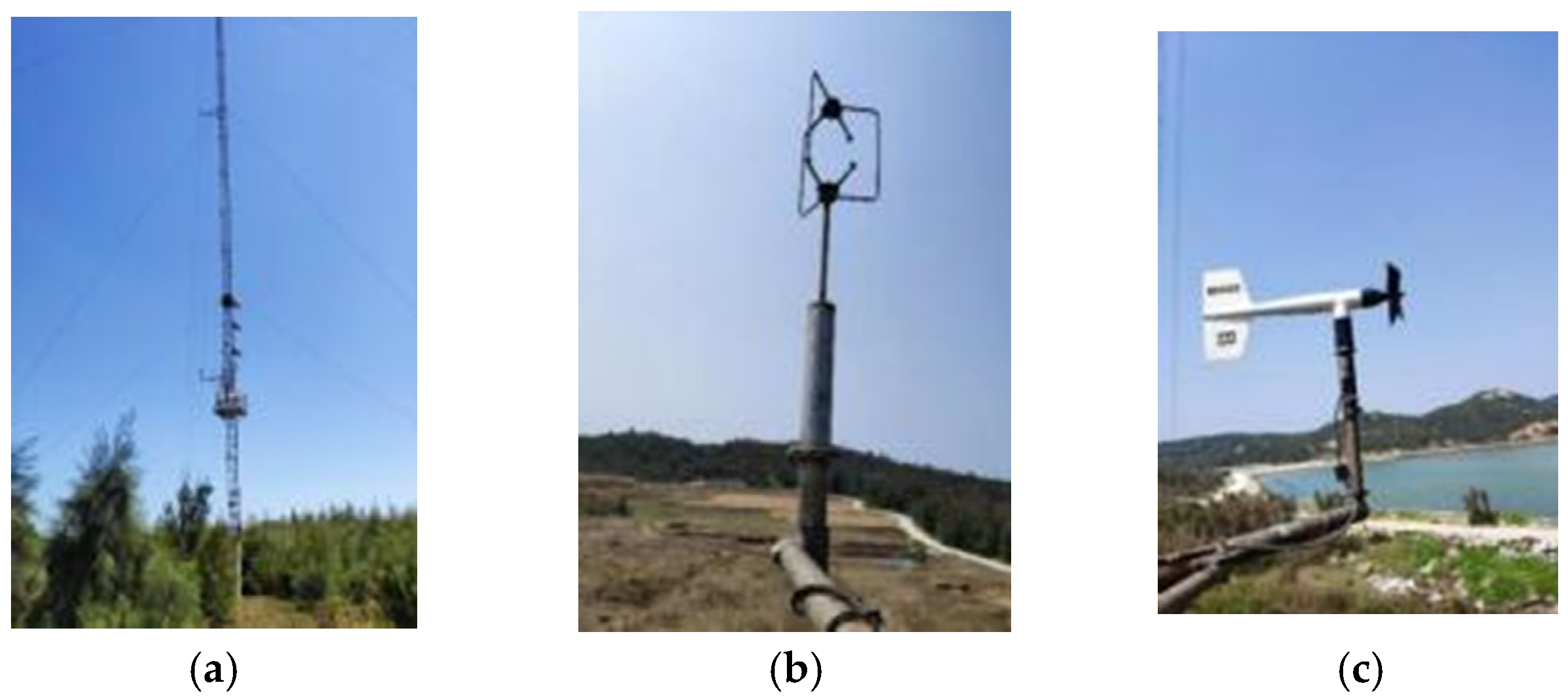
Natural wind data were obtained by the research team from a meteorological mast installed on Yutou Island, Pingtan County, Fujian Province. This coastal island region features open terrain with a surface roughness coefficient of 0.19, intermediate between Class B and Class C terrains. Wind field monitoring was conducted using a 3D sonic anemometer and a cup anemometer, as illustrated in Figure 1. For analysis, measured winter wind data from 24 January 2018 were selected. Wind monitoring was performed at multiple heights: 10 m, 30 m, 50 m, 80 m, 90 m, and 100 m above ground level. Figure 2 presents the recorded time histories of wind speed and turbulence intensity during the monitoring period.

Figure 1.
Wind field measurement instruments. (a) Wind tower, (b) Ultrasonic anemometer, (c) Vane wind meter.

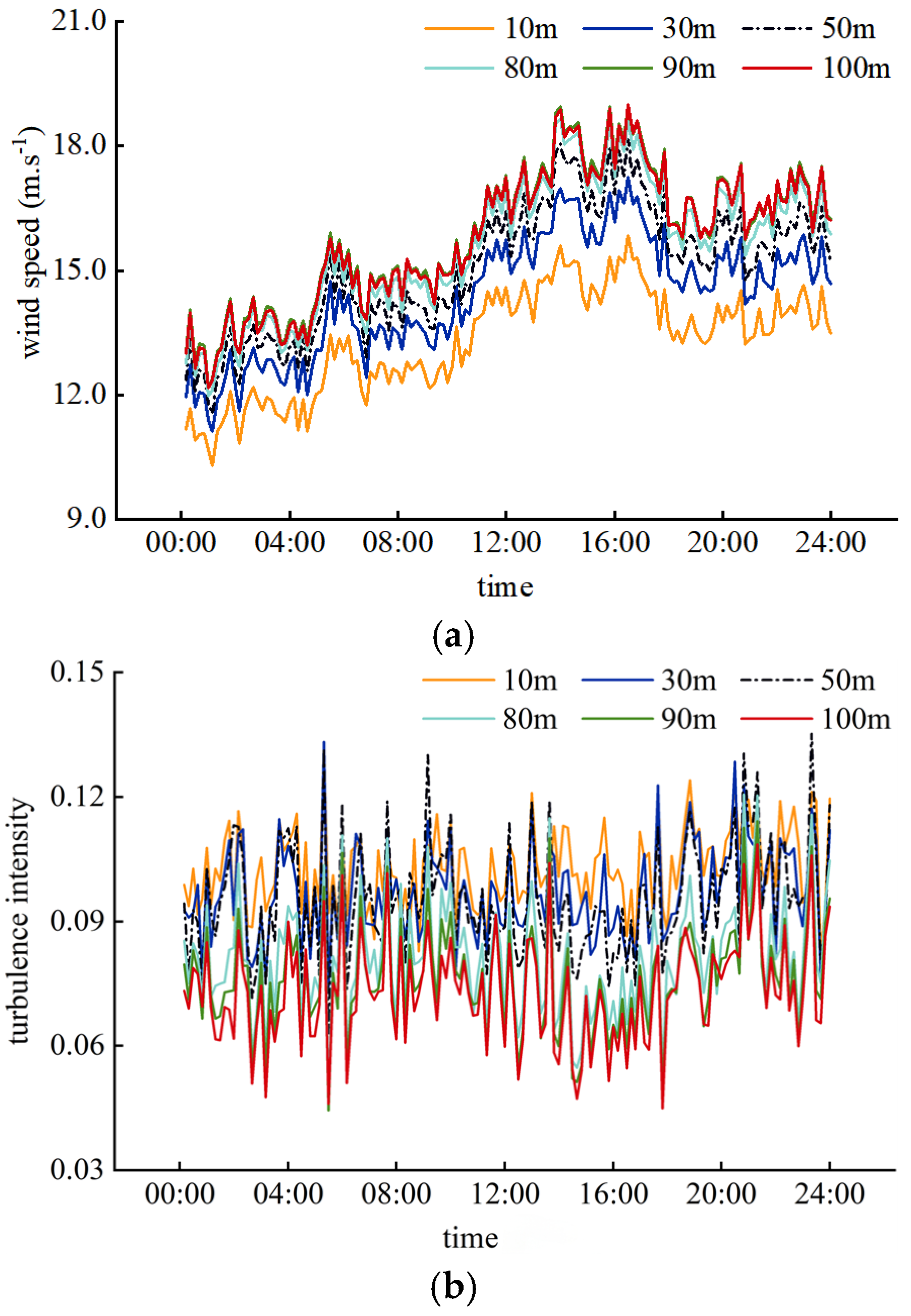
Figure 2.
Measured average wind characteristics. (a) Average wind speed at different heights, (b) Turbulence at different heights.
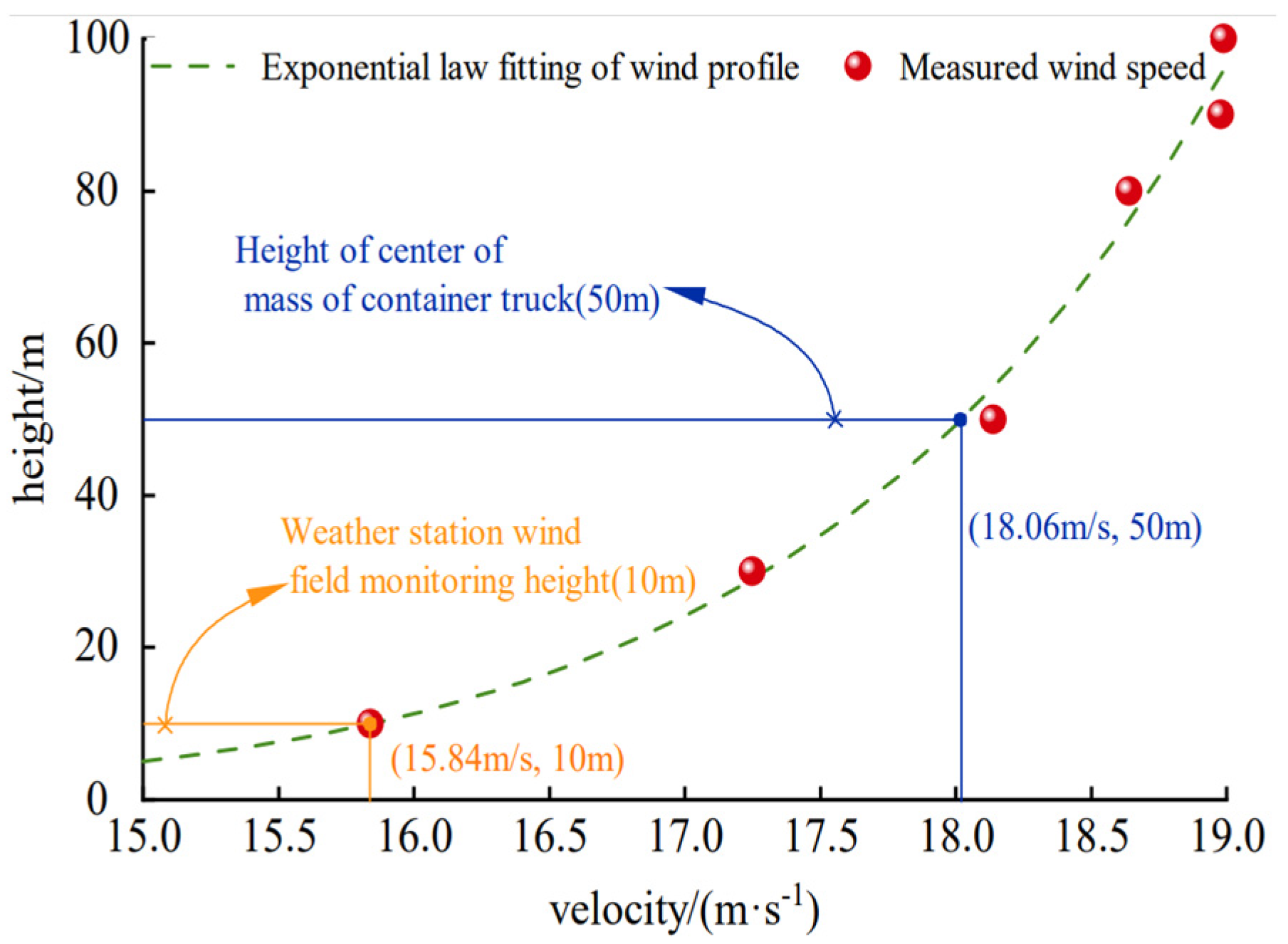
As shown in Figure 2, the wind speed exhibits significant variation between 10 m and 80 m due to topographic and geographical influences. With increasing elevation, the effect of surface roughness elements gradually diminishes, resulting in reduced wind energy dissipation. Consequently, the mean wind speed increases with height, while flow pulsation characteristics weaken, leading to progressively lower turbulence intensity. Surface roughness elements demonstrate negligible influence on wind speed at an elevation above 80 m. The wind energy dissipation remains consistent across different heights, causing minimal variation in the mean wind speed with further elevation increases and stabilized turbulence intensity. The highest mean wind speed occurred at 16:00 (local time). The wind speed profile at this time was fitted using the power law, as presented in Figure 3.

Figure 3.
Wind speed profiles.
The average wind speed is determined using Equation (1), the turbulence degree is determined using Equation (2), and the wind profile is determined using Equation (3).
where V is the wind speed (m/s); U is the 10 min average wind speed (m/s); σi is the root mean square value of the pulsating wind speed in the u (longitudinal), v (horizontal), and w (vertical) directions (m/s); (t2 − t1) represents different time intervals, with a 10 min average wind speed being used in this paper; α is the roughness index, with a fitted value of 0.08; z is the height (m); and zs is the standard height, which is set as 10 m.
3. Computational Model
3.1. Geometric Model
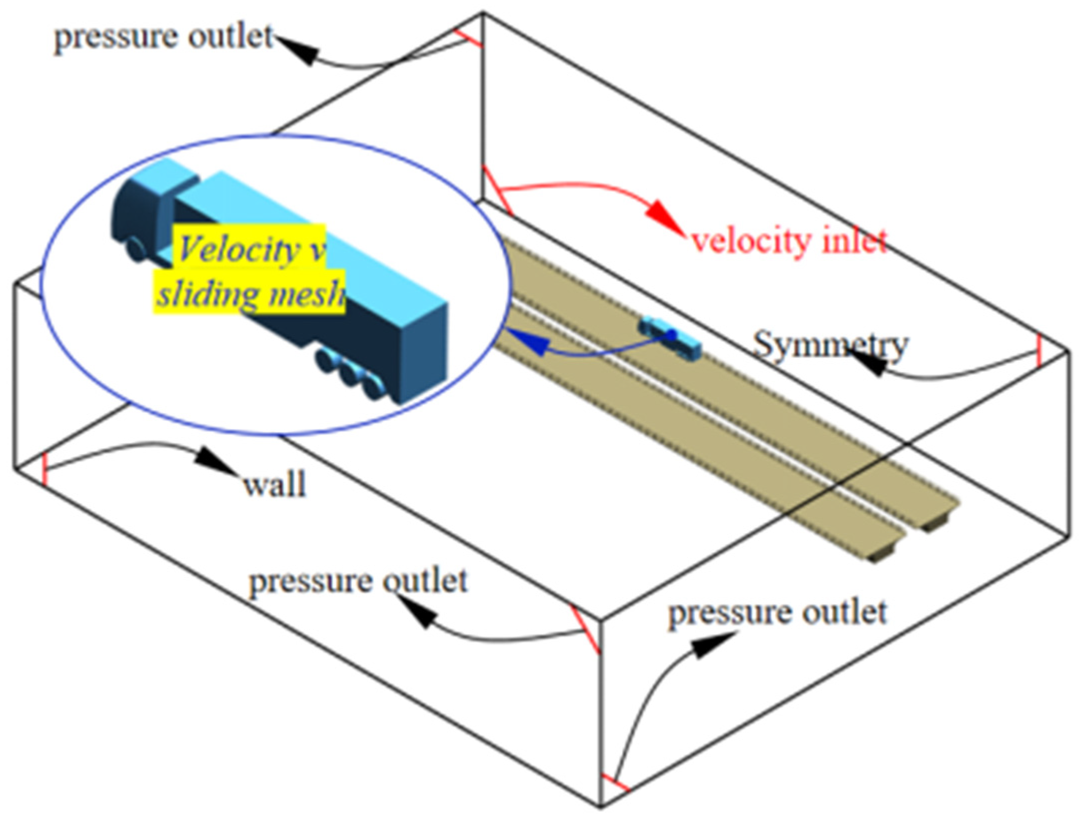
In this study, a bridge model in Fujian Province in China is taken as an example. Based on a prior analysis of wind conditions on the dual-girder bridge deck, the maximum inflow wind speed occurs at the highest clearance point of the bridge’s main span. Accordingly, this study adopts the cross-section at this location to establish a geometric model of a container truck traveling on the bridge, retaining the primary geometric features of both the truck and the dual-girder bridge, with a bridge cross slope of 1.5%. Considering the characteristics of bridge deck wind fields, the most critical operational scenario occurs when the container truck is positioned in the windward-side lane [17]. In accordance with the T/CSAE 112-2019 Technical Specification [18] for Aerodynamic Simulation of Passenger Vehicles, the geometric model for bridge-crossing vehicle analysis is constructed as illustrated in Figure 4.

Figure 4.
A geometric model of traffic on the bridge.
3.2. Discrete Phase Model (DPM)
The wind–rain environment essentially constitutes a gas–liquid two-phase flow. The raindrop is assumed to be an ideal sphere; therefore, the default standard spherical drag model (Spherical Drag Law) is applied for simulation. In this model, raindrops are simplified as regular spherical particles, with key rainfall parameters including the raindrop diameter, raindrop size distribution, terminal velocity, and mass flow rate. The relationship between the proportion of different-sized raindrops and rainfall intensity follows Equation (4), established by BEST [19] based on observational data. The raindrop size distribution is described using a Gamma distribution empirical formula [20], as presented in Equation (5).
where F is the percentage of the volume of raindrop particles with a diameter of less than or equal to r; r is the equivalent diameter of raindrops, which ranges from 0.1 mm to 6 mm; I represents the rainfall intensity, with five conditions set in the text, namely, 50 mm/h, 100 mm/h, 150 mm/h, 200 mm/h, and 250 mm/h; W is the total volume of raindrops per unit volume of air (mm3/m3); N(r) is the number of raindrops per unit volume (m−3·mm−1); N0 is the concentration parameter (m−3·mm−1); Λ is the size parameter (mm−1); and μ indicates the spectrum type, with a value of 2. Other constant parameters are set as follows: B1 = 1.3, B2 = 67, p = 0.232, q = 0.846, and n = 2.25.
Raindrops with different diameters have varying falling speeds [21,22], as determined using Equation (6). The terminal velocity of the raindrop is determined by the weighted average velocity in Equation (7). The mass flow rate of the discrete phase entering the calculation area within a unit time is determined using Equations (8) and (9). The distribution relationship between particle number and particle diameter is determined using Equation (10).
where V(r) is the final velocity (m/s) of the raindrop; M1 is the mass entering the computational domain per unit time and area (kg/s m2); M2 is the total mass entering the computational domain per unit time (kg/s); S is the incident area of the discrete phase particles (m2); is the median diameter (mm); Yr is the mass fraction of raindrops larger than this diameter; and n is the distribution index. The initial condition parameters for the discrete phase under different rainfall intensities are shown in Table 1.

Table 1.
Settings of discrete phase model parameters.
3.3. Computational Methodology
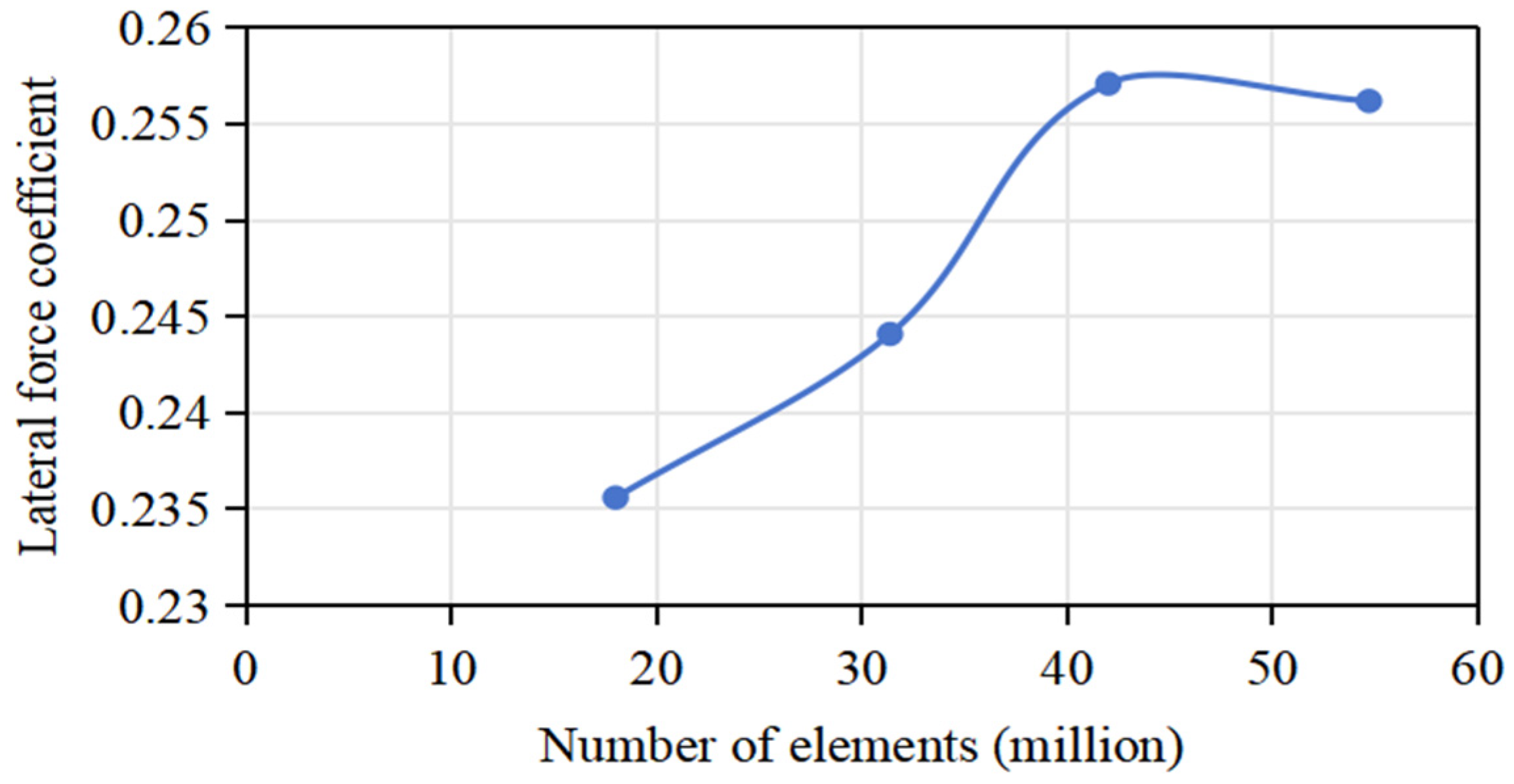
A coupled aerodynamics–system dynamics approach was employed to investigate the crosswind stability of vehicles on bridges. The computational domain was discretized using a hybrid mesh scheme featuring polyhedral cells near the rainfall surface and wall boundaries and hexahedral cells in the core region. The volume mesh surrounding the truck was progressively refined, with a core resolution of 80 mm. The surface mesh size was set to 32 mm, accompanied by four boundary layers with a growth ratio of 1.1, and the height of the first layer was 1 mm. The final mesh comprised approximately 42 million cells after grid independence verification under different meshing styles in Table 2 and Figure 5. The computational model was validated against wind tunnel tests [23], demonstrating satisfactory accuracy, as illustrated in Figure 6. The conditions in the simulation were set the same as in the reference [23]. In the wind tunnel experiment [23], the aerodynamic drag coefficient of the vehicle was 0.259, and the verification data of this simulation is 0.257. The error between the numerical simulation value and the wind tunnel experiment value is around 5%, indicating that the slip grid method can effectively simulate the driving of the vehicles.
Table 2.
Lateral force coefficient under different meshing strategies.

Figure 5.
Lateral force coefficients under different meshing strategies.

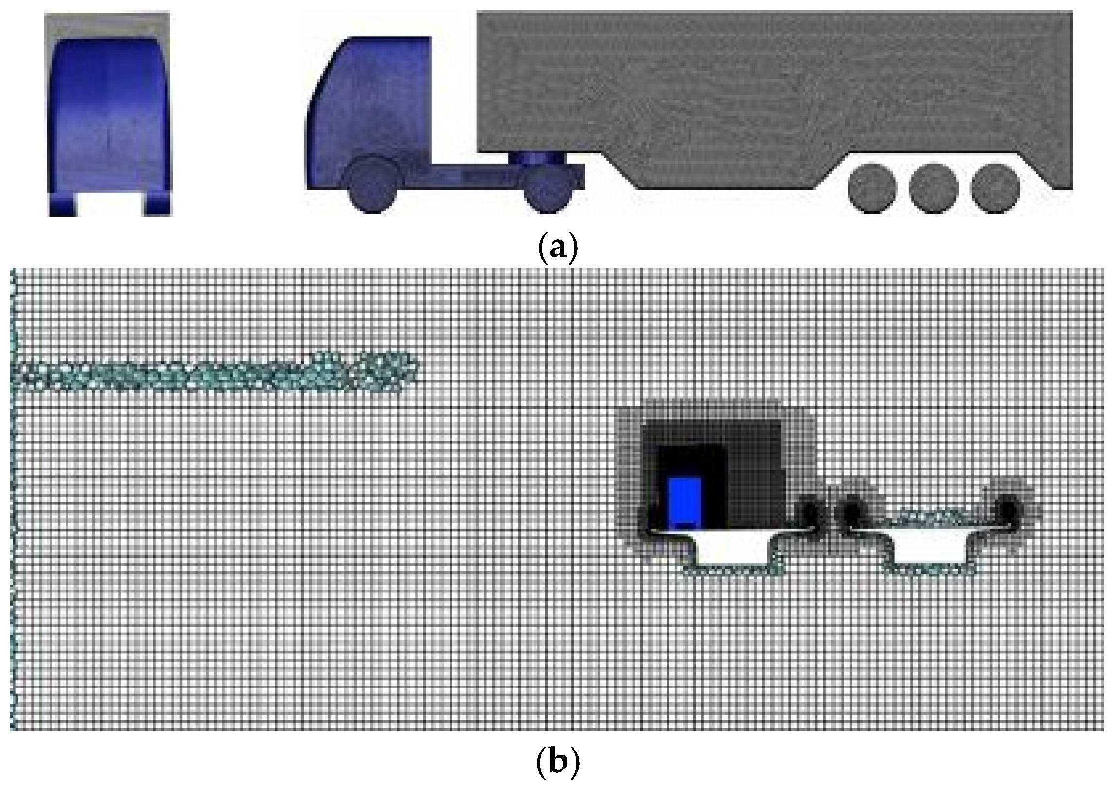
Figure 6.
Meshing of calculation domain. (a) Surface grid, (b) Body grid.
For the aerodynamic analysis of bridge-crossing vehicles, a sliding mesh technique was implemented, with the container truck traveling at 80 km/h. The sliding mesh model includes a stationary region and a moving region, which are dynamically coupled through an interface. During the transient solution process, flow data are transmitted through this interface, ensuring flux conservation. By considering rigid motion as vehicle displacement, the model accurately captures non-steady flow effects through transient calculations, making it suitable for numerical simulations of moving boundaries, such as vehicle outflow fields. The time step size is 0.0005 s, the simulation time is 1.5–2 s, the number of processors used is 90 threads, and the calculation time of one condition is 7–10 days. The realizable k-ε turbulence model and second-order upwind scheme were adopted for numerical solution. Three inflow boundary conditions were considered: (1) uniform flow, (2) wind profile with low turbulence intensity (TI), and (3) wind profile with high TI. The wind profiles were prescribed via UDF using the power-law fitting curve in Figure 3. Based on the measured wind speed data, the mean turbulence intensity(7.76%) was calculated and set as input values in the simulations. To show the influence of turbulence intensity, the low value of 0.5% was applied for comparison. The high-TI condition (7.76%) corresponded to the turbulence intensity at the truck’s centroid height, while the low-TI condition was set to 0.5%. The uniform flow velocity was specified as 18.06 m/s at the truck’s centroid height.
The coupled simulation employed a Eulerian–Lagrangian approach through the DPM, treating wind as the continuous phase and raindrops as the discrete phase with gravitational effects. The key parameters for the simulation are summarized in Table 2.
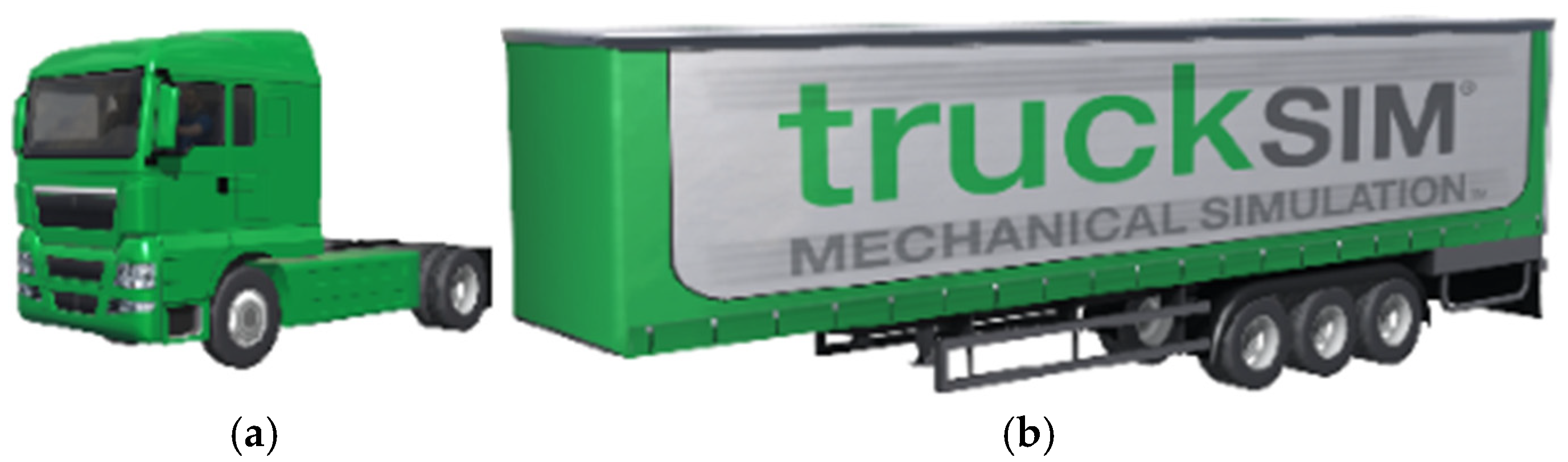
Finally, a multi-body dynamic model of a container truck driving on the bridge under non-load conditions was established according to the bridge route. The influence of route curvature and crosswind was comprehensively considered. The main parameters of the tractor and semi-trailer are shown in Table 3, and the truck model is shown in Figure 7.
Table 3.
Main parameters of container trucks.

Figure 7.
Truck dynamic model. (a) Tractor, (b) Semi-trailer.
Based on the aerodynamic analysis results obtained under coupled wind–rain conditions, the corresponding aerodynamic forces and moments were applied at the centroid positions of both the tractor and semi-trailer for each operational scenario. These loads were implemented as a gust excitation with a 3 s duration. Directional control was achieved through a preview-follower driver model with a preview time of 1.4 s.
For rainfall conditions, the relationship between precipitation intensity and water film thickness was determined using Equation (11). The road adhesion coefficient was characterized as a function of both post-rainfall water film thickness and vehicle speed. The adhesion coefficient under partial hydroplaning conditions was calculated using Equation (12) [24,25].
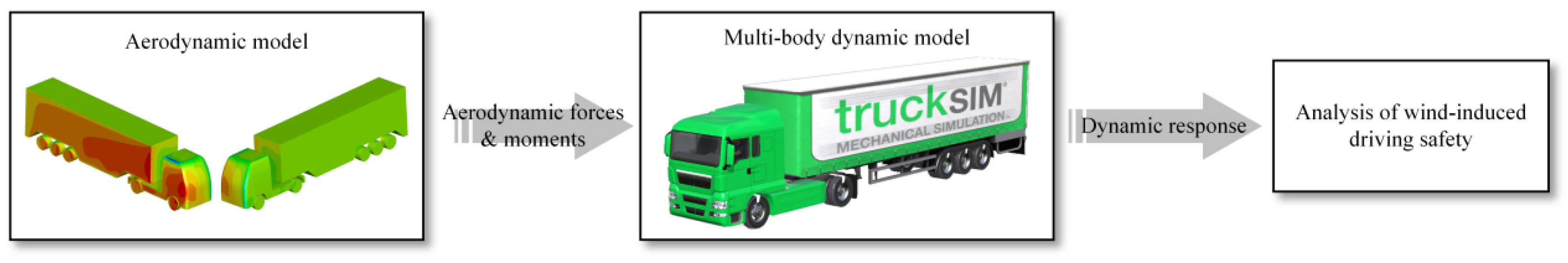
where h is the water film thickness (mm); φ is the road adhesion coefficient; v is the speed of the container truck, set to 80 km/h; l is the slope length (m); i is the bridge gradient, set to 1.5%; I is the rainfall intensity (mm/min); and TD is the construction depth (mm). The corresponding bridge surface adhesion coefficients for rainfall amounts of 0, 50, 100, 150, 200, and 250 mm/h are 0.70, 0.58, 0.49, 0.40, 0.33, and 0.26, respectively. The software ANSYS 2021 was used for the pneumatic part, and TruckSim 2019 was applied for the system dynamics part. In the simulation, the static coupling simulation method was applied for simulation using the Truck Sim software platform. The route curvature of the considered cross-sea bridge is very small; therefore, it is simplified as a straight line, and the bending of the bridge is neglected. The aerodynamic load under different working conditions is calculated by the computational fluid dynamics (CFD) method, and it is applied to the vehicle dynamic model as the external disturbance quantity, and the transient response of the vehicle dynamics under different working conditions can be obtained. The simulating procedure can be seen in Figure 8. Specifically, the interactions between the vehicle and crosswinds were simulated by the aerodynamic module. The crosswinds were modeled using a stepwise gust model, and the driver’s pre-aim model was used to simulate the actual driving behavior of the driver, which can help obtain the dynamic response of the vehicle under crosswind, thereby evaluating the overall stability of the vehicle under crosswind. Moreover, it should be mentioned that, according to T/CSAE 112-2019, the aerodynamic drag coefficient is a curve that changes with each time step. The number of internal iterations should be adjusted based on the convergence within a single time step, ensuring that the physical duration is at least two vehicle lengths. And the aerodynamic drag coefficient should periodically fluctuate within 0.5 s before the stop. Therefore, the CFD results in this simulation are the average values calculated over the 0.5 s before the stop of vehicles.

Figure 8.
Simulating procedure of vehicle dynamics.
4. Results and Discussion
4.1. Influence of Wind Field
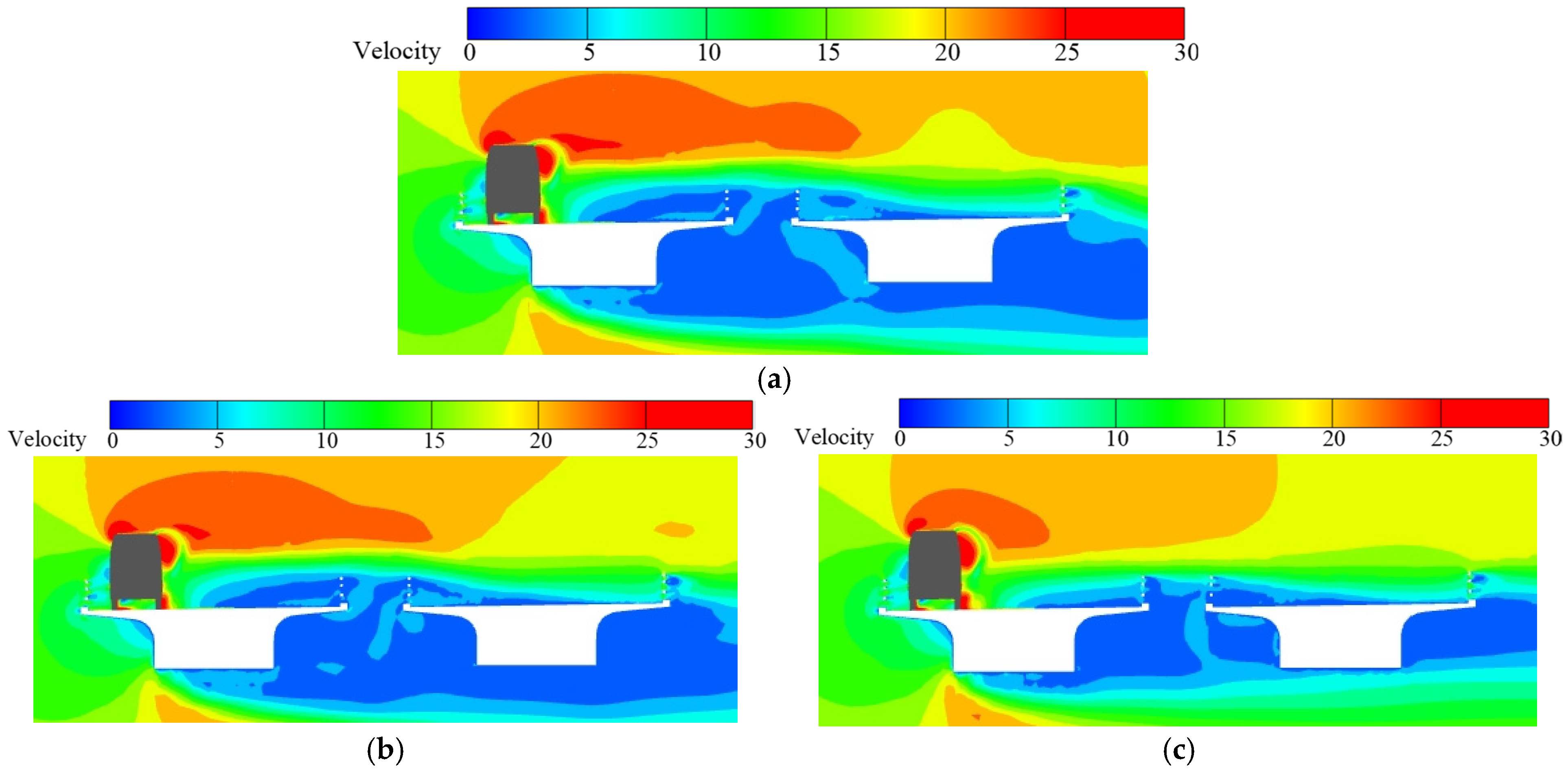
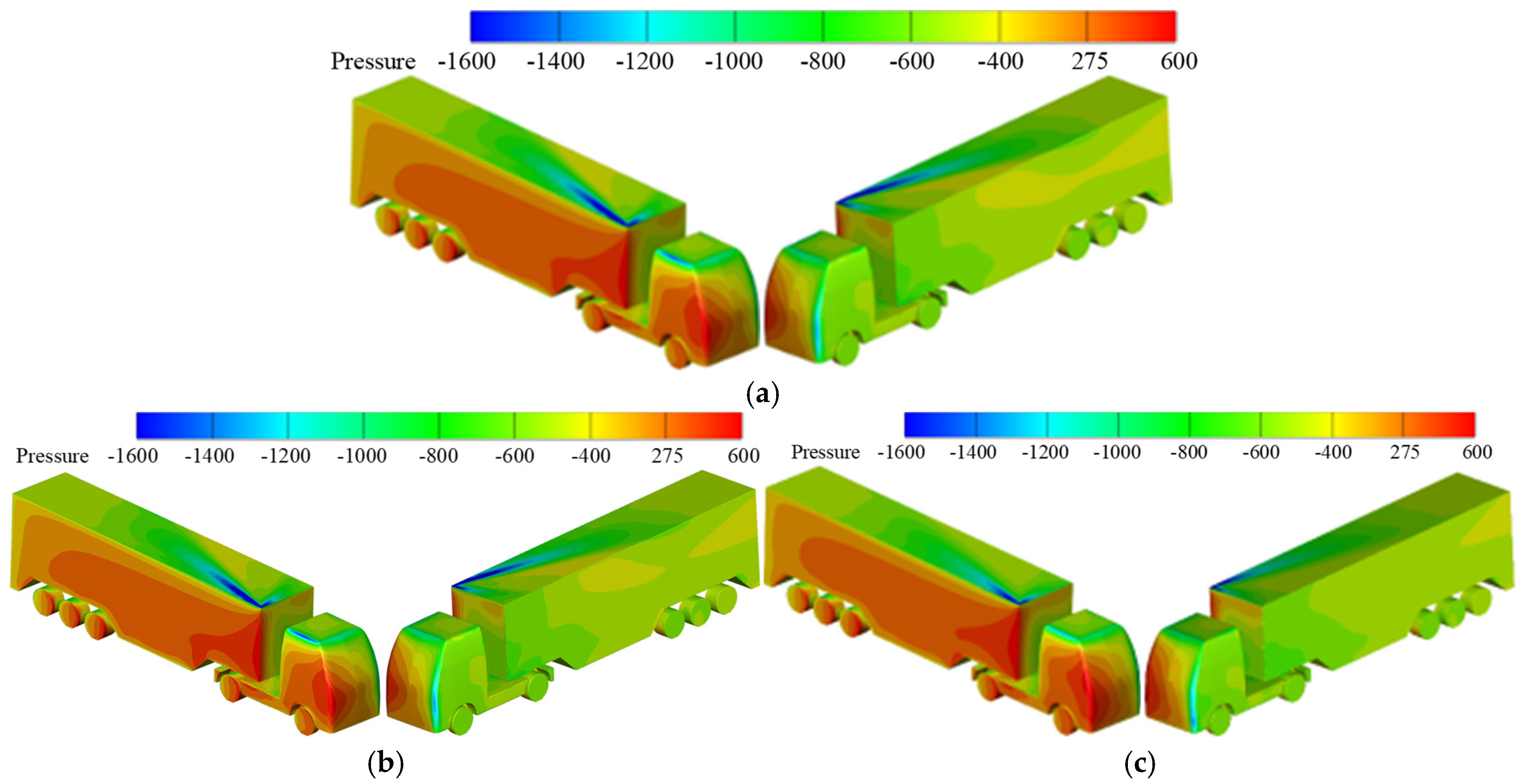
Figure 9 illustrates the influence of different crosswind loading patterns on the flow field around the tractor’s front axle section under a rainfall intensity of 100 mm/h. With identical turbulence intensity levels, the simulation results demonstrate that uniform inflow (based on the wind speed at the vehicle’s centroid height) and wind profile inflow produce negligible differences in the truck’s surrounding flow field characteristics. However, when incorporating the actual turbulence intensity measured at the truck’s centroid height into the wind profile inflow condition, significant flow field modifications can be seen. Enhanced wind pulsatility and increased velocity fluctuations lead to elevated wind speeds across the bridge deck. As shown in Figure 10, both the windward-side positive pressure zone and leeward-side negative pressure zone surrounding the semi-trailer are amplified, with measurable increases in pressure magnitude.

Figure 9.
Wind speed distribution around truck under different wind fields. (a) Uniform flow, (b) Wind profile with low turbulence intensity, (c) Wind profile with high turbulence intensity.

Figure 10.
Wind pressure distribution around truck under different wind fields. (a) Uniform flow, (b) Wind profile with low turbulence intensity, (c) Wind profile with high turbulence intensity.
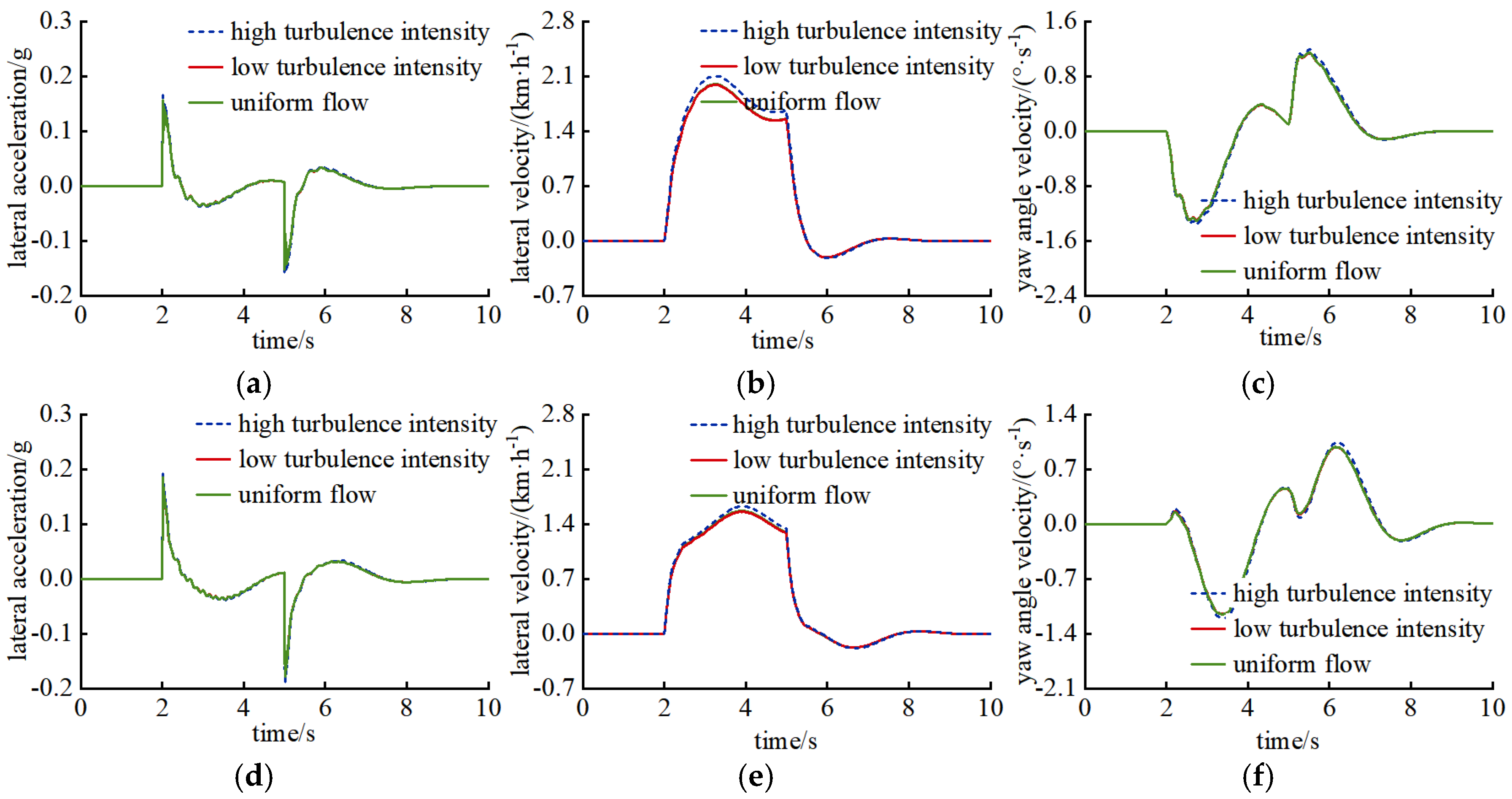
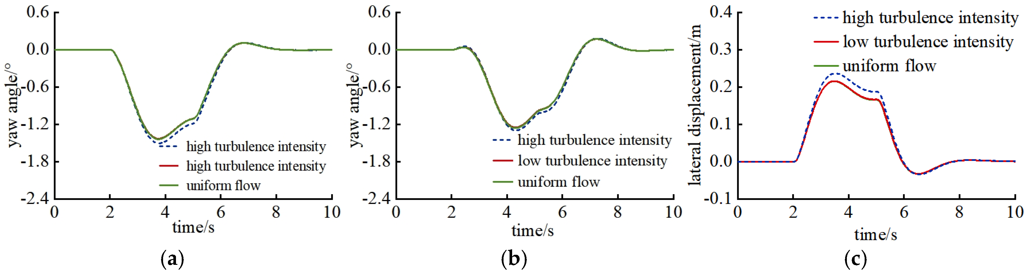
As shown in Table 4, the aerodynamic effect of uniform flow and wind profile flow on freight vehicles is negligible. However, based on wind profile flow, considering the actual turbulence intensity, the lateral force coefficients of both the tractor and the semi-trailer increased by 8.4% and 5.1%, respectively; the lift coefficient of the tractor slightly increased; and the drag coefficient markedly increased by 26.7%. The drag and lift coefficients of the semi-trailer decreased by 6.1% and 13.6%, respectively. Figure 11 and Figure 12 illustrate the impact of different crosswind loading forms on the lateral sway and yaw motion responses of the tractor and semi-trailer, consistent with previous aerodynamic analysis results. Under the same turbulence intensity, the effect of uniform flow and wind profile flow on the motion of freight vehicles is relatively small. After considering the actual turbulence intensity, the increases in the peak lateral acceleration, lateral speed, and yaw rate of the tractor are 6.4%, 4.5%, and 4.3%, respectively, while the increases for the semi-trailer are 6.0%, 4.5%, and 5.2%. The increases in the peak yaw angle for the tractor and semi-trailer are 5.2% and 3.8%, respectively, and the increase in the displacement of the vehicle’s center of gravity is 9.8%. In summary, using the wind speed at the height of the freight vehicle’s center of gravity is equivalent to the effect of uniform flow and wind profile flow, and the lateral stability of the freight vehicle is mainly related to the wind field at the height of the bridge surface.
Table 4.
Influence of wind field on aerodynamic coefficient.

Figure 11.
Response of side bias and lateral movement of container trucks under different wind fields. (a) Lateral acceleration of tractor, (b) Lateral velocity of tractor, (c) Yaw velocity of tractor, (d) Lateral acceleration of semi-trailer, (e) Lateral velocity of semi-trailer, (f) Yaw velocity of semi-trailer.

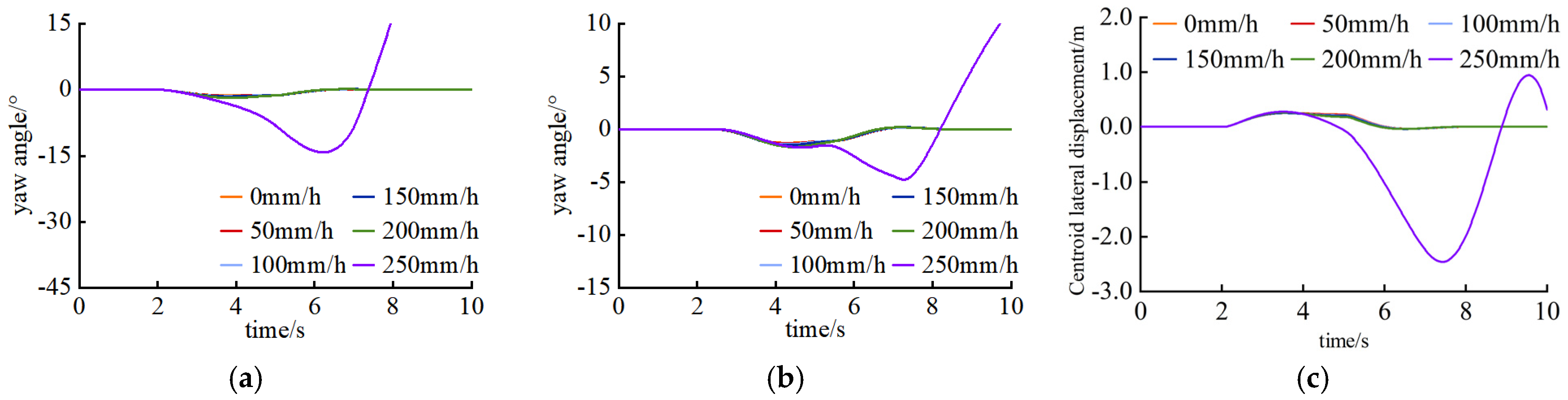
Figure 12.
Lateral swing angle and lateral displacement of container trucks under different wind fields. (a) Yaw angle of tractor, (b) Yaw angle of semi-trailer, (c) Lateral displacement of centroid.
4.2. Influence of Rainfall
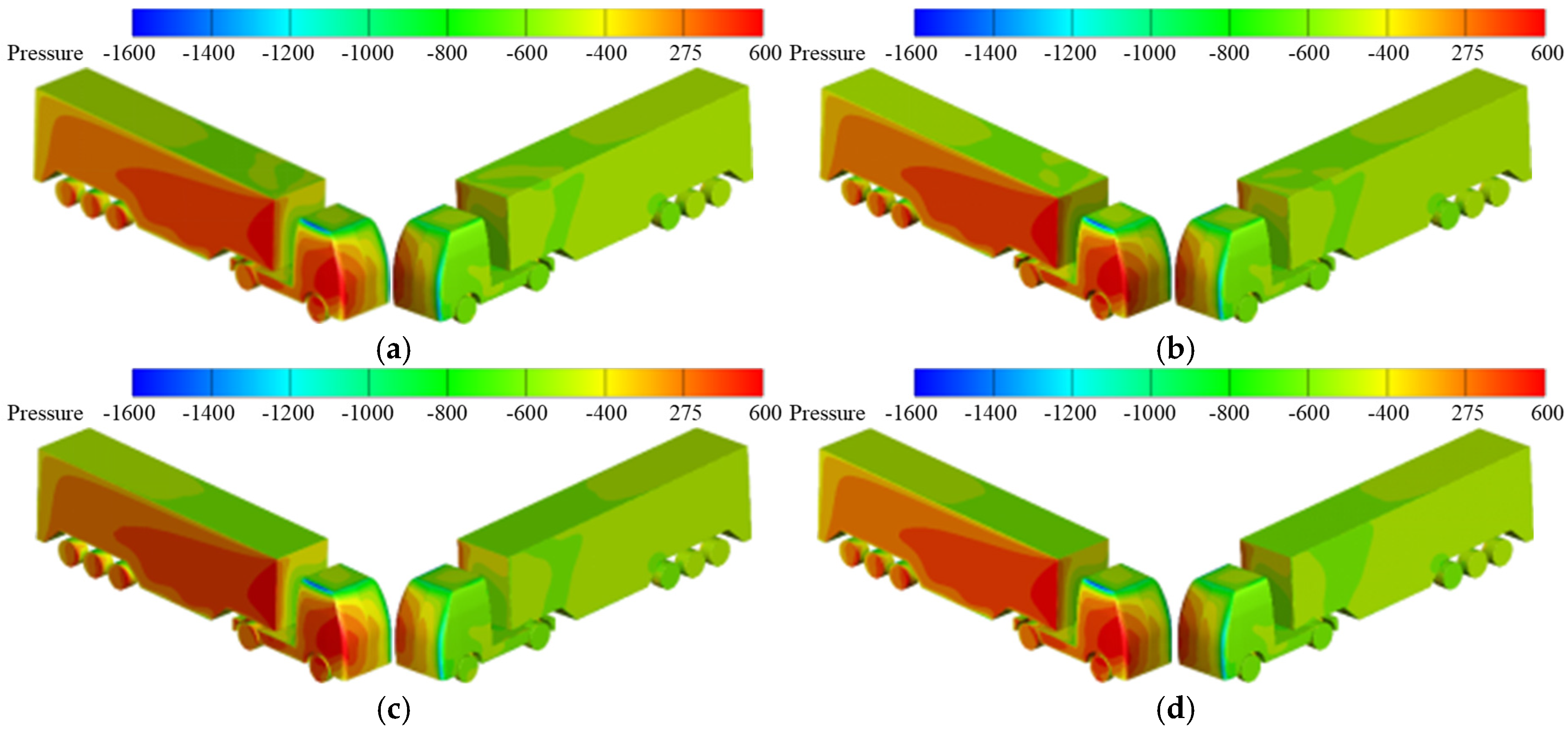
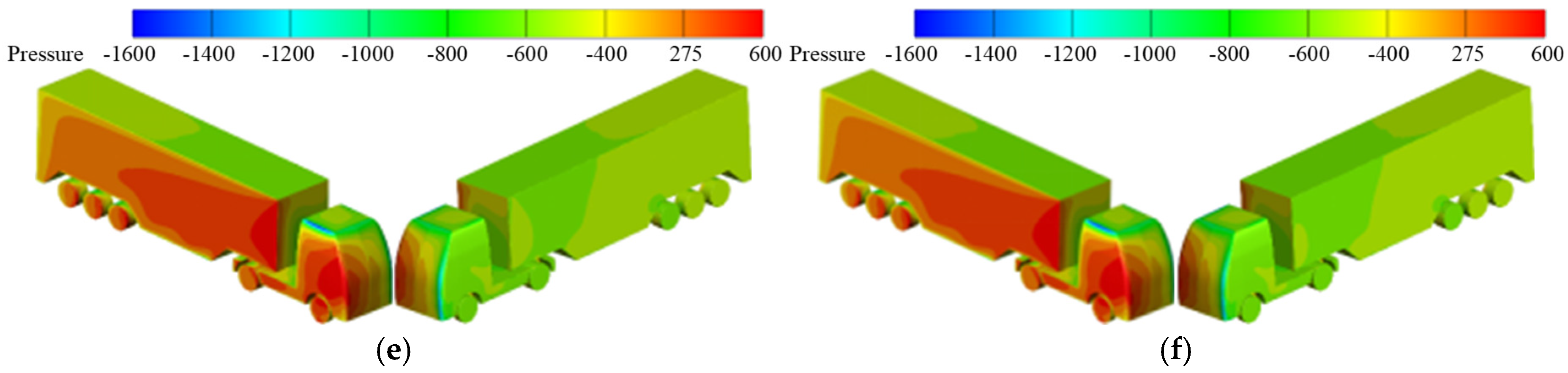
Figure 13 shows the effect of different rainfall conditions on the surface pressure distribution of container trucks when the wind speed at the height of the truck’s center of mass is 20.8 m/s. The wind speed on the windward side of the container truck is higher, where the gas phase plays a dominant part, and the rain phase has less influence. The similar flow field indicates that the increase in rainfall has little impact on the flow field on the windward side of the truck. The positive pressure area of the truck hardly changes. However, at the top of the truck and on the leeward side, the wind speed is lower, the energy transfer between the rain phase and the gas phase is stronger, and the airflow velocity in the local area increases, resulting in a significant increase in the negative pressure area at the front end of the top of the tractor and the front end of the leeward side.
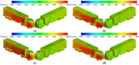

Figure 13.
Surface pressure distribution of truck with different rainfalls. (a) 0 mm/h, (b) 50 mm/h, (c) 100 mm/h, (d) 150 mm/h, (e) 200 mm/h, (f) 250 mm/h.
Table 5 compares the influence of rainfall with or without rain phase on the aerodynamic force of trucks when there is 250 mm/h of rainfall. After considering the influence of the rain phase, the aerodynamic resistance of the tractor increases significantly, and the aerodynamic resistance of the semi-trailer decreases because the water film formed by the rain is conducive to reducing the frictional resistance. Rain has a great influence on the aerodynamic lift and aerodynamic lateral force of the semi-trailer, where the aerodynamic lift coefficient increases by 17.7%.
Table 5.
Influence of rainfall on aerodynamic coefficient.
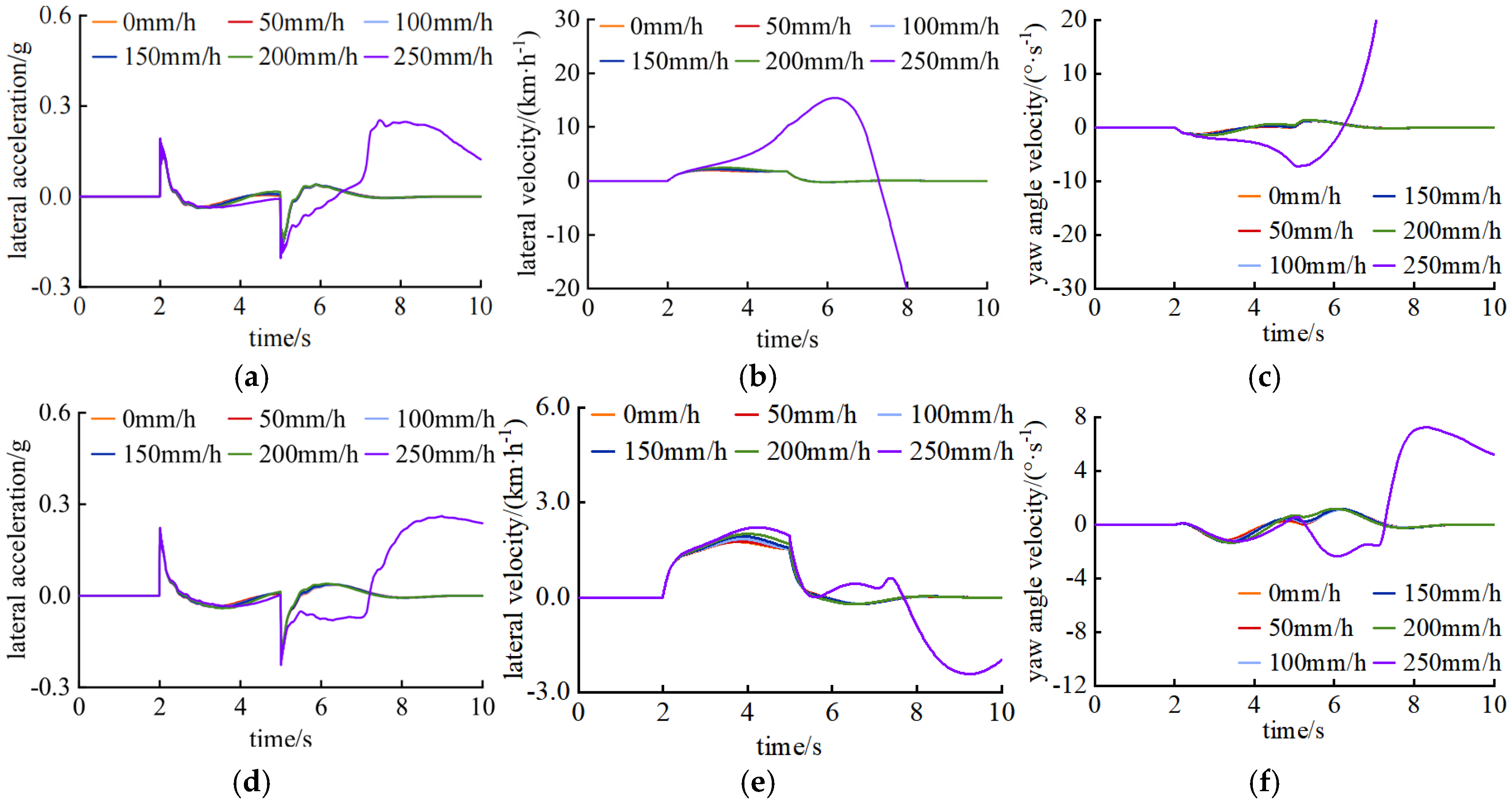
Figure 14 and Figure 15 show the influence of different rainfall conditions on the dynamic responses of trucks. The peak lateral acceleration of tractors at the moment of wind and rain coupling reaches 0.19 g, and that of semi-trailers is 0.22 g. When the rainfall increases from 0 to 200 mm/h, the lateral speed of the tractor increases from 1.97 km/h to 2.49 km/h, and the lateral speed of the semi-trailer increases from 1.75 km/h to 2.01 km/h. The yaw angle velocity of the tractor increases from 1.25°/s to 1.49°/s, and the yaw angle velocity of the semi-trailer increases from 1.17°/s to 1.34°/s. The yaw angle of the tractor increases from 1.33° to 1.86°, the yaw angle of the semi-trailer increases from 1.28° to 1.67°, and the lateral displacement of the center of mass of the truck increases from 0.25 m to 0.27 m.

Figure 14.
Response of container trucks to lateral drift and yaw motion under different rainfall amounts. (a) Lateral acceleration of tractor, (b) Lateral velocity of tractor, (c) Yaw angle velocity of tractor, (d) Lateral acceleration of semi-trailer, (e) Lateral velocity of semi-trailer, (f) Yaw angle velocity of semi-trailer.

Figure 15.
Skew angle and lateral displacement of container trucks under different rainfall conditions. (a) Yaw angle of tractor, (b) Yaw angle of semi-trailer, (c) Centroid lateral displacement.
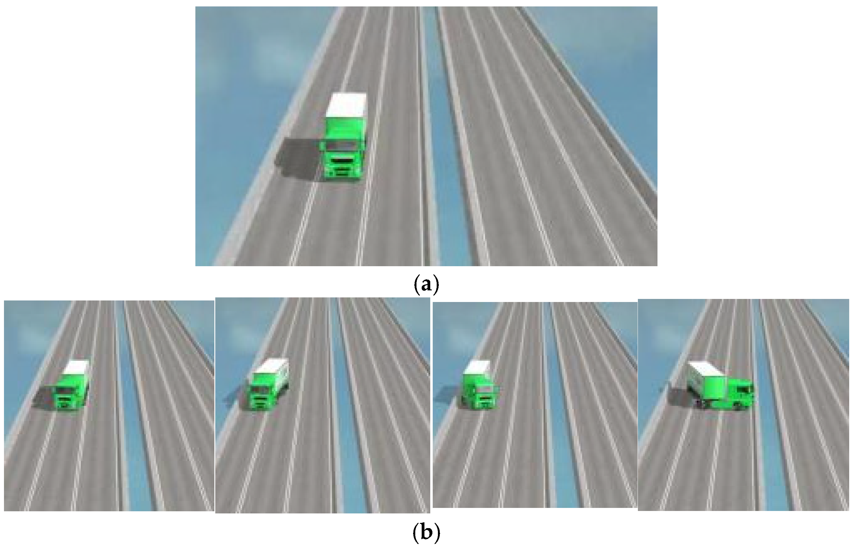
With the gradual increase in rainfall, although the lateral deviation movement and the yaw motion of the truck are more obvious, the driver feedback can still control the overall movement of the truck. When the rainfall increases to 250 mm/h, the road surface adhesion capacity is further reduced. The semi-trailer appears to be sideways after the crosswind effect and drives into the adjacent lane, and sideslip occurs after the vehicle is towed. After the crosswind disappears, the lateral speed and the yaw angle velocity of the tractor are in a parabolic rising state, the tractor cannot return to the predetermined straight driving trajectory, and the truck loses control and rushes out of the bridge deck, as shown in Figure 16.

Figure 16.
Response of container truck to side sliding motion. (a) Normal conditions, (b) Sideslip instability process.
4.3. Influence of Wind Speed
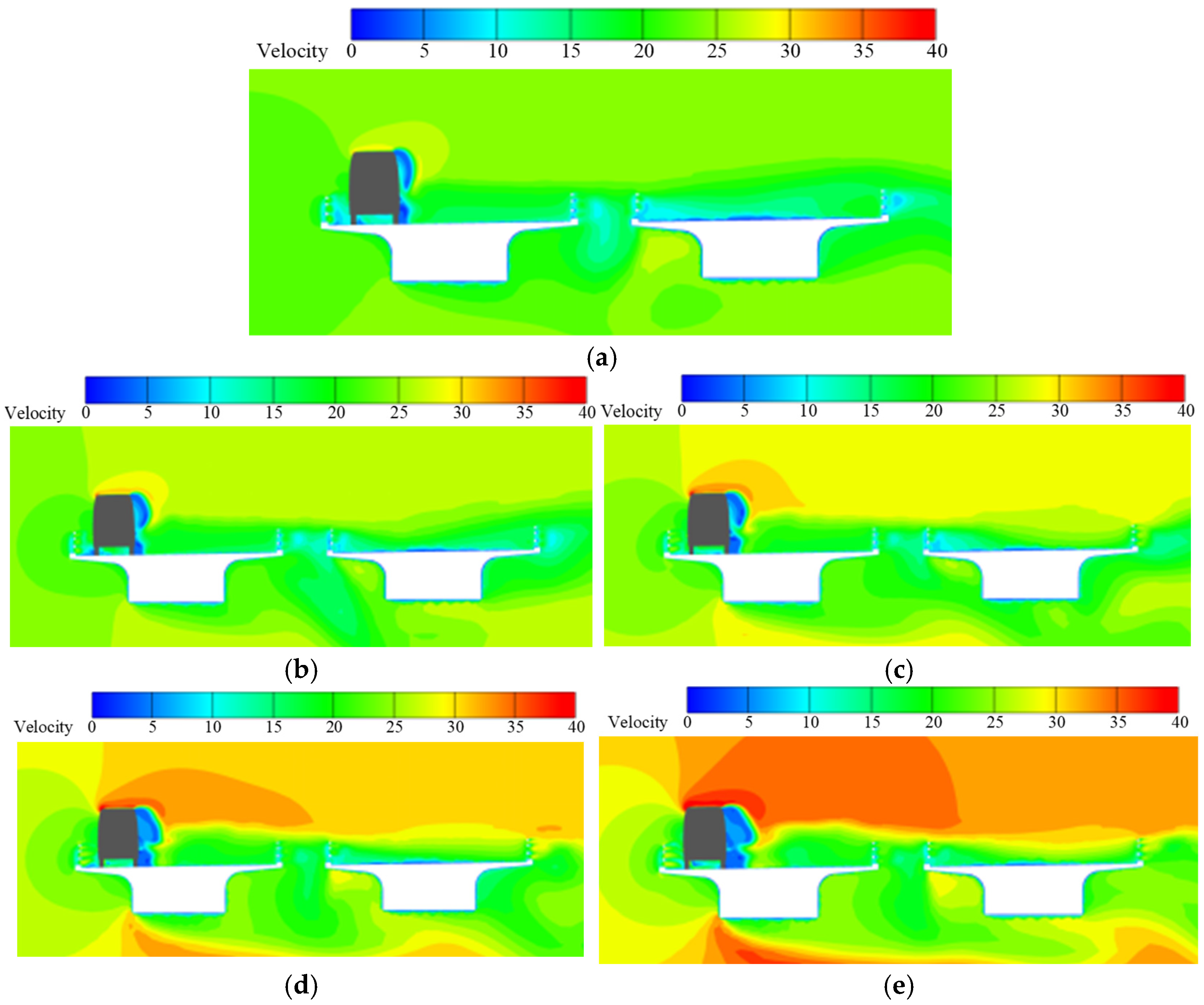
Figure 17 and Figure 18 show the influence of wind speed at the height of the centroid on the flow field and surface pressure distribution around the truck when the rainfall is constant (100 mm/h).

Figure 17.
Wind speed distribution around the truck with different side winds. (a) 10.8 m/s, (b) 13.9 m/s, (c) 17.2 m/s, (d) 20.8 m/s, (e) 24.5 m/s.

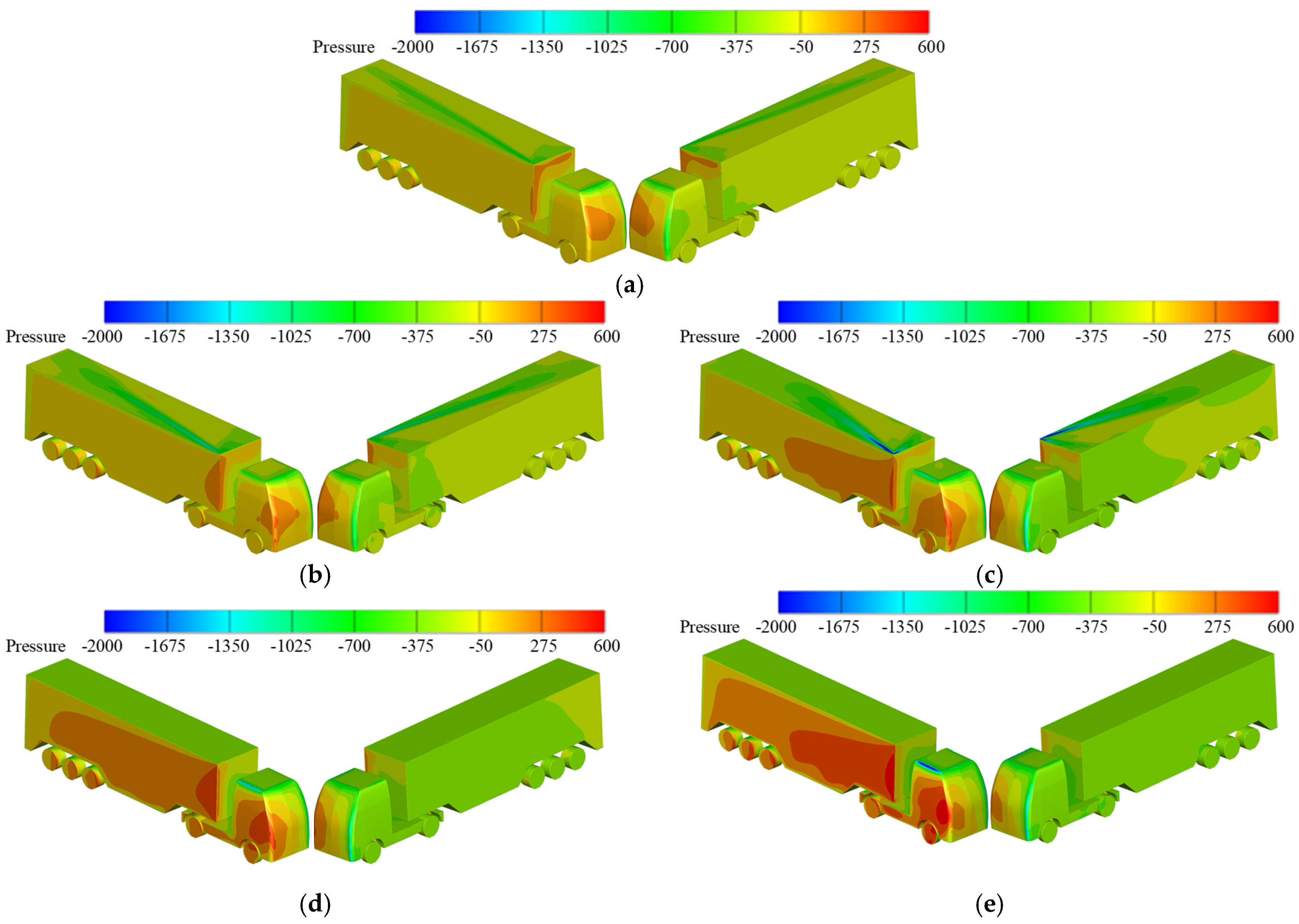
Figure 18.
Surface pressure distribution of truck with different side winds. (a) 10.8 m/s, (b) 13.9 m/s, (c) 17.2 m/s, (d) 20.8 m/s, (e) 24.5 m/s.
The wind speed on the windward side of the truck increases with the increase in crosswind speed, resulting in a gradual increase in the positive pressure area and positive pressure on the windward side of the tractor and semi-trailer. As the airflow separation zone on the leeward side gradually increases, the negative pressure area on the leeward side of the truck gradually spreads to the rear, and the negative pressure gradually decreases with the increase in wind speed. The increase in wind speed has a greater impact on the positive pressure on the windward side and the negative pressure on the leeward side than the increase in rainfall.
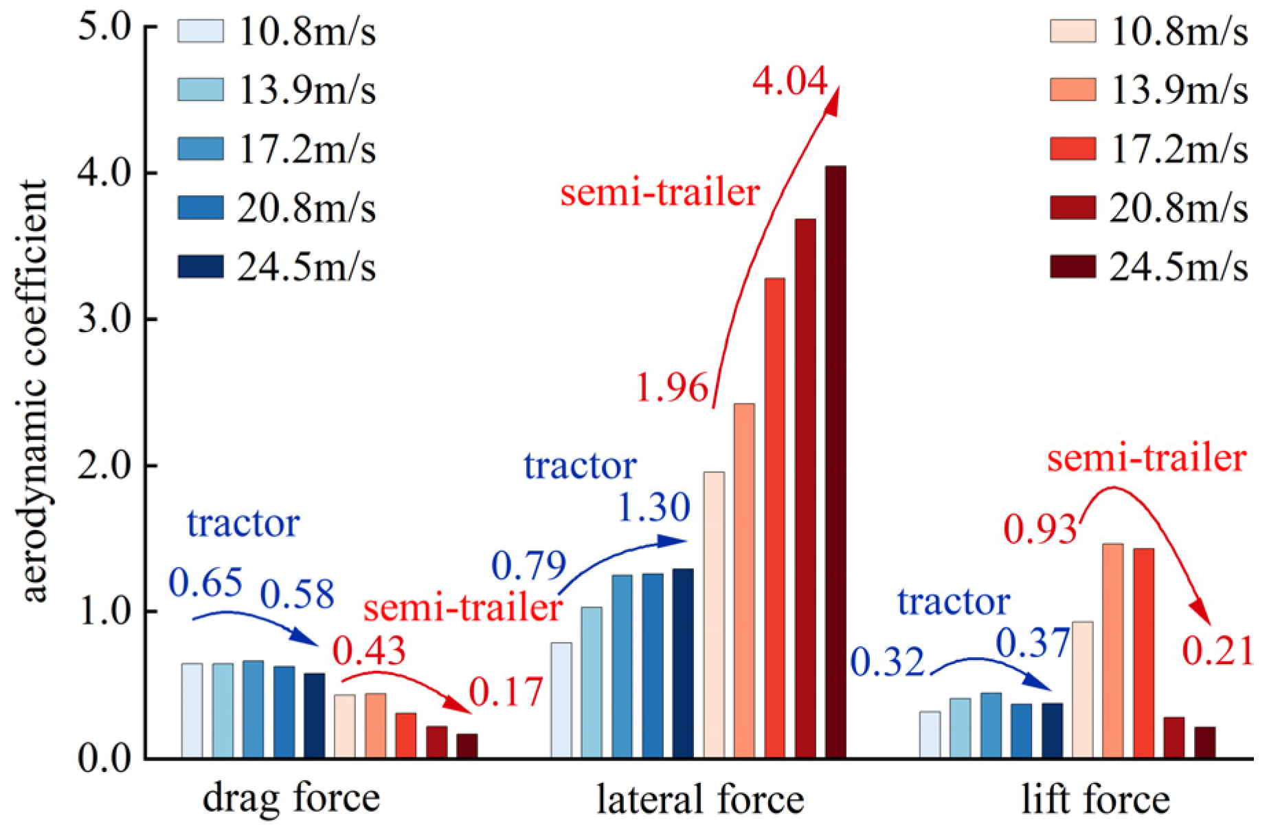
As indicated in Figure 19, the change in the pressure distribution of the truck body leads to a significant change in aerodynamic forces. The aerodynamic drag coefficient and aerodynamic lift coefficient of the tractor and semi-trailer first increase and then decrease with the increase in wind speed, while the aerodynamic lateral force coefficient increases with the increase in wind speed, indicating that the influence of wind speed on the aerodynamic lateral force of the semi-trailer is particularly obvious. When the wind speed increases from 10.8 m/s to 24.5 m/s, the aerodynamic side force of the tractor is 2.9 times that of the original value, and the aerodynamic side force of the semi-trailer is 3.7 times that of the original value. Therefore, compared with the variation in rainfall (Table 4), the change in wind speed has a more significant effect on the aerodynamic moment of container trucks, resulting in significant changes in the side wind stability of container trucks. Combining with Figure 18, it can be seen that with the increase in wind speed, the wind flow between the tractor and the trailer increases, resulting in the gradual decrease in air pressure on the front of the trailer; therefore, the aerodynamic resistance of the trailer gradually decreases with the increase in wind speed. When the wind speed increases from 10.8 m/s to 24.5 m/s, the positive pressure area on the windward side of the tractor and trailer gradually increases, while the negative pressure area on the leeward side also gradually increases with decreasing absolute values, which makes the aerodynamic lateral force increase sharply. When the wind speed is between 10.8 m/s and 20.8 m/s, the change in the trailer’s positive pressure zone mainly occurs in the front, resulting in the increase in the moment on the front side of the trailer’s center of mass, thus making the trailer’s yawing moment increase significantly. When the wind speed is 24.5 m/s, the lateral component of the composite wind speed increases, resulting in a significant increase in the aerodynamic pressure at the front and rear of the trailer, resulting in only a small increase in the yaw moment.

Figure 19.
Aerodynamic coefficients of trucks with different crosswind conditions.
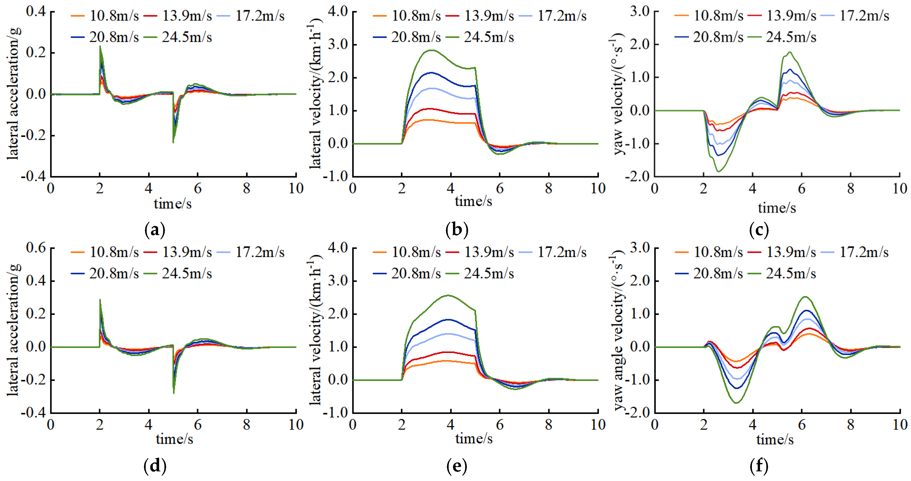
Figure 20 shows that the lateral and yaw movements of the truck gradually intensify with the increase in wind speed. The peak lateral acceleration values of the tractor with a different side wind effect are 0.07 g, 0.10 g, 0.14 g, 0.19 g, and 0.24 g, and those of the semi-trailer are 0.08 g, 0.11 g, 0.17 g, 0.22 g, and 0.29 g. When the wind speed increases from 10.8 m/s to 24.5 m/s, the lateral velocity of the tractor increases from 0.73 km/h to 2.84 km/h, and the lateral velocity of the trailer increases from 0.58 km/h to 2.56 km/h. The lateral angular velocity of the tractor increases from 0.43°/s to 1.85°/s, and that of the trailer increases from 0.43°/s to 1.69°/s.

Figure 20.
Response of lateral drift and yaw motion of container trucks under different wind speeds. (a) Lateral acceleration of tractor, (b) Lateral velocity of tractor, (c) Yaw velocity of tractor, (d) Lateral acceleration of semi-trailer, (e) Lateral velocity of semi-trailer, (f) Yaw velocity of semi-trailer.
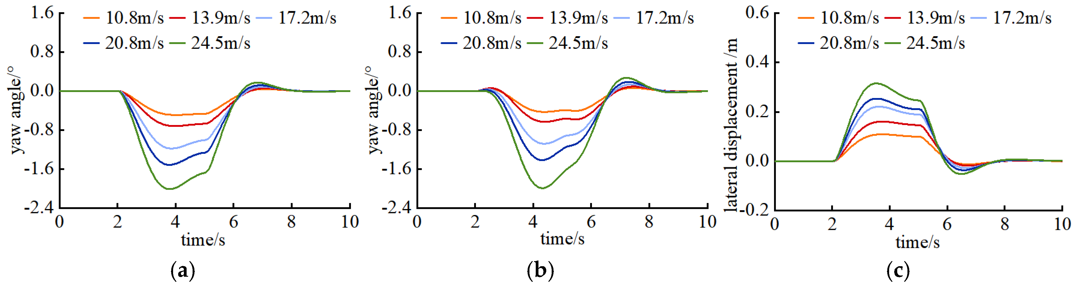
Affected by the saddle of the container truck, the peak moment of the lateral motion and yaw motion responses of the trailer is significantly behind that of the tractor. Although the increase in wind speed will exacerbate the lateral deviation and yaw motion of the container truck, the driver’s feedback operation can effectively control the truck to return to the predetermined straight driving state. The yaw angle of the tractor increases from 0.49° to 2.01° and then gradually becomes stable, while the yaw angle of the semi-trailer increases from 0.43° to 1.99° and gradually becomes stable. The lateral displacement of the truck’s center of mass increases from 0.11 m to 0.31 m and gradually returns to the state of straight driving, as shown in Figure 21. Figure 15 and Figure 16 show that when there is little rainfall, the increase in wind speed has a greater impact on the side wind stability of trucks. The increase in wind speed leads to higher peak lateral acceleration, lateral velocity, yaw angle velocity, and yaw angle for the tractor and semi-trailer. When rainfall reaches 250 mm/h, the road surface adhesion ability becomes smaller, and the change in rainfall has a greater impact on the side wind stability of trucks.

Figure 21.
Skew angle and lateral displacement of container trucks under different wind speeds. (a) Yaw angle of tractor, (b) Yaw angle of semi-trailer, (c) Lateral displacement of centroid.
5. Conclusions
In this study, a container truck was taken as an example to explore the dynamic stability of vehicles under crosswind on sea-crossing bridges with measured wind–rain coupling effects using CFD. The influences of wind speed, wind characteristics, and rain on the aerodynamic force, acceleration, velocity, and yaw angle were numerically investigated. The following conclusions can be made:
- (1)
- To explore wind-induced driving safety under the coupling wind–rain effect on the bridge, an aeroelastic coupling analysis model was established for a cross-sea bridge in a wind and rain environment.
- (2)
- The simulation results show that rainfall significantly affects the top of the truck and the leeward-side flow field and increases the aerodynamic force of the truck on the cross-sea bridge. It also has a more obvious impact on the aerodynamic lift of the semi-trailer.
- (3)
- Truck skidding occurs when rainfall reaches 250 mm/h. With greater rainfall, road surface adhesion capacity is smaller, resulting in a more obvious lateral deviation and yaw movement of the truck and a higher risk of the vehicle sliding.
- (4)
- The crosswind speed significantly increases the aerodynamic force of the truck and enhances the lateral and yaw motion of the tractor and semi-trailer. With the same wind speed, the peak dynamic response of the semi-trailer lags significantly behind that of the tractor.
- (5)
- In general, higher wind speed and turbulence can cause vehicles to experience instability when driving. Considering the measured wind turbulence intensity, the yaw angle peaks of the tractor and trailer increased by 5.2% and 3.8%, respectively, and the lateral displacement of the truck’s center of mass increased by 9.8%.
Generally the wind turbulence intensity and rainfall in coastal areas significantly affect the driving safety of vehicles on sea-crossing bridges. Therefore, when conducting wind stability analyses of vehicles, the weather conditions in coastal areas should be considered to obtain more accurate results and determine more reasonable traffic control strategies in such areas.
Author Contributions
Methodology, D.X., L.L. and Z.Y.; Validation, C.C. and Y.H.; Formal analysis, Z.L.; Investigation, D.X. and C.C.; Data curation, D.X. and L.L.; Writing—original draft, D.X. All authors have read and agreed to the published version of the manuscript.
Funding
This research was funded by the National Natural Science Foundation of China (52278537, 52408558), Fujian Provincial Natural Science Foundation (2022J011251), and High-Level Talent Program of Xiamen University of Technology (YKJ23006R).
Data Availability Statement
The raw data supporting the conclusions of this article will be made available by the authors on request.
Conflicts of Interest
The authors declare no conflicts of interest.
References
- Kim, S.J.; Shim, J.H.; Kim, H.K. How wind affects vehicles crossing a double-deck suspension bridge. J. Wind Eng. Ind. Aerodyn. 2020, 206, 104329. [Google Scholar] [CrossRef]
- Wang, B.; Xu, Y.L. Safety Analysis of a Road Vehicle Passing by a Bridge Tower under Crosswinds. J. Wind Eng. Ind. Aerodyn. 2015, 137, 25–36. [Google Scholar] [CrossRef]
- Chen, F.; Pdeng, H.; Ma, X.; Liang, J.; Hao, W.; Pan, X.D. Examining the safety of trucks under crosswind at bridge-tunnel section: A driving simulator study. Tunn. Undergr. Space Technol. 2019, 92, 103034. [Google Scholar] [CrossRef]
- Li, J.; Gong, R.; Li, J.; Fan, Y.; Huo, Y. Traffic Safety Evaluation Method of Bridge Tunnel Junction Section of Expressway Based on Traffic Simulation. J. Chang. Univ. (Natl. Sci. Ed.) 2023, 43, 82–94. [Google Scholar]
- Sun, M.; Wang, D.; Shen, X.; Chen, A. A Simplified Method for Estimating the Critical Wind Speed of Moving Vehicles on Bridges Under Crosswinds. Int. J. Struct. Stab. Dyn. 2022, 22, 1–28. [Google Scholar] [CrossRef]
- Zhang, J.M.; Ma, C.M.; Xian, R.; Li, J.; Li, Q. Wind Tunnel Investigations of Crosswind Loads for Static Road Vehicles on Wide Bridge Decks. J. Wind Eng. Ind. Aerodyn. 2023, 233, 105315. [Google Scholar] [CrossRef]
- Wang, B.; Wang, W.X.; Li, Y.L.; Lan, F. Aerodynamic Characteristics Study of Vehicle-bridge System Based on Computational Fluid Dynamics. J. Wind Eng. Ind. Aerodyn. 2023, 234, 105351. [Google Scholar] [CrossRef]
- Chen, N.; Li, Y.L.; Wang, B.; Su, Y.; Xiang, H.Y. Effect of wind barrier on the safety of vehicles driven on bridges. J. Wind Eng. Ind. Aerodyn. 2015, 143, 113–127. [Google Scholar] [CrossRef]
- Lin, L.; Chen, K.; Xia, D.; Wang, H.F.; Hu, H.T.; He, F.Q. Analysis on the wind characteristics under typhoon climate at the southeast coast of China. J. Wind Eng. Ind. Aerodyn. 2018, 182, 37–48. [Google Scholar] [CrossRef]
- Shen, H.; Hu, W.; Yang, Q.; Yang, F.; Guo, K.; Zhou, T.; Qian, G.; Xu, Q.; Yuan, Z. Non-Gaussian wind features over complex terrain under atmospheric turbulent boundary layers: A case study. Wind Struct. 2022, 35, 419–430. [Google Scholar]
- Li, Y.L.; Xu, X.; Zhang, M.J.; Xu, Y.L. Wind tunnel test and numerical simulation of wind characteristics at a bridge site in mountainous terrain. Adv. Struct. Eng. 2017, 20, 1223–1231. [Google Scholar] [CrossRef]
- Song, J.; Li, J.W.; Xu, R.; Flay, R. Field Measurements and CFD Simulations of Wind Characteristics at the Yellow River Bridge Site in a Converging-channel Terrain. Eng. Appl. Comput. Fluid Mech. 2022, 16, 58–72. [Google Scholar] [CrossRef]
- Wang, J.; Li, J.; Wang, F. Research on Wind Field Characteristics Measured by Lidar in a U-Shaped Valley at a Bridge Site. Appl. Sci. 2021, 11, 9645. [Google Scholar] [CrossRef]
- Yu, M.; Liu, J.; Dai, Z. Aerodynamic Characteristics of a High-speed Train Exposed to Heavy Rain Environment Based on Non-spherical Raindrop. J. Wind Eng. Ind. Aerodyn. 2021, 211, 104532. [Google Scholar] [CrossRef]
- Yu, M.; Li, M.; Liu, J. Liquid film morphology and aerodynamic performance of a high-speed train under wind-rain environments. J. Wind Eng. Ind. Aerodyn. 2024, 247, 105687. [Google Scholar] [CrossRef]
- Zeng, G.; Li, Z.; Huang, S. Aerodynamic Characteristics of Intercity Train Running on Bridge under Wind and Rain Environment. Alex. Eng. J. 2023, 66, 873–889. [Google Scholar] [CrossRef]
- Yuan, Z.; Gu, Z.; Wang, Y.; Huang, X. Numerical investigation for the influence of the car underbody on aerodynamic force and flow structure evolution in crosswind. Adv. Mech. Eng. 2018, 10, 1687814018797506. [Google Scholar] [CrossRef]
- T/CSAE 112-2019; Technical Specification of Passenger Car Aerodynamic Numerical Simulation. Chinese Society of Automotive Engineers: Beijing, China, 2019.
- Best, A.C. The Size Distribution of Raindrop. Q. J. R. Meteorol. Soc. 1950, 76, 16–36. [Google Scholar] [CrossRef]
- Ulbrich, C.W. Natural Variations in the Analytical Form of the Raindrop Size Distribution. J. Clim. Appl. Meteorol. 1983, 22, 1764–1775. [Google Scholar] [CrossRef]
- Gunn, R. The Free Electrical Charge on Thunderstorm Rain and Its Relation to Droplet Size. J. Geophys. Res. 1949, 54, 57–63. [Google Scholar] [CrossRef]
- Gunn, R.; Kinzer, G.D. The Terminal Fall Velocity for Water Droplets in Stagnant Air. J. Atmos. Sci. 1949, 6, 243–248. [Google Scholar] [CrossRef]
- Yuan, Z.; Xia, D.; Lin, X.; Lin, L.; Liu, Y.; Li, Y. Influence Mechanism of a Bridge Wind Barrier on the Stability of a Van-Body Truck under Crosswind. Atmosphere 2022, 13, 360. [Google Scholar] [CrossRef]
- Ji, T.; Huang, X.; Liu, Q.; Tang, G. Asphalt pavement surface water film thickness test. Highw. Traffic Sci. Technol. 2004, 21, 14–17. (In Chinese) [Google Scholar]
- Ji, T.; Huang, X.; Liu, Q. Part Hydroplaning Effect on Pavement Friction Coefficient. J. Transp. Eng. 2003, 3, 10–12. (In Chinese) [Google Scholar]
Disclaimer/Publisher’s Note: The statements, opinions and data contained in all publications are solely those of the individual author(s) and contributor(s) and not of MDPI and/or the editor(s). MDPI and/or the editor(s) disclaim responsibility for any injury to people or property resulting from any ideas, methods, instructions or products referred to in the content. |
© 2025 by the authors. Licensee MDPI, Basel, Switzerland. This article is an open access article distributed under the terms and conditions of the Creative Commons Attribution (CC BY) license (https://creativecommons.org/licenses/by/4.0/).