Investigation of Driving Safety on Desert Highways Under Crosswind Direction Disturbances

Abstract

Desert highways, with open terrain and minimal wind barriers, expose high-speed vehicles to significant stability risks from combined crosswinds and sand accumulation. This study uses numerical simulation to assess the effects of varying wind direction angles and sand thicknesses on vehicle stability across different models. Five dynamic indicators—lateral displacement, yaw angle, aerodynamic sideslip angle, lateral acceleration, and roll angle—are analyzed. The results show that a 120° wind angle causes the most pronounced parameter changes, while stability is lowest at 150°, where critical thresholds are reached within 0.75 s and danger thresholds by 2.25 s. Rapid wind speed variations further degrade stability. Compared to small SUVs, mid-size SUVs perform worse under identical conditions. A comprehensive stability evaluation function is proposed to quantify the combined impact of wind angle and surface friction, providing a new approach for safety assessment on sand-covered desert roads.

1. Introduction

In desert regions, the terrain is vast and flat, vegetation is sparse, climatic conditions are extreme, and large areas of the ground surface are exposed to loose sand. Highways traversing these areas are frequently subjected to complex environmental factors such as strong crosswinds, drastic temperature fluctuations, and sand accumulation on the road surface, all of which pose serious threats to driving safety [1]. Strong crosswinds can significantly impair a vehicle’s lateral stability and yaw control, increasing the risk of lane departure or rollover. Meanwhile, variations in sand thickness alter road surface friction characteristics, reducing braking and handling performance and increasing driving difficulty. Therefore, investigating the combined effects of crosswinds and sand accumulation is crucial for improving driving safety on desert highways and optimizing vehicle safety design.

The crosswind effect on desert highways is one of the critical factors affecting vehicle driving safety. Under crosswind conditions, the vehicle’s dynamic response is mainly manifested as lateral displacement, body roll, and steering instability, which may even lead to rollover accidents [2]. Current research on the impact of crosswinds on vehicle safety primarily relies on wind tunnel experiments and numerical simulations. Wind tunnel testing includes both scaled model tests and full-scale vehicle tests. Yang et al. [3] investigated the aerodynamic characteristics of a passenger car passing over a sand dune under crosswind conditions by comparing three turbulence models: RNG k–ε, LES, and IDDES. The results showed that the LES model yielded the best agreement with experimental data in predicting aerodynamic loads, with an error range of 4.4–7.5%, providing a valuable numerical reference for vehicle safety in desert environments. Gohlke et al. [4] demonstrated through 1:5 scale wind tunnel tests that even slight changes in A-pillar radius significantly affect side force and yaw moment, which are closely related to the formation and intensity of A-pillar vortices. Cheli et al. [5] investigated the lateral force admittance function of heavy vehicles through wind tunnel experiments and found that side area is the dominant influencing factor. Although wind tunnel tests are cost-effective and flexible, they are constrained by scaling effects. In contrast, full-scale vehicle tests offer higher accuracy but involve greater cost. Brandt et al. [6] employed a one-dimensional numerical coupling approach in combination with vehicle dynamics models of varying complexity to analyze the effects of crosswinds on vehicle stability. Their study identified key influencing factors and showed that medium-complexity models can effectively capture vehicle response, providing valuable references for the optimization of crosswind stability design.

With the advancement of technology, numerical simulation methods have gradually become the primary tool for studying the impact of crosswinds on vehicle safety, compensating for the limitations of wind tunnel testing. Numerical simulations offer advantages such as low cost, high flexibility, rich detail, and the absence of scaling effects. Tsubokura et al. [7] and Huang et al. [8,9,10] employed large eddy simulation (LES) to investigate the influence of vehicle geometry on the unsteady dynamic response to crosswinds. LES filters large- and small-scale motions in the flow field, directly computing large-scale vortex behavior while modeling small-scale vortices. Compared to traditional turbulence models (e.g., Reynolds-averaged Navier–Stokes equations [11]), LES retains more flow details and is suitable for predicting transient and complex flows. However, due to its high computational resource demand, complex wall treatment, and potential instability, LES has limitations for widespread application. Liu et al. [12] proposed a vehicle stability control strategy based on dynamic stability region regression analysis, employing support vector regression (SVR) and linear time-varying model predictive control (LTV-MPC). The approach significantly improved vehicle stability and braking performance under various driving conditions. Ekman et al. [13] employed the RANS-LES hybrid method, using RANS near the wall and LES further from the wall to improve simulation accuracy. Wang et al. [14] used the unsteady Reynolds-averaged Navier–Stokes (URANS) method, combining CFD and multibody dynamics, to study the effects of crosswinds on vehicle safety, validated by a 1:3 scale model wind tunnel test. URANS can capture transient changes at lower costs. Yang and Tian [15] proposed an adaptive cruise control strategy that integrates fuzzy model predictive control with sliding mode control, achieving coordinated optimization of longitudinal following performance and lateral stability. Koysuren et al. [16] proposed a physics-informed deep-learning-based online parameter estimation method, which enables efficient and accurate identification of front and rear cornering stiffness under limited sensor data, thereby enhancing the tracking performance of the control system under varying driving conditions. Fu [17] examined the relationship between drag coefficient and vehicle safety, while Taiming et al. [18] explored the effect of crosswinds on vehicle aerodynamic stability under different road surface coefficients. Brandt [19] used aerodynamics and vehicle dynamics coupling simulations, combining experimental and numerical methods, to study the effect of crosswinds on passenger car stability. They found that yaw moment overshoot was related to flow field phase delay and identified aerodynamic yaw moment coefficient and center of gravity position as core influencing factors. Yang et al. [20], based on the Xihumen Bridge, studied the impact of strong crosswinds on the bridge deck wind environment and driving safety, proposing an adjustable wind barrier solution to reduce deck wind speed and optimize the anti-vortex excitation performance of the main girder. Zhang et al. [21] investigated the impact of complex wind environments in canyon–bridge–tunnel sections on sedan stability, proposing an aerodynamics–vehicle dynamics coupling method combined with GIS and numerical simulation to analyze the impact of terrain on vehicle aerodynamic characteristics, providing theoretical support for vehicle stability assessment in complex terrains.

In conclusion, existing studies have primarily focused on the effects of crosswinds on different vehicle types, using various methods such as wind tunnel testing and numerical simulations. Many studies have investigated the lateral stability, yaw characteristics, and aerodynamic response of passenger cars, heavy vehicles, and other types of vehicles under crosswind conditions, proposing strategies to optimize aerodynamic design and reduce the impact of crosswinds. However, most of the existing research has concentrated on urban roads, bridges, and other complex terrains. There is a lack of systematic research on the impact of crosswinds and sand accumulation on vehicle safety in desert regions. Therefore, conducting research on the effects of crosswinds on vehicle safety in desert highways is of significant practical importance.

This study combines the six-degree-of-freedom theory and uses CarSim to simulate the dynamic response of SUV vehicles under different wind speeds, wind direction angles, and sand accumulation thickness conditions, exploring their driving safety on desert highways. After excluding the interference of driver operation variables, five dynamic indicators—offset, yaw angle, aerodynamic sideslip angle, acceleration, and roll angle—are introduced to systematically investigate the effects of different combinations of wind direction angles and road surface friction coefficients on vehicle safety under instantaneous constant wind speeds, using a comprehensive stability evaluation function for quantitative analysis. The research results provide a reference for improving vehicle driving safety on desert highways.

2. Model Construction

Currently, commonly used vehicle simulation software includes CarSim2020 and Simulink2023a. Among them, CarSim2020 is widely used in vehicle stability studies under complex conditions such as crosswinds due to its convenient modeling, fast simulation speed, strong visualization capabilities, and modular interfaces for the vehicle body, tires, and aerodynamics, as shown in Figure 1.

Under strong crosswind conditions, vehicles are not only at risk of path deviation, but also face safety issues such as loss of posture control, handling difficulty, and rollover. To comprehensively evaluate the impact of crosswinds on vehicle stability, this study selects five key dynamic indicators: lateral displacement, yaw angle, aerodynamic sideslip angle, lateral acceleration, and roll angle. These indicators encompass three aspects of vehicle response under crosswind—path deviation, attitude change, and dynamic stability. They are physically meaningful and highly complementary, enabling the construction of a systematic and comprehensive stability evaluation framework, as shown in Figure 2 and Figure 3.

2.1. Vehicle Modeling

Vehicles traveling on desert highways are predominantly SUVs, as they typically feature higher ground clearance compared to smaller cars. This design helps prevent contact between the chassis and sand, reducing the risk of becoming stuck and providing greater traction. In this study, two representative SUV models are selected: the small SUV Geely Binyue and the mid-size SUV Chery Tiggo 8 (2024 edition). Their key specifications are listed in

Table 1. Vehicle technical model parameters.

Parameter	Small SUV	Mid-Size SUV
Length × Width × Height (mm)	4300 × 1800 × 1609	4700 × 1860 × 1746
Wheelbase (mm)	2600	2710
Front Track/Rear Track (mm)	1551/1600	1582/1604
Frontal Area (m2)	3.7	3.9
Vehicle Weight (kg)	1340	1509
Unsprung Mass (kg)	1139	1283
Tire Model	215/55 R17	235/55 R18
Ixx (kg·m2)	474.1	619.7
Iyy (kg·m2)	2169.5	2858.2
Izz (kg·m2)	2451.2	2975.5
Center of Gravity Height (mm)	642	666
COG Longitudinal Position (from front axle)	1101	1148

.

2.2. Wind Speed Configuration

In desert regions, short-duration crosswind events—typically lasting 2 to 3 s with relatively stable wind speed and direction—are frequently observed. Although these are not classified as sustained strong winds, they can significantly impair vehicle stability, increasing the risk of lateral deviation, sideslip, or even rollover.

To replicate such typical gust scenarios, this study applies a steady crosswind input of 17.1 m/s lasting 3 s. This value corresponds to the maximum wind speed within Level 7 wind as defined by China’s national standard [22] Wind Force Classification, and is also one of the most frequently recorded wind levels on desert highways, particularly in regions such as Alxa, Inner Mongolia. The 3-s duration reflects the average time required for a vehicle to pass through a localized gust disturbance zone, based on both field observations and prior research. This parameter setting ensures the simulation is both realistic and repeatable, while maintaining computational controllability.

The aerodynamic load due to crosswind is applied with a wind pressure center height of 1.2 m and an air density of 1.206 kg/m³, corresponding to standard atmospheric conditions (20 °C, 101.3 kPa). While actual desert temperatures and pressures may deviate slightly, their overall influence on aerodynamic force computation is limited, making the chosen values physically reasonable. The selected pressure center height approximates the location of the vehicle’s aerodynamic center or center of gravity and aligns with general vehicle design practices.

Although direct experimental validation under desert-specific conditions is not available, the baseline response of the CarSim model under crosswind was compared with published wind tunnel test results for a similar mid-size passenger car [23,24,25]. The predicted lateral displacement and yaw rate trends showed good agreement, supporting the credibility and engineering applicability of the simulation model.

2.3. Driving Mode Settings

This study uses the open-loop driving control mode in CarSim to eliminate the influence of driver intervention on the vehicle’s dynamic response, aiming to more accurately reflect the actual and critical safety conditions of driving on desert highways. For this purpose, a vehicle speed of 100 km/h is selected as the typical operating condition, which aligns with the speed limit on high-grade highways in desert regions of China and represents the speed range at which medium and small vehicles are most sensitive to crosswind disturbances. This speed setting effectively identifies the impact of factors such as wind speed, wind direction, and sand accumulation on vehicle stability, and holds representational and engineering reference value. In this mode, the vehicle maintains a constant throttle, engine braking, or braking, with the transmission in neutral and the steering wheel kept at 0 degrees, as shown in Figure 4. It is primarily used to study the effects of external disturbances (such as crosswind, sand accumulation, etc.) on vehicle stability, making it suitable for verifying the stability boundaries under passive responses.

2.4. Road Settings

In this study, data on sand accumulation thickness on desert highways were collected through field tests. According to the measured data, the sand accumulation thickness is closely related to the desert crosswind. Strong winds carry sand particles to the road surface, where they accumulate to form a sand layer. To further quantify this process, a pendulum friction tester was used to measure the friction coefficient of the sand layer. The relationship between sand accumulation thickness and the friction coefficient is shown in Figure 5.

Based on the results shown in Figure 5, the relationship between sand accumulation thickness and road surface friction coefficient exhibits a trend of first decreasing and then increasing, with the change becoming more gradual in the later stages. The friction coefficient at a sand accumulation thickness of 6 mm corresponds to the lowest point. Therefore, in the simulation, the road section is set as a straight line, with the no-sand surface and the surface with a sand accumulation thickness of 6 mm selected as control groups, having friction coefficients of 0.9584 and 0.8030, respectively. This setup will help analyze the effect of sand accumulation thickness on the friction coefficient and provide data support for further research.

The sand thickness was set to two representative levels: 0 mm (clean road surface) and 6 mm (severe accumulation), with 6 mm corresponding to the maximum value observed in field measurements. Preliminary tests using a British Pendulum Tester indicated that intermediate values (2–4 mm) result in minimal changes in surface friction, suggesting limited influence on vehicle dynamics. Therefore, the use of boundary conditions is sufficient to evaluate the impact of sand accumulation in a conservative and representative manner.

3. Simulation Results and Analysis

3.1. Impact of Different Wind Direction Angles on Driving Safety

In the wind direction angle analysis, this study examined the stability performance of a small SUV and a medium SUV at wind direction angles of 30°, 60°, 90°, 120°, and 150°, considering two conditions: 0 mm and 6 mm sand thickness. During the simulation, the vehicle speed was set to 100 km/h, the wind speed was 17.1 m/s, the data step size was 0.25 s, and the simulation duration was 3 s.

3.1.1. Effect of Wind Direction on Driving Safety Without Sand

As shown in Figure 6, under the conditions of a vehicle speed of 100 km/h and wind speed of 17.1 m/s, the lateral displacement of the small SUV increases with the wind direction angle, following the sequence of 30°, 60°, 150°, 90°, and 120°. Notably, the rate of increase in lateral displacement becomes faster at a wind direction of 150°, eventually approaching the displacement caused by a 90° wind direction. This trend is also reflected in the yaw angle, where, in the initial state, the sequence of the yaw angle corresponds to that of lateral displacement. However, at 1.5 s, the yaw angle induced by the 150° wind direction exceeds that caused by the 90° wind direction. In terms of aerodynamic slip angle, it decreases with the increase in wind direction angle, with the 60° wind direction becoming the most influential over time. Meanwhile, the lateral acceleration and roll angle are predominantly affected by the 120° wind direction.

As shown in Figure 7, at a speed of 100 km/h and wind speed of 17.1 m/s, the five indicators of the medium SUV exhibit similar trends to the small SUV, with slightly higher values.

3.1.2. Impact of Crosswind on Driving Safety with Sand on the Road

Figure 8 shows the variation in various indicators of the small SUV with wind direction angles at a speed of 100 km/h and a wind speed of 17.1 m/s, when the sand thickness is 6 mm. Although the values are slightly higher, the overall trend remains similar to that observed with a sand thickness of 0 mm.

Figure 9 shows that under the conditions of a sand thickness of 6 mm, a vehicle speed of 100 km/h, and a wind speed of 17.1 m/s, the variation in various indicators for the medium SUV with wind direction angle follows the same trend as that with a sand thickness of 0 mm, with a slight increase in values.

Figure 6, Figure 7, Figure 8 and Figure 9 show that a wind direction angle of 120° has the most significant impact on the vehicle’s lateral displacement and yaw angle. The medium SUV, due to its larger frontal area and higher center of gravity, is more affected by the wind, requiring more frequent steering corrections and increasing driver fatigue. When evaluating the effect of wind on yaw angle, at low wind speeds, the 120° wind direction causes the largest yaw angle, while the yaw rate caused by a 150° wind direction increases, indicating that higher wind speeds enhance the rear vortex, leading to increased yaw moment. This effect is more pronounced in rear disturbances, which can negatively impact vehicle stability. At high wind speeds, rear flow separation intensifies, causing the vehicle’s rear to be more easily displaced. As the wind direction angle increases, the aerodynamic slip angle decreases as the crosswind effect becomes more parallel to the vehicle body, reducing lateral interference. Lateral acceleration increases with wind direction angle, with the most notable effect at a 120° wind direction. Due to the sensitivity of acceleration to crosswinds, wind forces immediately induce nonlinear changes in acceleration, resulting in instantaneous aerodynamic disturbances followed by delayed dynamic responses. This behavior is especially prominent during the initial phase of crosswind, where the vehicle is most unstable, posing a significant safety risk. Roll angle increases with the wind direction angle, particularly at 120°, where the crosswind is nearly perpendicular to the vehicle’s direction of motion. This generates the maximum lateral and rolling moments, making the vehicle more prone to tipping or losing control, thus increasing rollover risk.

3.2. Sand Accumulation Thickness

The sand carried by crosswinds adheres to the road surface, altering its friction coefficient. This section analyzes the impact of road surface friction—measured experimentally at 0 mm and 6 mm sand thickness—on driving safety. Final results are obtained through 3-s simulations using CarSim.

Table 2. Variation in lateral displacement with sand accumulation thickness.

Vehicle Type	Lateral Displacement (m)
	0 mm					6 mm
	30°	60°	90°	120°	150°	30°	60°	90°	120°	150°
Small SUV	0.9145	2.9091	6.0709	7.8982	5.8264	0.9145	2.9091	6.0714	7.8993	5.8264
Medium SUV	1.1343	3.5113	6.9577	8.8755	6.5615	1.1343	3.5113	6.9586	8.8764	6.5615

,

Table 3. Variation in yaw angle with sand accumulation thickness.

Vehicle Type	Yaw Angle (deg)
	0 mm					6 mm
	30°	60°	90°	120°	150°	30°	60°	90°	120°	150°
Small SUV	1.0221	3.2976	7.5073	10.5460	8.2877	1.0221	3.2976	7.5076	10.5468	8.2877
Medium SUV	1.3673	4.2428	8.9677	12.2962	9.7120	1.3673	4.2428	8.9684	12.2970	9.7120

,

Table 4. Variation in aerodynamic sideslip angle with sand accumulation thickness.

Vehicle Type	Aerodynamic Slip Angle (deg)
	0 mm					6 mm
	30°	60°	90°	120°	150°	30°	60°	90°	120°	150°
Small SUV	46.4856	47.3517	40.4743	30.5897	17.0078	46.4856	47.3517	40.4744	30.5900	17.0078
Medium SUV	46.4224	47.5637	41.0015	31.3490	17.6813	46.4224	47.5637	41.0018	31.3493	17.6813

,

Table 5. Variation in acceleration with sand accumulation thickness.

Vehicle Type	Lateral Accel. of CGs (g)
	0 mm					6 mm
	30°	60°	90°	120°	150°	30°	60°	90°	120°	150°
Small SUV	0.0161	0.0486	0.1064	0.1553	0.1342	0.0161	0.0486	0.1064	0.1553	0.1342
Medium SUV	0.0222	0.0644	0.1300	0.1853	0.1623	0.0222	0.0644	0.1300	0.1853	0.1623

and

Table 6. Variation in roll angle with sand accumulation thickness.

Vehicle Type	Roll Angle of Sprung Masses (deg)
	0 mm					6 mm
	30°	60°	90°	120°	150°	30°	60°	90°	120°	150°
Small SUV	−0.2139	−0.7320	−1.2461	−1.3735	−0.9198	−0.2139	−0.7320	−1.2461	−1.3735	−0.9198
Medium SUV	−0.1796	−0.6418	−1.1063	−1.2267	−0.8360	−0.1796	−0.6418	−1.1063	−1.2267	−0.8360

present the variations in key indicators at 3 s under different sand accumulation thicknesses and crosswind directions. The results show that sand accumulation thickness has a relatively minor impact on these indicators, with many values converging. This suggests that sand thickness is a secondary factor in influencing driving stability. In desert highway environments, crosswinds remain the dominant external disturbance, exerting a much greater influence on vehicle dynamic responses than the changes in surface friction caused by sand. Moreover, within the tested range of sand thicknesses, the variation in road surface friction coefficient is limited and does not significantly impair vehicle stability. Additionally, the vehicle’s dynamic model demonstrates a degree of robustness to slight friction fluctuations, and no severe skidding or loss of control was observed in the simulations, further diminishing the effect of sand thickness on critical performance indicators. Therefore, in strong crosswind conditions, wind speed and direction remain the primary factors affecting vehicle stability.

3.3. Evaluation Method

In this study, a comprehensive stability evaluation function was introduced to establish a unified assessment standard across multiple indicators. This method not only enhances the objectivity and comparability of the evaluation but also helps reveal the overall trends in vehicle response, thereby avoiding biased judgments that may result from relying on a single indicator.

$$S\left(h\right)={\displaystyle \sum }_{i=1}^n{w}_i·{\displaystyle \frac{x_i\left(\mu \left(h\right)\right)}{x_{i,max}}}$$

(1)

In the equation, $x_i\left(\mu \left(h\right)\right)$ represents the value of the i stability indicator under the condition corresponding to the friction coefficient μ; $x_{i,max}$ denotes the critical (threshold) value of the indicator under unstable conditions; $w_i$ represents the weight assigned to each indicator. The smaller the overall result, the better the stability—values closer to 1 indicate a higher level of danger.

Use the CRITIC method to assign values to the weights of each indicator.

Perform range normalization on each indicator to make the data dimensionless:

$$x^{\prime }={\displaystyle \frac{x-\min \left(x\right)}{\max \left(x\right)-\min \left(x\right)}}$$

(2)

Calculate the Pearson correlation coefficient $r_{ij}$:

$$r_{ij}={\displaystyle \frac{{\displaystyle \sum _{k=1}^n(x_{ik}^{’}-\overline{x_i})(x_{jk}^{’}-\overline{x_j})}}{(\mathrm{n}-1){\mathrm{S}}_{\mathrm{i}}{\mathrm{S}}_{\mathrm{j}}}}$$

(3)

In the formula, $x_{ik}^{’}$ and $x_{jk}^{’}$ represent the values of the i and j indicators for the k sample on the i and j indicators, respectively. $\overline{x_i}$ and $\overline{x_j}$ represent the mean values of the i and j indicators. ${\mathrm{S}}_{\mathrm{i}}$ represents the sample standard deviation of the i indicator, where the denominator is n − 1, with n being the number of samples. The sample standard deviation is used here instead of the population standard deviation because the simulation uses sample values extracted at a step size of 0.25 s rather than all the data, so the sample standard deviation better reflects the data’s dispersion.

The Pearson correlation coefficient ranges from −1 to 1, indicating the degree of linear correlation between two indicators. A value closer to 1 indicates a stronger correlation between the two indicators, while a value closer to 0 suggests no linear correlation between the indicators.

Calculate the standard deviation for each indicator:

$${\sigma }_j=\sqrt{{\displaystyle \frac{1}{n-1}}{\displaystyle \sum _{\mathrm{i}=1}^N{(x_i-\overline{x})}^2}}$$

(4)

In the formula, ${\sigma }_j^2$ is the standard deviation, N is the number of data points in the dataset, $x_i$ represents each data point in the dataset, and $\overline{x}$ is the mean of the dataset.

Next, the adjusted standard deviation is calculated, which accounts for the influence of other indicators. This step is carried out by computing the correlation of each indicator with the others and then adjusting the standard deviation accordingly.

$${\sigma }_i^{adj}={\sigma }_i\sqrt{1-{\displaystyle \frac{1}{n-1}}{\displaystyle \sum _{j\ne i}{r}_{ij}^2}}$$

(5)

In the formula, $r_{ij}$ represents the correlation between the i and j indicators. ${\displaystyle \sum _{j\ne i}{r}_{ij}^2}$ is the sum of the squared correlation coefficients between the i indicator and all other indicators.

Finally, the weight of each indicator is calculated based on its standard deviation and its correlation with other indicators. The CRITIC method defines the weight using the following formula:

$$w_i={\displaystyle \frac{{\sigma }_i^{adj}}{{{\displaystyle \sum }}_{i=1}^{\mathrm{m}}{\sigma }_i^{adj}}}$$

(6)

Next, the comprehensive stability evaluation function is calculated.

$$S_i={\displaystyle \sum }_{j=1}^n{w}_j·x_{ij}$$

(7)

The stability function is averaged to represent the average instability level of the entire operating condition.

$$S_{avg}={\displaystyle \frac{1}{n}}{\displaystyle \sum }_{i=1}^{13}{S}_i$$

(8)

In the equation, $n$ represents the number of operating conditions. Take the maximum value to represent the most dangerous moment for the vehicle under that wind direction angle.

$$S_{max}=\max \left(S_1,S_2\dots ,S_n\right)$$

(9)

From

Table 7. Stability levels of a small SUV at different wind angles with 0 mm sand coverage.

Time (s)	30° Wind Heading	60° Wind Heading	90° Wind Heading	120° Wind Heading	150° Wind Heading
0	0.575	0.585	0.594	0.593	0.588
0.25	0.236	0.246	0.233	0.212	0.236
0.5	0.234	0.246	0.267	0.295	0.353
0.75	0.243	0.252	0.269	0.295	0.361
1	0.253	0.260	0.271	0.292	0.361
1.25	0.265	0.271	0.279	0.299	0.371
1.5	0.279	0.285	0.291	0.310	0.386
1.75	0.296	0.300	0.305	0.323	0.402
2	0.314	0.319	0.322	0.339	0.422
2.25	0.335	0.339	0.341	0.357	0.443
2.5	0.358	0.361	0.363	0.377	0.468
2.75	0.383	0.386	0.386	0.400	0.494
3	0.410	0.412	0.412	0.425	0.523
Savg	0.322	0.328	0.333	0.348	0.416
Smax	0.575	0.585	0.594	0.593	0.588

,

Table 8. Stability levels of a midsize SUV at different wind angles with 0 mm sand coverage.

Time (s)	30° Wind Heading	60° Wind Heading	90° Wind Heading	120° Wind Heading	150° Wind Heading
0	0.562	0.578	0.593	0.601	0.559
0.25	0.223	0.234	0.218	0.207	0.213
0.5	0.216	0.233	0.262	0.325	0.360
0.75	0.239	0.254	0.295	0.378	0.431
1	0.259	0.269	0.302	0.380	0.440
1.25	0.274	0.280	0.305	0.376	0.443
1.5	0.289	0.292	0.311	0.380	0.455
1.75	0.306	0.307	0.323	0.391	0.474
2	0.326	0.326	0.337	0.404	0.496
2.25	0.349	0.346	0.354	0.420	0.519
2.5	0.374	0.369	0.374	0.437	0.545
2.75	0.401	0.395	0.396	0.457	0.573
3	0.431	0.422	0.420	0.479	0.603
Savg	0.327	0.331	0.345	0.403	0.470
Smax	0.562	0.578	0.593	0.601	0.603

,

Table 9. Stability levels of a small SUV at different wind angles with 6 mm sand coverage.

Time (s)	30° Wind Heading	60° Wind Heading	90° Wind Heading	120° Wind Heading	150° Wind Heading
0	0.575	0.585	0.594	0.593	0.588
0.25	0.236	0.246	0.234	0.212	0.236
0.5	0.234	0.246	0.267	0.295	0.353
0.75	0.243	0.252	0.269	0.295	0.361
1	0.253	0.260	0.271	0.292	0.361
1.25	0.265	0.271	0.279	0.299	0.371
1.5	0.279	0.285	0.291	0.310	0.386
1.75	0.296	0.300	0.305	0.323	0.402
2	0.314	0.319	0.322	0.338	0.422
2.25	0.335	0.339	0.341	0.357	0.443
2.5	0.358	0.361	0.363	0.377	0.468
2.75	0.383	0.386	0.386	0.400	0.494
3	0.410	0.412	0.412	0.425	0.523
Savg	0.322	0.328	0.333	0.347	0.416
Smax	0.575	0.585	0.594	0.593	0.588

and

Table 10. Stability levels of a medium SUV at different wind angles with 6 mm sand coverage.

Time (s)	30° Wind Heading	60° Wind Heading	90° Wind Heading	120° Wind Heading	150° Wind Heading
0	0.562	0.578	0.593	0.601	0.559
0.25	0.223	0.234	0.218	0.207	0.213
0.5	0.216	0.233	0.262	0.325	0.360
0.75	0.239	0.254	0.295	0.378	0.431
1	0.259	0.269	0.302	0.380	0.440
1.25	0.274	0.280	0.305	0.376	0.443
1.5	0.289	0.292	0.311	0.380	0.455
1.75	0.306	0.307	0.323	0.391	0.474
2	0.326	0.326	0.337	0.404	0.496
2.25	0.349	0.346	0.354	0.420	0.519
2.5	0.374	0.369	0.374	0.437	0.545
2.75	0.401	0.395	0.396	0.457	0.573
3	0.431	0.422	0.420	0.478	0.603
Savg	0.327	0.331	0.345	0.403	0.470
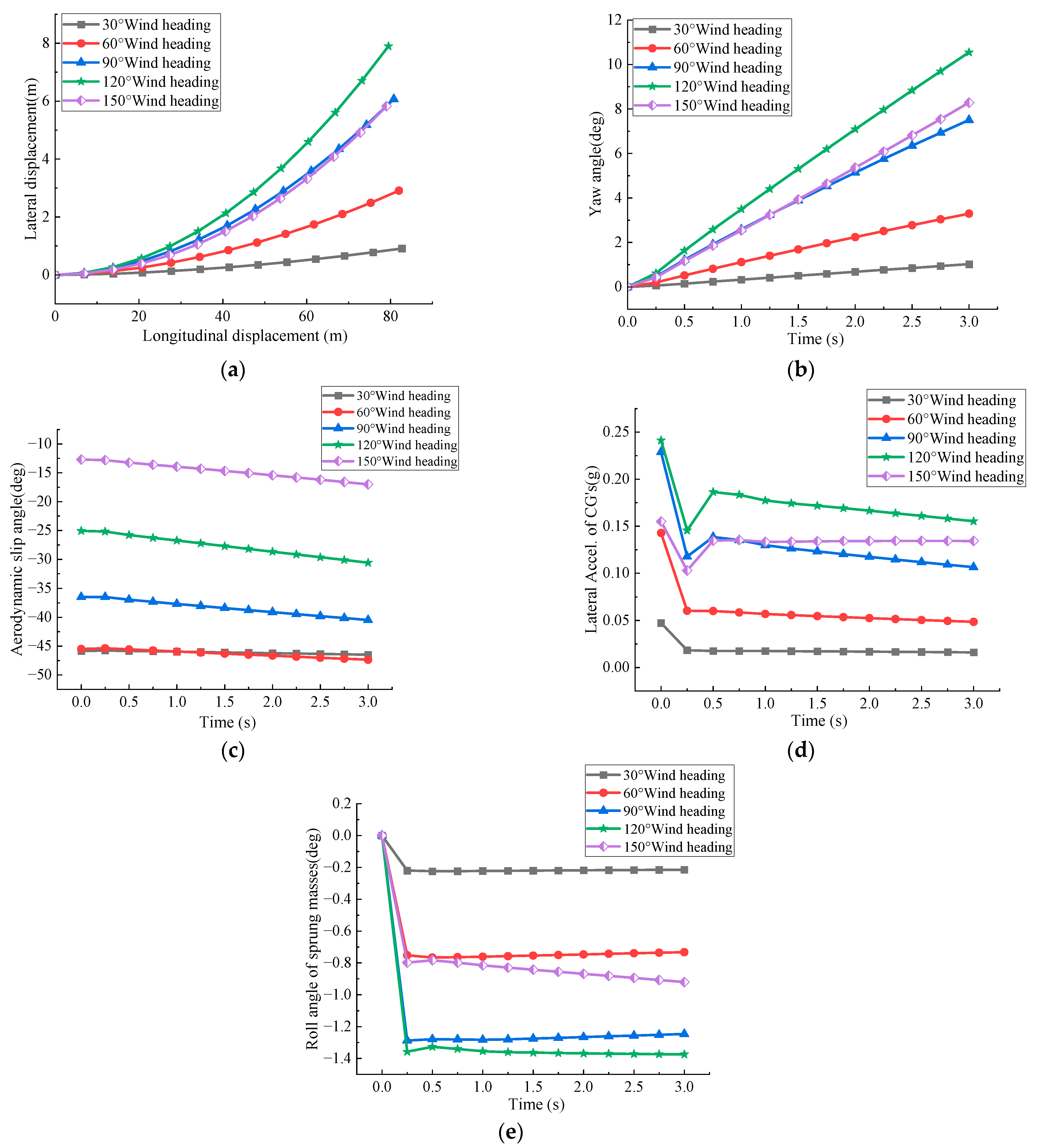
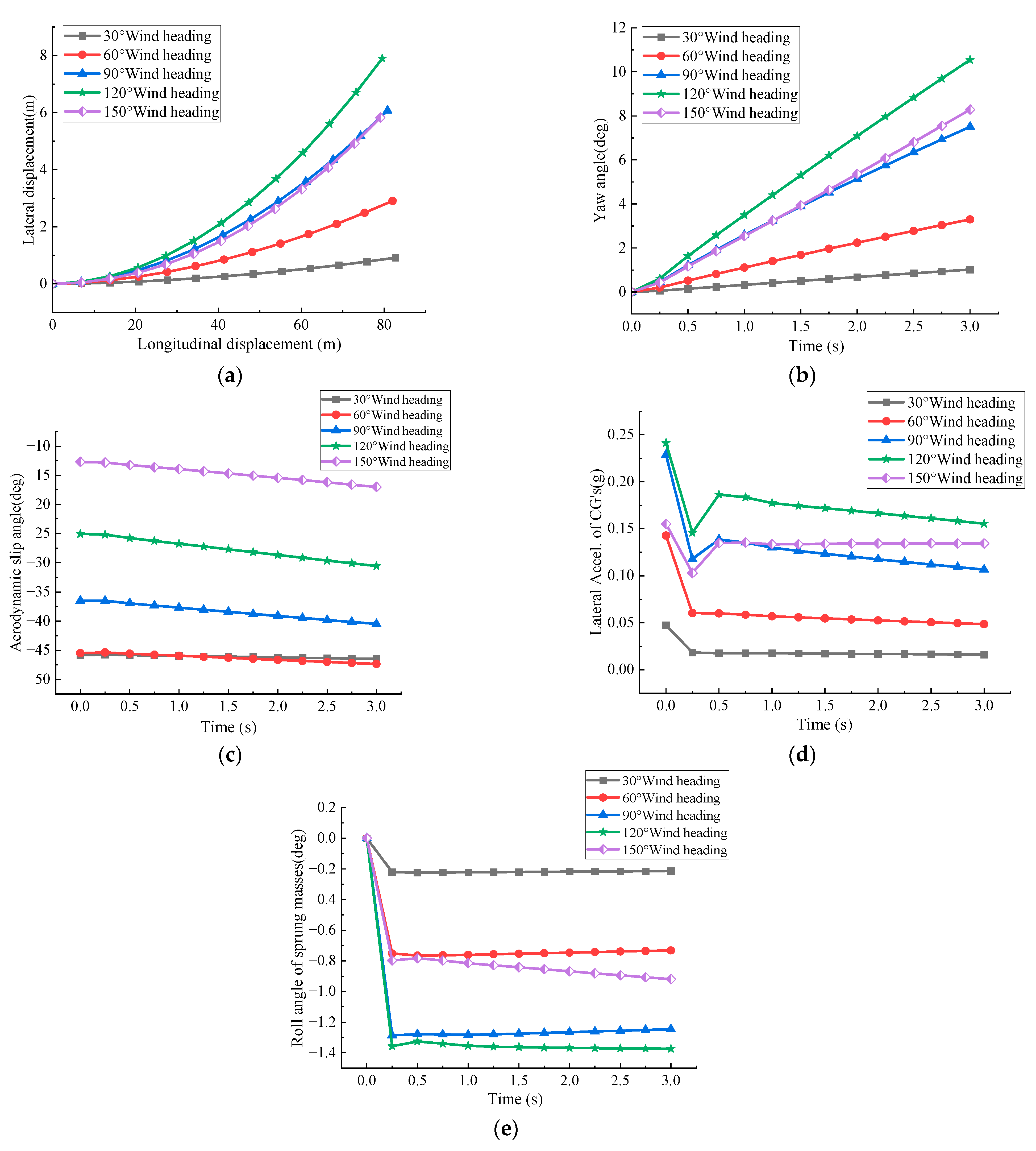
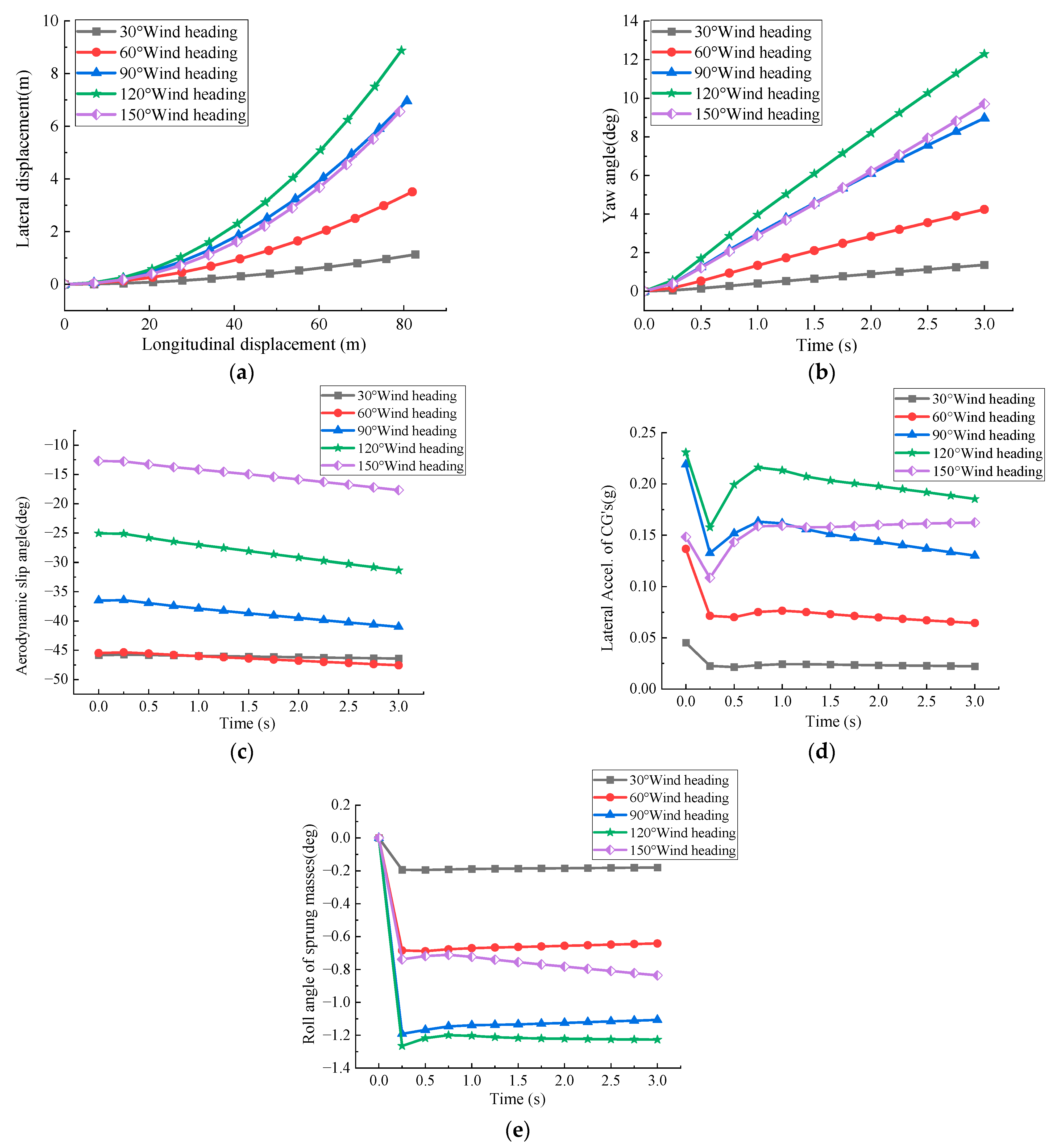
Smax	0.562	0.578	0.593	0.601	0.603

, it can be observed that the vehicle stability is worst at the beginning (0 s), then decreases, and as the wind angle increases, the stability deteriorates again. This is a normal phenomenon. In reality, it manifests as sudden vehicle shaking followed by gradual drifting. The reason is that the vehicle experiences an external disturbance suddenly, entering an unstable state due to a lack of response and inertia. Over time, and with changes in wind direction, the vehicle initially recovers stability, but as external disturbances (increasing wind angle) increase, the stability deteriorates again. The increase in sand thickness does not significantly affect vehicle stability.

There are differences in the instability performance of the vehicle at different wind angles. In most cases, the maximum instability occurs at the moment when the crosswind first acts (0 s), but at a 150° wind angle, the peak instability occurs at 3 s. This is because, at larger wind angles, the wind mainly acts on the rear of the vehicle, generating wake disturbances, and due to the lag in the aerodynamic response at the rear, instability appears later. Additionally, changes in wind speed and the response of the suspension system may also amplify the effects of wake disturbances.

The study found that, in the simulation results, the 120° wind angle had the greatest impact on most indicators, while in the comprehensive stability evaluation function, the 150° wind angle had the greatest impact on stability. This is because the 150° wind angle has the highest rate of change in various indicators. In stability analysis, it is important not only to focus on the wind angle with the largest value but also to consider the wind angle with the highest rate of change in the indicators, as it poses the greatest potential hazard to stability.

In the desert highway crosswind environment, the vehicle’s dynamic response exhibits distinct time characteristics, especially when the driver’s reaction time is no more than 3 s, requiring stability indicators to be assessed within a limited time frame. Considering factors such as lane width, vehicle structure, and driving speed, each indicator has clear physical limits. For ease of comparison, this study adopts a normalization method and divides safety levels using equal intervals, defining the critical thresholds for each indicator, as shown in

Table 11. Evaluation threshold formula table.

Stability Level	Evaluation Range	Description
Stable	$S\le S_{min}+{\displaystyle \frac{1}{3}}\left(S_{max}-S_{min}\right)$	Low instability; vehicle remains controllable.
Marginally Stable	$S_{min}+{\displaystyle \frac{1}{3}}\left(S_{max}-S_{min}\right)\le S\le S_{min}+{\displaystyle \frac{2}{3}}\left(S_{max}-S_{min}\right)$.	Moderate instability; increased risk; caution advised.
Unstable	$S\ge S_{min}+{\displaystyle \frac{2}{3}}\left(S_{max}-S_{min}\right)$	High instability; loss of control is likely.

.

Based on Table 11 and

Table 12. Evaluation threshold values table.

Stability Level	Evaluation Range	Description
Stable	0.339	Low instability; vehicle remains controllable.
Marginally Stable	0.339–0.471	Moderate instability; increased risk; caution advised.
Unstable	0.471	High instability; loss of control is likely.

can be calculated as follows.

As previously discussed in the analysis of Table 7, Table 8, Table 9 and Table 10, in Table 11, Table 12,

Table 13. Critical time moments table.

Vehicle Type	Sand Thickness	30° Wind Heading	60° Wind Heading	90° Wind Heading	120° Wind Heading	150° Wind Heading
Small SUV	0 mm	2.25 s	2.25 s	2.25 s	2 s	0.5 s
	6 mm	2.5 s	2.25 s	2.25 s	2.25 s	0.5 s
Medium SUV	0 mm	2.25 s	2.25 s	2 s	0.75 s	0.5 s
	6 mm	2.25 s	2.25 s	2.25 s	0.75 s	0.5 s

and

Table 14. Dangerous value moments table.

Vehicle Type	Sand Thickness	30° Wind Heading	60° Wind Heading	90° Wind Heading	120° Wind Heading	150° Wind Heading
Small SUV	0 mm	0 s	0 s	0 s	0 s	0 s/2.75 s
	6 mm	0 s	0 s	0 s	0 s/3 s	0 s/2.75 s
Medium SUV	0 mm	0 s	0 s	0 s	0 s/3 s	0 s/1.75 s
	6 mm	0 s	0 s	0 s	0 s/3 s	0 s/1.75 s

, the occurrence of dangerous values at 0 s is attributed to a sudden external disturbance, making this moment particularly hazardous. At wind angles of 120° and 150°, it is evident that beyond the initial disturbance, the vehicle reenters an unstable state over time. Due to its larger windward area and higher center of gravity, the mid-size SUV exhibits poorer crosswind disturbance resistance compared to the compact SUV. However, the mid-size SUV does not reach the danger threshold at a 30° wind angle.

Based on the threshold values in Table 12, the boundary values for each wind direction angle at different sand thicknesses can be determined.

In this study, we simplified the analysis by treating changes in sand accumulation thickness as equivalent to changes in the road surface friction coefficient. Specifically, an increase in sand thickness typically leads to a reduction in the friction coefficient, as a thicker sand layer reduces the contact force between the tire and the road surface, thereby decreasing friction. However, under the experimental conditions of this study, variations in sand thickness did not significantly alter the friction coefficient. This may be due to the physical properties of the sand layer—such as fine particle size and low looseness—as well as the limited variation in friction under compacted conditions. Therefore, although changes in sand thickness may theoretically affect road friction, they did not result in a significant variation in the stability function value (S) in the vehicle stability analysis.

4. Conclusions

This study analyzed the impact of crosswinds on SUV driving safety on desert highways using CarSim simulation. The results show that wind direction angle significantly affects vehicle stability, with the most notable changes in lateral displacement, lateral acceleration, and roll angle occurring at 120°. The aerodynamic sideslip angle decreased as the wind direction angle increased, indicating a strong aerodynamic response. Changes in sand accumulation thickness had a minor effect on vehicle stability. Due to their larger frontal area and higher center of gravity, mid-size SUVs are more susceptible to crosswind disturbances than compact SUVs.

A novel stability evaluation function was proposed, which can accurately identify abrupt instability caused by the sudden aerodynamic disturbance at 0 s—consistent with real-world scenarios. As the wind direction angle increases, the time for the vehicle to reach a critical state decreases. The critical time for the compact SUV ranges from 1.25 s to 2.25 s, while for the mid-size SUV, it ranges from 0.75 s to 2.25 s. Greater wind angles lead to an earlier onset of instability, with the worst stability and highest risk observed at a wind angle of 150°. This study highlights that stability is more closely related to the rate of change rather than the absolute magnitude of the indicators.

This study provides fundamental data for the optimization of intelligent driving systems and offers a reference for the safety design and traffic management of desert highways, particularly in reducing the risk of accidents caused by crosswinds.

5. Limitations and Future Research Directions

5.1. Research Limitations

This study has achieved preliminary results on driving safety on desert highways but still has several limitations. Firstly, although a mature CarSim simulation platform was used, the model’s accuracy needs further validation with real vehicle test data. Secondly, the research primarily focused on SUV models, lacking coverage of other vehicle types, which limits the generalizability of the findings. Additionally, environmental factors considered were limited to crosswinds and sand accumulation, without accounting for the coupled effects of other factors such as temperature and humidity. Finally, the driving behavior simulation employed an open-loop control approach, which differs from the dynamic responses of real drivers.

5.2. Future Research Directions

To address these limitations, future research can focus on improving the simulation model by incorporating more environmental variables and their coupled effects to enhance realism and applicability. Expanding the scope to include a broader range of vehicle types and establishing a comprehensive vehicle database is also recommended. Developing closed-loop simulation methods that better replicate actual driving scenarios is essential. Moreover, exploring the application of intelligent driver assistance systems and autonomous driving technologies in desert-specific conditions could effectively enhance driving safety.