
Driver Injury Prediction and Factor Analysis in Passenger Vehicle-to-Passenger Vehicle Collision Accidents Using Explainable Machine Learning


Abstract
1. Introduction
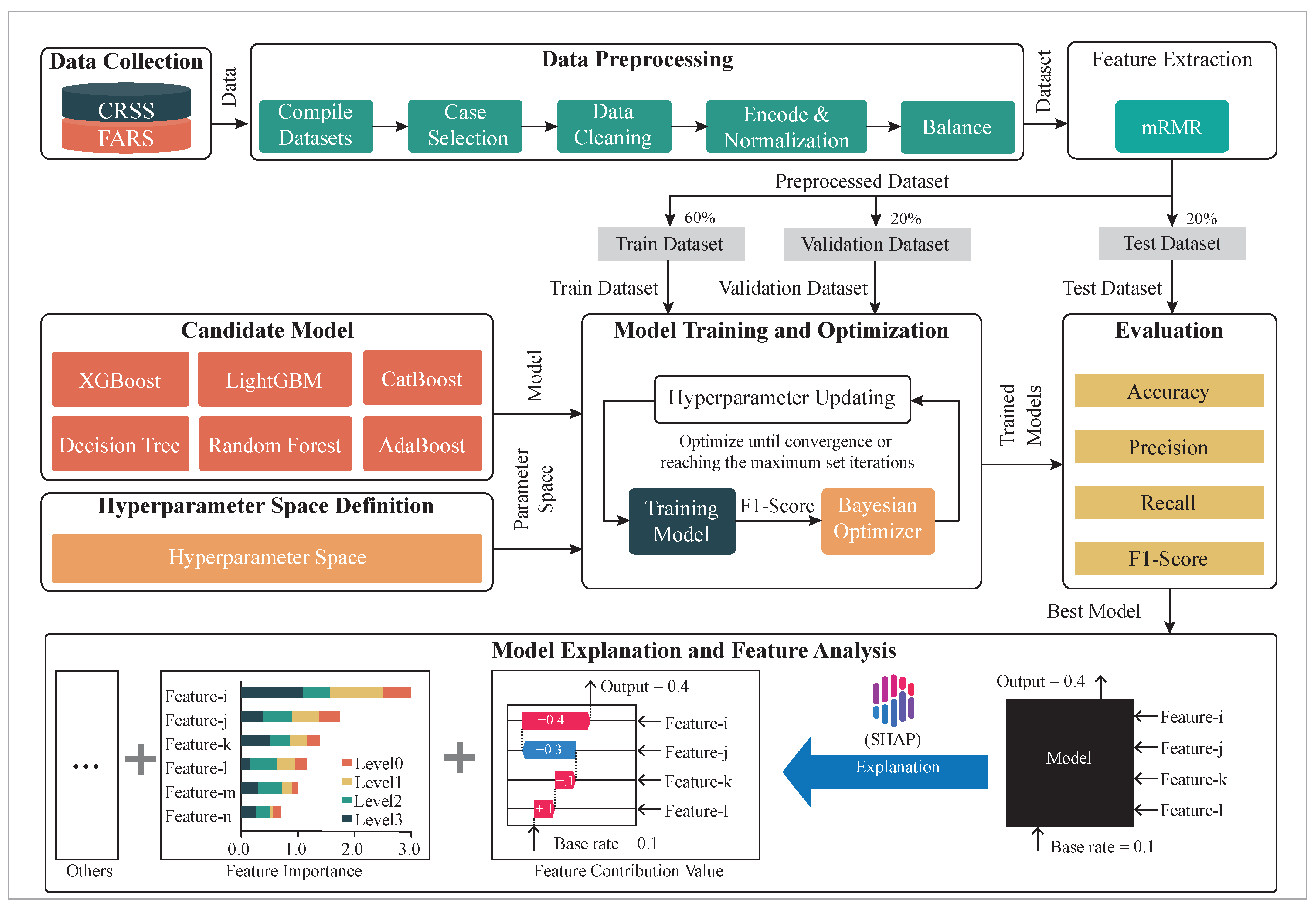
2. Methods
2.1. Accident Data Collection and Preprocessing
2.1.1. Accident Data Collection
2.1.2. Dataset Preprocessing
Dataset Compilation
Case Selection
Data Cleaning
Encoding and Normalization
Data Balancing
2.2. Feature Selection
2.2.1. Mutual Information (MI) Definition
2.2.2. Maximum Relevance Criterion
2.2.3. Minimum Redundancy Criterion
2.2.4. mRMR Optimization Objective
2.3. Prediction Model
2.3.1. Decision Tree
2.3.2. Random Forest
2.3.3. LightGBM
2.3.4. XGBoost
2.3.5. CatBoost
2.3.6. AdaBoost
2.4. Model Interpretation and Feature Analysis
2.4.1. Shapley Values
2.4.2. Additivity Property
2.4.3. Consistency
2.4.4. Efficiency for Tree Models (Tree SHAP)
3. Data Description
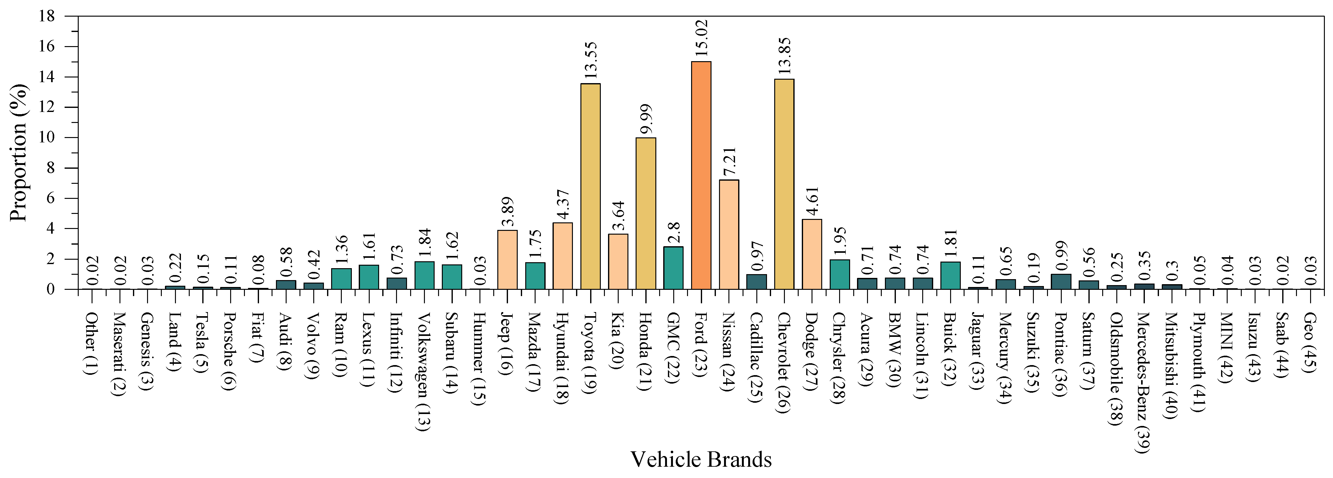
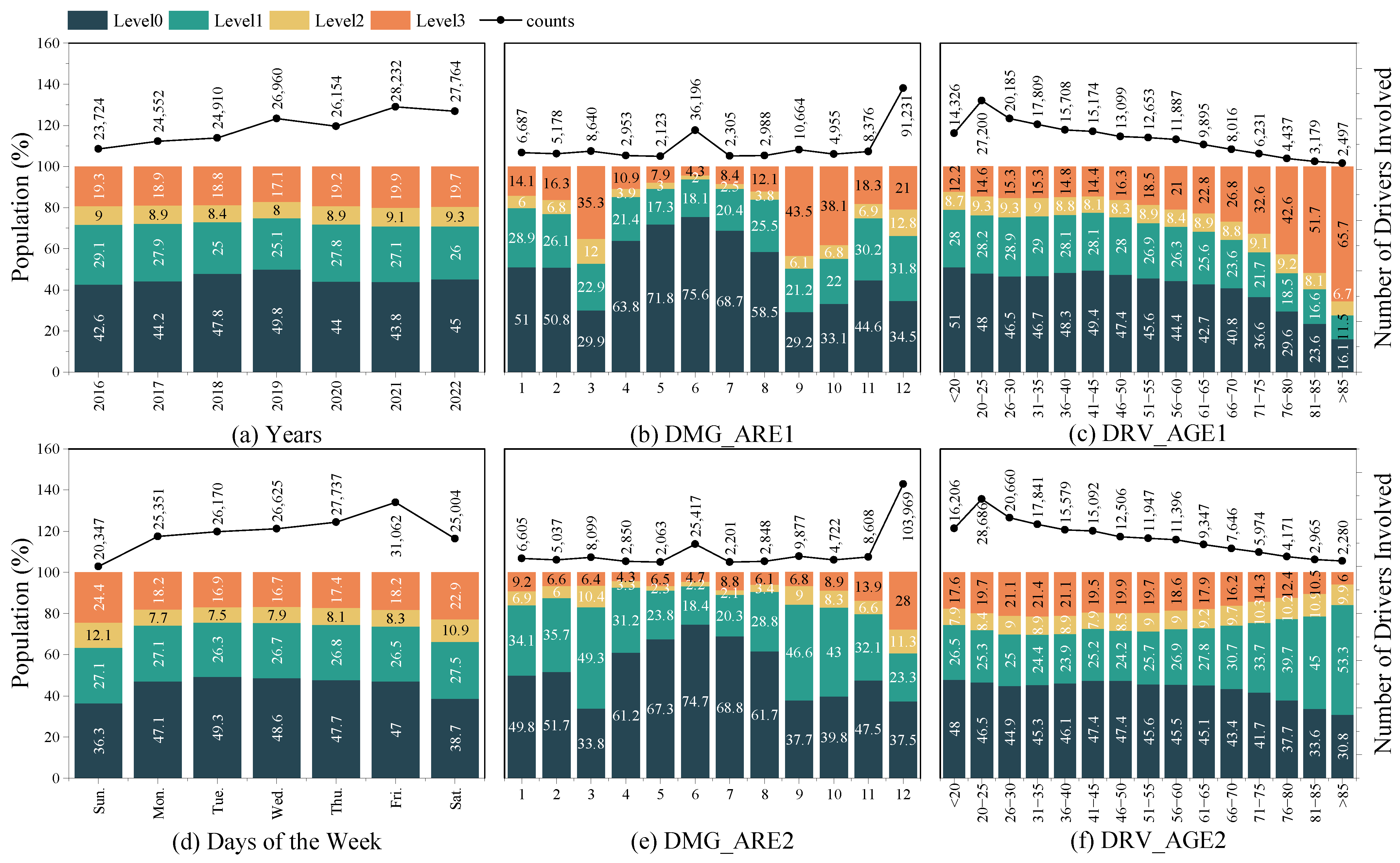
3.1. Descriptive Statistics of Accident Data
3.2. Feature Statistical Description
4. Experimental Results
4.1. Accident Feature Analysis
4.1.1. Feature Importance Analysis
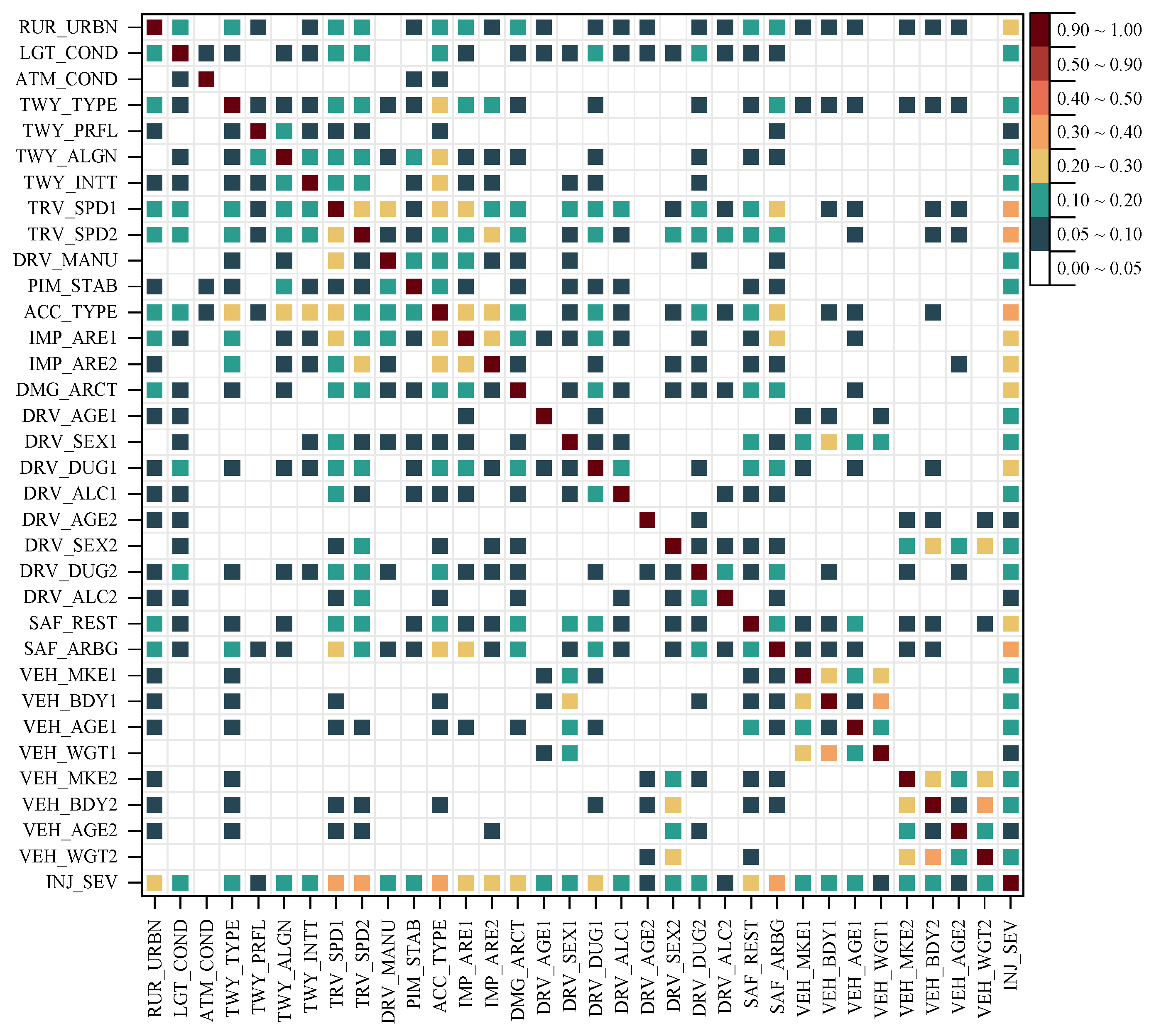
4.1.2. Feature Dependency Analysis
4.1.3. Bivariate SHAP Contribution Analysis
4.1.4. Instance-Level SHAP Interpretation
5. Implication and Limitations
5.1. Implications
5.2. Limitations
5.3. Future Work
6. Conclusions
Author Contributions
Funding
Institutional Review Board Statement
Informed Consent Statement
Data Availability Statement
Conflicts of Interest
Appendix A

References
- European Automobile Manufacturers’ Association (ACEA). ACEA Pocket Guide 2024–2025; Report No. N/A; European Automobile Manufacturers’ Association: Brussels, Belgium, 2024. [Google Scholar]
- International Transport Forum (ITF). Road Safety Annual Report 2024; OECD Publishing: Paris, France, 2024. [Google Scholar]
- Guo, W.; Li, J.; Song, X.; Zhang, W. A game-theoretic driver steering model with individual risk perception field generation. Accid. Anal. Prev. 2025, 211, 107869. [Google Scholar] [CrossRef]
- International Organization for Standardization. Road Vehicles–Types–Terms and Definitions (ISO Standard No. 3833:1977). 1977. Available online: https://www.iso.org/standard/9389.html (accessed on 25 December 2024).
- World Health Organization. Global Status Report on Road Safety 2023; World Health Organization: Geneva, Switzerland, 2023.
- National Center for Statistics and Analysis. Traffic Safety Facts 2022: A Compilation of Motor Vehicle Traffic Crash Data; Report No. DOT HS 813 656; National Highway Traffic Safety Administration: Washington, DC, USA, 2024.
- Guo, W.; Song, X.; Zhang, W.; Li, J.; Wu, X. Game-Theoretic Shared Control Strategy for Cooperative Collision Avoidance Under Extreme Conditions. IEEE Trans. Veh. Technol. 2024, 74, 246–262. [Google Scholar] [CrossRef]
- Chand, A.; Jayesh, S.; Bhasi, A.B. Road traffic accidents: An overview of data sources, analysis techniques and contributing factors. Mater. Today Proc. 2021, 47, 5135–5141. [Google Scholar] [CrossRef]
- Pourroostaei Ardakani, S.; Liang, X.; Mengistu, K.T.; So, R.S.; Wei, X.; He, B.; Cheshmehzangi, A. Road car accident prediction using a machine-learning-enabled data analysis. Sustainability 2023, 15, 5939. [Google Scholar] [CrossRef]
- Setiadi, D.R.I.M.; Islam, H.M.M.; Trisnapradika, G.A.; Herowati, W. Analyzing preprocessing impact on machine learning classifiers for cryotherapy and immunotherapy dataset. J. Future Artif. Intell. Technol. 2024, 1, 39–50. [Google Scholar] [CrossRef]
- Song, D.; Yang, X.; Yang, Y.; Cui, P.; Zhu, G. Bivariate joint analysis of injury severity of drivers in truck-car crashes accommodating multilayer unobserved heterogeneity. Accid. Anal. Prev. 2023, 190, 107175. [Google Scholar] [CrossRef]
- Gong, H.; Fu, T.; Sun, Y.; Guo, Z.; Cong, L.; Hu, W.; Ling, Z. Two-vehicle driver-injury severity: A multivariate random parameters logit approach. Anal. Methods Accid. Res. 2022, 33, 100190. [Google Scholar] [CrossRef]
- Cerwick, D.M.; Gkritza, K.; Shaheed, M.S.; Hans, Z. A comparison of the mixed logit and latent class methods for crash severity analysis. Anal. Methods Accid. Res. 2014, 3, 11–27. [Google Scholar] [CrossRef]
- Sheikh, M.S.; Peng, Y. Modeling collision risk for unsafe lane-changing behavior: A lane-changing risk index approach. Alex. Eng. J. 2024, 88, 164–181. [Google Scholar] [CrossRef]
- Zhang, J.; Jin, M.; Wan, C.; Dong, Z.; Wu, X. A Bayesian network-based model for risk modeling and scenario deduction of collision accidents of inland intelligent ships. Reliab. Eng. Syst. Saf. 2024, 243, 109816. [Google Scholar] [CrossRef]
- Liu, Z.; Chen, Y.; Xia, F.; Bian, J.; Zhu, B.; Shen, G.; Kong, X. TAP: Traffic Accident Profiling via Multi-Task Spatio-Temporal Graph Representation Learning. ACM Trans. Knowl. Discov. Data 2023, 17, 1–25. [Google Scholar] [CrossRef]
- Santos, K.; Dias, J.P.; Amado, C. A literature review of machine learning algorithms for crash injury severity prediction. J. Saf. Res. 2022, 80, 254–269. [Google Scholar] [CrossRef]
- Shaik, M.E.; Islam, M.M.; Hossain, Q.S. A review on neural network techniques for the prediction of road traffic accident severity. Asian Transp. Stud. 2021, 7, 100040. [Google Scholar] [CrossRef]
- Yu, L.; Du, B.; Hu, X.; Sun, L.; Han, L.; Lv, W. Deep spatio-temporal graph convolutional network for traffic accident prediction. Neurocomputing 2021, 423, 135–147. [Google Scholar] [CrossRef]
- Alhaek, F.; Liang, W.; Rajeh, T.M.; Javed, M.H.; Li, T. Learning spatial patterns and temporal dependencies for traffic accident severity prediction: A deep learning approach. Knowl.-Based Syst. 2024, 286, 111406. [Google Scholar] [CrossRef]
- Jamal, A.; Zahid, M.; Tauhidur Rahman, M.; Al-Ahmadi, H.M.; Almoshaogeh, M.; Farooq, D.; Ahmad, M. Injury severity prediction of traffic crashes with ensemble machine learning techniques: A comparative study. Int. J. Inj. Control Saf. Promot. 2021, 28, 408–427. [Google Scholar] [CrossRef]
- Yan, M.; Shen, Y. Traffic accident severity prediction based on random forest. Sustainability 2022, 14, 1729. [Google Scholar] [CrossRef]
- Wu, S.; Yuan, Q.; Yan, Z.; Xu, Q. Analyzing accident injury severity via an extreme gradient boosting (XGBoost) model. J. Adv. Transp. 2021, 2021, 3771640. [Google Scholar] [CrossRef]
- Otchere, D.A.; Ganat, T.O.A.; Ojero, J.O.; Tackie-Otoo, B.N.; Taki, M.Y. Application of gradient boosting regression model for the evaluation of feature selection techniques in improving reservoir characterisation predictions. J. Pet. Sci. Eng. 2022, 208, 109244. [Google Scholar] [CrossRef]
- Guo, M.; Yuan, Z.; Janson, B.; Peng, Y.; Yang, Y.; Wang, W. Older pedestrian traffic crashes severity analysis based on an emerging machine learning XGBoost. Sustainability 2021, 13, 926. [Google Scholar] [CrossRef]
- Dong, S.; Khattak, A.; Ullah, I.; Zhou, J.; Hussain, A. Predicting and analyzing road traffic injury severity using boosting-based ensemble learning models with SHAPley Additive exPlanations. Int. J. Environ. Res. Public Health 2022, 19, 2925. [Google Scholar] [CrossRef]
- Zahid, M.; Habib, M.F.; Ijaz, M.; Ameer, I.; Ullah, I.; Ahmed, T.; He, Z. Factors affecting injury severity in motorcycle crashes: Different age groups analysis using CatBoost and SHAP techniques. Traffic Inj. Prev. 2024, 25, 472–481. [Google Scholar] [CrossRef] [PubMed]
- Ahmed, S.; Hossain, M.A.; Bhuiyan, M.M.I.; Ray, S.K. A comparative study of machine learning algorithms to predict road accident severity. In Proceedings of the 2021 20th International Conference on Ubiquitous Computing and Communications (IUCC/CIT/DSCI/SmartCNS), London, UK, 20–22 December 2021; pp. 390–397. [Google Scholar]
- Wen, X.; Xie, Y.; Jiang, L.; Li, Y.; Ge, T. On the interpretability of machine learning methods in crash frequency modeling and crash modification factor development. Accid. Anal. Prev. 2022, 168, 106617. [Google Scholar] [CrossRef] [PubMed]
- Lundberg, S.M.; Erion, G.; Chen, H.; DeGrave, A.; Prutkin, J.M.; Nair, B.; Katz, R.; Himmelfarb, J.; Bansal, N.; Lee, S. From local explanations to global understanding with explainable AI for trees. Nat. Mach. Intell. 2020, 2, 56–67. [Google Scholar] [CrossRef] [PubMed]
- Ahmed, S.; Hossain, M.A.; Ray, S.K.; Bhuiyan, M.M.I.; Sabuj, S.R. A study on road accident prediction and contributing factors using explainable machine learning models: Analysis and performance. Transp. Res. Interdiscip. Perspect. 2023, 19, 100814. [Google Scholar] [CrossRef]
- Boo, Y.; Choi, Y. Comparison of mortality prediction models for road traffic accidents: An ensemble technique for imbalanced data. BMC Public Health 2022, 22, 1476. [Google Scholar] [CrossRef]
- Wongvorachan, T.; He, S.; Bulut, O. A comparison of undersampling, oversampling, and SMOTE methods for dealing with imbalanced classification in educational data mining. Information 2023, 14, 54. [Google Scholar] [CrossRef]
- Peng, H.; Long, F.; Ding, C. Feature selection based on mutual information criteria of max-dependency, max-relevance, and min-redundancy. IEEE Trans. Pattern Anal. Mach. Intell. 2005, 27, 1226–1238. [Google Scholar] [CrossRef]
- Toğaçar, M.; Ergen, B.; Çömert, Z.; Özyurt, F. A deep feature learning model for pneumonia detection applying a combination of mRMR feature selection and machine learning models. IRBM 2020, 41, 212–222. [Google Scholar] [CrossRef]
- Ravikiran, H.K.; Deepak, R.; Deepak, H.A.; Prapulla Kumar, M.S.; Sharath, S.; Yogeesh, G.H. A robust framework for Alzheimer’s disease detection and staging: Incorporating multi-feature integration, MRMR feature selection, and Random Forest classification. Multimed. Tools Appl. 2024. [Google Scholar] [CrossRef]
- Wang, G.; Lauri, F.; Hassani, A.H.E. Feature selection by mRMR method for heart disease diagnosis. IEEE Access 2022, 10, 100786–100796. [Google Scholar] [CrossRef]
- Rezvani, S.; Wang, X. A broad review on class imbalance learning techniques. Appl. Soft Comput. 2023, 143, 110415. [Google Scholar]
- Kingsford, C.; Salzberg, S.L. What are decision trees? Nat. Biotechnol. 2008, 26, 1011–1013. [Google Scholar] [CrossRef]
- Breiman, L. Random forests. Mach. Learn. 2001, 45, 5–32. [Google Scholar] [CrossRef]
- Ke, G.; Meng, Q.; Finley, T.; Wang, T.; Chen, W.; Ma, W.; Ye, Q.; Liu, T.-Y. LightGBM: A highly efficient gradient boosting decision tree. Adv. Neural Inf. Process. Syst. 2017, 30, 3149–3157. [Google Scholar]
- Chen, T.; Guestrin, C. XGBoost: A Scalable Tree Boosting System. arXiv 2016, arXiv:1603.02754. Available online: https://arxiv.org/abs/1603.02754 (accessed on 20 December 2024).
- Prokhorenkova, L.; Gusev, G.; Vorobev, A.; Dorogush, A.V.; Gulin, A. CatBoost: Unbiased boosting with categorical features. Adv. Neural Inf. Process. Syst. 2018, 31, 6639–6649. [Google Scholar]
- Freund, Y.; Schapire, R.E. A decision-theoretic generalization of on-line learning and an application to boosting. J. Comput. Syst. Sci. 1997, 55, 119–139. [Google Scholar]
- Agresti, A. Categorical Data Analysis; John Wiley & Sons: Hoboken, NJ, USA, 2013. [Google Scholar]


| Database | Participants | Case Number | Driver Numbers for Different Accident Vehicles | ||||||
|---|---|---|---|---|---|---|---|---|---|
| Total | PV-PV | Total | PV | Motorcycle | Truck | Bus | Others | ||
| 1 | 121,288 | - | 121,288 | 107,169 | 8585 | 3768 | 418 | 1348 | |
| CRSS | 2 | 204,916 | 175,910 | 409,832 | 379,053 | 9341 | 14,218 | 1590 | 5630 |
| >2 | 26,938 | - | 87,755 | 83,664 | 883 | 2226 | 122 | 860 | |
| 1 | 134,982 | - | 134,982 | 111,851 | 14,360 | 5462 | 370 | 2939 | |
| FARS | 2 | 86,718 | 49,551 | 173,436 | 132,888 | 18,678 | 17,512 | 580 | 3778 |
| >2 | 19,931 | - | 69,080 | 57,565 | 3685 | 6361 | 177 | 1292 | |
| CRSS + FARS | - | 594,773 | 225,461 | 996,373 | 872,190 | 55,532 | 49,547 | 3257 | 15,847 |
| Variables | (%) | Injury Severity (%) | Variables | (%) | Injury Severity (%) | ||||||
|---|---|---|---|---|---|---|---|---|---|---|---|
| 0 | 1 | 2 | 3 | 0 | 1 | 2 | 3 | ||||
| Database | Divided, Unprotected (2) | 27.7 | 50.2 | 31.2 | 6.6 | 12 | |||||
| CRSS | 63.3 | 68.7 | 27.7 | 3.2 | 0.4 | Divided, Protected (3) | 13.4 | 58 | 22.8 | 5.6 | 13.6 |
| FARS | 36.7 | 5 | 25.5 | 18.4 | 51.1 | One-Way (4) | 7.4 | 72.5 | 19.9 | 3.1 | 4.6 |
| CRSS + FARS | 100 | 45.3 | 26.9 | 8.8 | 19 | Roadway Profile (TWY_PRFL) | |||||
| Location at rural or urban (RUR_URBN) | Level (1) | 85.9 | 47.5 | 26.9 | 8.1 | 17.5 | |||||
| Rural (1) | 67.9 | 53 | 25.6 | 7.7 | 13.7 | Grade (2) | 7.2 | 36.1 | 27.7 | 11.4 | 24.8 |
| Urban (2) | 32.1 | 29.1 | 29.5 | 11.3 | 30.2 | Uphill (3) | 2.4 | 28.8 | 25.7 | 15 | 30.5 |
| Light condition (LGT_COND) | Downhill (4) | 2.7 | 31.2 | 24.5 | 13.6 | 30.7 | |||||
| Daylight (1) | 69.8 | 50.6 | 26.8 | 7.2 | 15.4 | Hillcrest (5) | 1.5 | 23.2 | 27.3 | 15.2 | 34.3 |
| Dawn (2) | 1.6 | 34 | 25 | 12 | 29.1 | Sag (6) | 0.2 | 26.6 | 31.2 | 11.6 | 30.7 |
| Dusk (3) | 2.6 | 47.6 | 24.8 | 9.3 | 18.3 | Roadway Alignment (TWY_ALGN) | |||||
| Dark-Lighted (4) | 15 | 41.1 | 30.5 | 9.4 | 19 | Straight (1) | 91.6 | 47.2 | 27.4 | 8.1 | 17.4 |
| Dark-Not Lighted (5) | 11 | 19.2 | 22.9 | 17.5 | 40.4 | Curve Right (2) | 4.6 | 31.1 | 19.1 | 14.9 | 35 |
| Atmospheric Conditions (ATM_COND) | Curve Left (3) | 3.8 | 18 | 24 | 19.5 | 38.5 | |||||
| Clear (1) | 74.4 | 46.3 | 26.6 | 8.6 | 18.5 | Type of Intersection (TWY_INTT) | |||||
| Cloudy (2) | 14.8 | 43.1 | 27.6 | 9.3 | 20.1 | Four-Way Intersection (1) | 33.7 | 45.9 | 33.3 | 6.8 | 14 |
| Rain (3) | 8.6 | 44.5 | 27.6 | 8.6 | 19.2 | T-Intersection (2) | 14.4 | 46.2 | 34.1 | 6.2 | 13.5 |
| Snow (4) | 1.2 | 41.3 | 26.8 | 11.1 | 20.9 | Roundabout (3) | 0.2 | 84.4 | 13.4 | 0.6 | 1.6 |
| Fog (5) | 0.6 | 17.7 | 24.6 | 17.6 | 40.1 | Five-Point, or more (4) | 0.2 | 55.5 | 29.7 | 5.9 | 8.9 |
| Other (6) | 0.3 | 22 | 26.4 | 17.3 | 34.4 | Y-Intersection (5) | 0 | 47.2 | 33.3 | 2.8 | 16.7 |
| Trafficway Description (TWY_TYPE) | Other Type (6) | 0.4 | 29.8 | 29.8 | 11.3 | 29.1 | |||||
| Not Divided (1) | 51.5 | 35.6 | 26.6 | 11.6 | 26.2 | Non-intersection (7) | 51.1 | 44.7 | 20.6 | 10.9 | 23.9 |
| Variables | (%) | Injury Severity (%) | Variables | (%) | Injury Severity (%) | ||||||
|---|---|---|---|---|---|---|---|---|---|---|---|
| 0 | 1 | 2 | 3 | 0 | 1 | 2 | 3 | ||||
| Attempted Avoidance Maneuver (DRV_MANU) | Intersect Paths (Straight Path) (7) | 14.3 | 26.1 | 40.6 | 9.9 | 23.5 | |||||
| No Avoidance Maneuver (1) | 23.7 | 62.6 | 17.6 | 5.7 | 14.2 | Opposite Direction (Angle Sideswipe) (8) | 4.2 | 12.4 | 28.4 | 16.5 | 42.8 |
| Braking (2) | 3.5 | 51.6 | 32.8 | 7.5 | 8.2 | Head-On (9) | 14.7 | 2.2 | 16.1 | 27.1 | 54.6 |
| Unknown (3) | 68 | 40.7 | 29.5 | 9.3 | 20.5 | Other Types (10) | 0.3 | 8.2 | 23.4 | 10.9 | 57.5 |
| Accelerating (4) | 0.1 | 39.5 | 29.3 | 10.9 | 20.4 | Travel Speed of This Vehicle (TRV_SPD1) | |||||
| Braking and Steering (5) | 1 | 24.7 | 35.9 | 18.3 | 21 | 0 mph | 16.2 | 84.6 | 11.3 | 1.4 | 2.7 |
| Releasing Brakes (6) | 0 | 22.9 | 41.7 | 2.1 | 33.3 | 0–20 mph | 19 | 82.2 | 8.8 | 2.2 | 6.8 |
| Braking and Unknown Steering Direction (7) | 0.2 | 13.4 | 42.9 | 18.8 | 25 | 21–40 mph | 27.1 | 38.1 | 41.5 | 7.2 | 13.2 |
| Steering (8) | 3.5 | 20.9 | 28.6 | 19 | 31.5 | 41–60 mph | 28.2 | 15.5 | 34.2 | 16.2 | 34.1 |
| Accelerating and Steering (9) | 0 | 26.1 | 19.5 | 16.3 | 38.2 | >60 mph | 9.4 | 13.7 | 25.9 | 17.4 | 43.1 |
| Pre-Impact Stability (PIM_STAB) | Travel Speed of Other Vehicle (TRV_SPD2) | ||||||||||
| Tracking (1) | 92.6 | 48 | 27.1 | 8.2 | 16.7 | 0 mph | 10 | 73 | 21.2 | 2.4 | 3.4 |
| Skidding Longitudinally (2) | 1.4 | 26.5 | 31.1 | 14.5 | 27.9 | 0–20 mph | 18.9 | 79.3 | 15.9 | 2.4 | 2.3 |
| Skidding Laterally (3) | 1.1 | 5.6 | 8.5 | 14.9 | 70.9 | 21–40 mph | 30 | 46.8 | 35.8 | 6.4 | 11 |
| Other (4) | 4.9 | 10.2 | 24.9 | 17.2 | 47.7 | 41–60 mph | 30.9 | 23.1 | 28.4 | 14.7 | 33.8 |
| Crash Type (ACC_TYPE) | >60 mph | 10.1 | 18.2 | 21.4 | 16.2 | 44.2 | |||||
| Rear End (1) | 32.1 | 74.9 | 18.6 | 2.1 | 4.4 | Damage Area Count (DMG_ARCT) | |||||
| Same Direction (Angle, Sideswipe) (2) | 7 | 79 | 11 | 1.8 | 8.2 | 1 | 55.9 | 52.9 | 26.1 | 6.9 | 14 |
| Miss Control (3) | 1.2 | 90.1 | 6.5 | 1.1 | 2.4 | 2–5 | 35.2 | 44.1 | 30.9 | 8.4 | 16.6 |
| Turn Into Path (4) | 12.2 | 42.1 | 37.2 | 5.9 | 14.8 | 6–9 | 4.7 | 4.7 | 20.1 | 22.2 | 53 |
| Turn Across Path (5) | 13.5 | 36 | 43.8 | 7.9 | 12.2 | 10–12 | 4.2 | 1.1 | 10.4 | 21.9 | 66.6 |
| Opposite direction (Forward Impact) (6) | 0.4 | 1.7 | 34.7 | 21.9 | 41.7 | ||||||
| Variables | (%) | Injury Severity (%) | Variables | (%) | Injury Severity (%) | ||||||
|---|---|---|---|---|---|---|---|---|---|---|---|
| 0 | 1 | 2 | 3 | 0 | 1 | 2 | 3 | ||||
| The gender of this driver (DRV_SEX1) | <1 | 4.7 | 54.8 | 21.5 | 6.5 | 17.2 | |||||
| Male (1) | 55.9 | 44.7 | 23.7 | 9.5 | 22 | 1–10 | 55.9 | 49.3 | 24.7 | 7.6 | 18.4 |
| Female (2) | 44.1 | 46.2 | 30.8 | 7.9 | 15.2 | 11–20 | 34.1 | 39.6 | 29.8 | 10.5 | 20.1 |
| Drug involvement of this driver (DRV_DUG1) | >20 | 5.3 | 32.4 | 35.3 | 12.7 | 19.7 | |||||
| No (1) | 96.6 | 46.8 | 27.2 | 8.3 | 17.7 | The Weight of This Vehicle (VEH_WGT1) | |||||
| Yes (2) | 3.4 | 3.9 | 17.1 | 22.5 | 56.6 | 1700–2700 lbs. | 8.5 | 38.2 | 21.3 | 8.2 | 32.5 |
| Alcohol Test Result of this driver (DRV_ALC1) | 2701–3700 lbs. | 51.9 | 44.8 | 25.9 | 8.4 | 21 | |||||
| 0 mg/dL | 93.7 | 48 | 27.4 | 8.2 | 16.5 | 3701–4700 lbs. | 26.3 | 48.3 | 28.3 | 9.2 | 14.2 |
| 1–80 mg/dL | 1 | 2.7 | 14.8 | 15.9 | 66.5 | 4701–5700 lbs. | 11.2 | 47.4 | 30.6 | 10.1 | 11.9 |
| >80 mg/dL | 5.4 | 7.7 | 18.7 | 19 | 54.6 | >5700 lbs. | 2.1 | 40.7 | 34.6 | 10.9 | 13.9 |
| The Other Driver’s Gende (DRV_SEX2) | The Weight of Other Vehicle (VEH_WGT2) | ||||||||||
| Male (1) | 58 | 41 | 26.6 | 9.8 | 22.7 | 1700–2700 lbs. | 8 | 47.77 | 35.4 | 9.45 | 7.38 |
| Female (2) | 42 | 51.4 | 27.2 | 7.5 | 13.9 | 2701–3700 lbs. | 50.1 | 48.77 | 28.8 | 8.91 | 13.52 |
| Drug Involvement of Other Driver (DRV_DUG2) | 3701–4700 lbs. | 27 | 44.53 | 24.96 | 8.47 | 22.04 | |||||
| No (1) | 96.6 | 46.7 | 26.9 | 8.3 | 18.2 | 4701–5700 lbs. | 12.4 | 35.65 | 19.91 | 8.51 | 35.93 |
| Yes (2) | 3.4 | 7.8 | 25.9 | 22.9 | 43.5 | >5700 lbs. | 2.5 | 25.54 | 14.95 | 9.9 | 49.61 |
| Alcohol Test Result of other driver (DRV_ALC2) | Vehicle Body Type of This Vehicle (VEH_BDY1) | ||||||||||
| 0 mg/dL | 93.7 | 47.7 | 26.8 | 8 | 17.6 | Pickup (1) | 15.7 | 45 | 27.7 | 10.4 | 16.9 |
| 1–80 mg/dL | 0.9 | 6.6 | 29 | 23 | 42 | SUV (2) | 30 | 50.2 | 28.7 | 8.4 | 12.7 |
| >80 mg/dL | 5.4 | 11.6 | 27.2 | 21.2 | 40.1 | Minivan (3) | 2.1 | 69.1 | 27.8 | 2.8 | 0.3 |
| Seat Belt Type and Usage Status (SAF_REST) | Cargo Van (4) | 0.3 | 80.8 | 17.5 | 1.5 | 0.2 | |||||
| Not Used (1) | 12.7 | 9.9 | 14.8 | 16.9 | 58.4 | VAN (5) | 1.9 | 11 | 30.2 | 18.8 | 40 |
| Two–Point (2) | 0.9 | 41.3 | 35.2 | 8.4 | 15.1 | Sedan (6) | 40.7 | 43.2 | 25.8 | 8.5 | 22.5 |
| Three–Point (3) | 84.7 | 50.9 | 28.4 | 7.5 | 13.2 | Coupe (7) | 3.7 | 38.6 | 22.9 | 9.4 | 29.1 |
| Others (4) | 1.7 | 34 | 33 | 16 | 17 | Wagon (8) | 0.7 | 41.8 | 23 | 6.6 | 28.7 |
| Air bag deployment (SAF_ARBG) | Hatchback (9) | 4.1 | 41.1 | 24.4 | 7.9 | 26.6 | |||||
| Not Deployed (1) | 58 | 71.2 | 17.8 | 3 | 8.1 | Convertible (10) | 0.8 | 39.1 | 21.8 | 8.5 | 30.6 |
| Curtain (2) | 0.1 | 10.2 | 30.5 | 15.3 | 44.1 | Vehicle Body Type of Other Vehicle (VEH_BDY2) | |||||
| Side (3) | 1.2 | 19 | 39 | 8.2 | 34 | Pickup (1) | 17.3 | 34.9 | 20.8 | 9.2 | 35.1 |
| Front (4) | 1.2 | 18.8 | 38.7 | 8.2 | 34.4 | SUV (2) | 29.8 | 48.2 | 25 | 7.8 | 19 |
| Combined (5) | 16 | 10.1 | 39 | 16.7 | 34.2 | Minivan (3) | 2.1 | 67.1 | 28.9 | 3.6 | 0.4 |
| Other (6) | 24.4 | 8.7 | 39.8 | 17.4 | 34 | Cargo Van (4) | 0.4 | 68.3 | 27.6 | 3.9 | 0.2 |
| The Age of This Vehicle (VEH_AGE1) | VAN (5) | 2 | 9.2 | 23 | 18 | 49.8 | |||||
| <1 | 5 | 53.7 | 30.3 | 6.9 | 9.1 | Sedan (6) | 39.5 | 48.3 | 29.9 | 9.1 | 12.8 |
| 1–10 | 56.8 | 49.7 | 29.3 | 7.8 | 13.1 | Coupe (7) | 3.6 | 42.1 | 31.4 | 10.5 | 16 |
| 11–20 | 32.7 | 39.5 | 23.6 | 10.4 | 26.6 | Wagon (8) | 0.7 | 46.1 | 31.7 | 10 | 12.2 |
| >20 | 5.4 | 26.7 | 17.3 | 12.1 | 43.9 | Hatchback (9) | 3.8 | 48.8 | 30.9 | 8.6 | 11.7 |
| The Age of Other Vehicle (VEH_AGE2) | Convertible (10) | 0.8 | 41.9 | 34.3 | 10.3 | 13.6 | |||||
| Models | Injury Severity | Imbalanced Data (%) | Balanced Data (%) | ||||||
|---|---|---|---|---|---|---|---|---|---|
| Precision | Recall | F1-Score | Accuracy | Precision | Recall | F1-Score | Accuracy | ||
| Level 0 | 87.93 | 90.81 | 89.34 | 85.19 | 87.19 | 86.17 | |||
| Level 1 | 72.17 | 74.02 | 73.08 | 79.12 | 76.99 | 78.04 | |||
| XGBoost | Level 2 | 51.55 | 20.95 | 29.79 | 86.66 | 85.88 | 86.27 | ||
| Level 3 | 75.57 | 88.07 | 81.34 | 88.42 | 89.55 | 88.98 | |||
| Average | 71.80 | 68.46 | 68.39 | 79.52 | 84.85 | 84.90 | 84.87 | 84.90 | |
| Level 0 | 87.85 | 90.07 | 88.95 | 84.69 | 86.85 | 85.76 | |||
| Level 1 | 71.01 | 74.28 | 72.61 | 79.74 | 74.47 | 77.01 | |||
| Random | Leve l2 | 54.96 | 15.33 | 23.97 | 86.00 | 87.88 | 86.93 | ||
| Forest | Level 3 | 72.74 | 88.33 | 79.78 | 88.11 | 89.75 | 88.92 | ||
| Average | 71.64 | 67.01 | 66.33 | 78.81 | 84.63 | 84.74 | 84.66 | 83.74 | |
| Level 0 | 88.16 | 90.20 | 89.17 | 84.38 | 86.43 | 85.39 | |||
| Level 1 | 71.60 | 74.19 | 72.87 | 75.83 | 75.05 | 75.44 | |||
| CatBoost | Level 2 | 49.39 | 23.59 | 31.93 | 81.07 | 79.31 | 80.18 | ||
| Level 3 | 75.82 | 86.42 | 80.77 | 84.68 | 85.38 | 85.03 | |||
| Average | 71.24 | 68.60 | 68.69 | 79.22 | 81.49 | 81.54 | 81.51 | 81.52 | |
| Level 0 | 87.88 | 90.28 | 89.06 | 83.87 | 86.03 | 84.93 | |||
| Level 1 | 71.18 | 72.30 | 71.74 | 73.84 | 74.27 | 74.06 | |||
| LightGBM | Level 2 | 42.18 | 24.21 | 30.76 | 77.72 | 73.80 | 75.71 | ||
| Level 3 | 75.32 | 83.86 | 79.36 | 81.04 | 82.67 | 81.85 | |||
| Average | 69.14 | 67.66 | 67.73 | 78.31 | 79.12 | 79.19 | 79.14 | 79.15 | |
| Level 0 | 88.81 | 84.61 | 86.66 | 85.03 | 77.86 | 81.29 | |||
| Level 1 | 63.38 | 77.87 | 69.88 | 69.39 | 78.04 | 73.46 | |||
| AdaBoost | Level 2 | 51.16 | 20.92 | 29.70 | 80.52 | 74.09 | 77.17 | ||
| Level 3 | 77.01 | 82.07 | 79.46 | 80.65 | 83.89 | 82.24 | |||
| Average | 70.09 | 66.37 | 66.43 | 76.62 | 78.90 | 78.47 | 78.54 | 78.45 | |
| Level 0 | 84.50 | 86.85 | 85.66 | 80.26 | 81.56 | 80.91 | |||
| Level 1 | 63.95 | 63.95 | 63.95 | 64.50 | 65.64 | 65.07 | |||
| Decision | Level 2 | 37.56 | 24.15 | 29.40 | 65.36 | 66.99 | 66.17 | ||
| Tree | Level 3 | 69.71 | 70.59 | 70.15 | 75.53 | 71.07 | 73.23 | ||
| Average | 63.93 | 61.39 | 62.29 | 72.00 | 71.42 | 71.32 | 71.34 | 71.27 | |
Disclaimer/Publisher’s Note: The statements, opinions and data contained in all publications are solely those of the individual author(s) and contributor(s) and not of MDPI and/or the editor(s). MDPI and/or the editor(s) disclaim responsibility for any injury to people or property resulting from any ideas, methods, instructions or products referred to in the content. |
© 2025 by the authors. Licensee MDPI, Basel, Switzerland. This article is an open access article distributed under the terms and conditions of the Creative Commons Attribution (CC BY) license (https://creativecommons.org/licenses/by/4.0/).
Share and Cite
Liu, P.; Zhang, W.; Wu, X.; Guo, W.; Yu, W. Driver Injury Prediction and Factor Analysis in Passenger Vehicle-to-Passenger Vehicle Collision Accidents Using Explainable Machine Learning. Vehicles 2025, 7, 42. https://doi.org/10.3390/vehicles7020042
Liu P, Zhang W, Wu X, Guo W, Yu W. Driver Injury Prediction and Factor Analysis in Passenger Vehicle-to-Passenger Vehicle Collision Accidents Using Explainable Machine Learning. Vehicles. 2025; 7(2):42. https://doi.org/10.3390/vehicles7020042
Chicago/Turabian StyleLiu, Peng, Weiwei Zhang, Xuncheng Wu, Wenfeng Guo, and Wangpengfei Yu. 2025. "Driver Injury Prediction and Factor Analysis in Passenger Vehicle-to-Passenger Vehicle Collision Accidents Using Explainable Machine Learning" Vehicles 7, no. 2: 42. https://doi.org/10.3390/vehicles7020042
APA StyleLiu, P., Zhang, W., Wu, X., Guo, W., & Yu, W. (2025). Driver Injury Prediction and Factor Analysis in Passenger Vehicle-to-Passenger Vehicle Collision Accidents Using Explainable Machine Learning. Vehicles, 7(2), 42. https://doi.org/10.3390/vehicles7020042