Article

Integrated Sensing and New Radio Communications for Air Vehicle Positioning

by
Ibrahima Mbaye
,
Saba Al-Rubaye
*,
Christopher Conrad
and
Gokhan Inalhan
Centre for Autonomous and Cyberphysical Systems, Cranfield University, Bedfordshire MK43 0AL, UK
*
Author to whom correspondence should be addressed.
Vehicles 2024, 6(3), 1665-1689; https://doi.org/10.3390/vehicles6030080
Submission received: 29 July 2024 / Revised: 7 September 2024 / Accepted: 17 September 2024 / Published: 23 September 2024

Abstract

:
Aerial vehicles are increasingly relying on connectivity to cellular networks, with 5G new radio (NR) and 6G technologies deemed critical for the next generation of indoor and outdoor positioning systems. Conventional time of arrival approaches require time synchronisation between base stations and vehicles, and a clock bias greater than 30 ns can result in a positioning inaccuracy above 10 m. This work, thereby, proposes an integrated positioning technique based on RF fingerprinting using ray-tracing data and reinforced with machine learning. The system leverages advanced sensing technologies, NR communications, and AI-driven random forests to enhance the precision and reliability of air vehicle positioning, contributing to safer and more efficient air travel and autonomous flight operations. The developed solution is evaluated in a representative urban canyon environment, in which the performance of conventional radio-based positioning systems is often degraded. Notably, a supervised learning algorithm based on the received signal strength and time of arrival is shown to exhibit an accuracy of under 3 m in 75% of the areas studied.

1. Introduction

The use of cellular networks for vehicle connectivity is becoming increasingly popular due to recent developments in the telecommunications sector. Fifth-generation (5G) cellular networks are considered especially crucial for the next generation of indoor and outdoor positioning. This technology can offer unprecedented accuracy for applications requiring cm or dm level accuracy, including industrial automation, urban air mobility (UAM), and self-driving vehicles [1]. UAM is a revolutionary air transportation system for people and goods in urban areas. Electric aircraft take-off and land, either autonomously or with an onboard pilot, for applications such as “air-taxi”, drone delivery, and search and rescue. The strategic plans of several countries seek to gradually introduce UAM into formerly restricted airspace, including urban and suburban areas [2].
According to a survey carried out by the European Union Aviation Safety Agency (EASA) [3], the safety and security of UAM vehicles are among the top three concerns of citizens. In fact, 37% of the citizens who took the survey were concerned about the safety of “air-taxis” while 44% were concerned about the safety of other unmanned aircraft system (UAS) operations. Similarly, 44% and 37% of respondents expressed concern with the security of “air-taxis” and other UAS operations, respectively. Maintaining a level of safety equivalent to that of traditional aviation, therefore, remains a top priority, and UAM aircraft must satisfy performance-based navigation (PBN) standards for integrity, accuracy, continuity, and availability. Detect and avoid (DAA) systems especially rely on the performance of onboard navigation systems, confirming that a continuous and high-performance navigation system is necessary to implement a safe UAM infrastructure.
The availability of reliable positioning, navigation, and timing data is required for many intelligent transportation systems (ITSs). The advent of additional constellations such as GALILEO and GLONASS, together with that of multiconstellation receivers, has increased the service coverage and popularity of global navigation satellite systems (GNSSs) for vehicle location. This technology, however, offers a typical accuracy ranging from a few metres to over 25 m, limiting its use for unmanned vehicles where cm and dm level accuracy is required. A hybrid GNSS and inertial navigation system (INS) helps overcome standalone GNSS limitations for civilian UAS navigation systems. The INS contains gyroscopes and accelerometers for relative positioning estimates through dead-reckoning. Due to the buildup of measurement errors, however, INS performance degrades with time, and the drift-free positioning solution offered by GNSSs is often used to calibrate the INS sensors [4]. Nevertheless, GNSS performance is significantly degraded in dense urban areas, since it relies on an unrestricted line of sight (LOS) between the vehicle antenna and the orbiting satellites. Additionally, GNSS signals tend to suffer from atmospheric and relativistic effects, signal interference, and receiver noise [2].

Literature Gaps and Contributions

Positioning using 5G cellular networks has gained significant traction over the past decade. As the available bandwidth has increased for 5G new radio (NR), most research has focused on time-based methods, with the increased bandwidth lowering the theoretical lower bound for time of arrival (TOA) estimates [5]. Additionally, the high frequency carrier allows the use of smaller antennas for massive multiple input multiple output (MIMO) configurations, enabling the exploitation of angle of departure/arrival information to locate MIMO-enabled devices [6]. Combining GNSSs with mobile networks has also received much interest over the years [7,8,9], suggesting that cellular technologies can help address the limitations of GNSSs in urban areas.
Radio frequency (RF) fingerprinting involves extracting the hardware characteristics of a transmitter that are unintentionally embedded in its transmitted waveform [10]. The majority of research on RF fingerprinting, however, focuses on indoor positioning. While some research [11] has exploited RF fingerprinting techniques for mm-Wave signals, no evidence has been found on achieving sub-metre positioning accuracy using sub-6 GHz frequencies in outdoor urban areas. This work, thereby, studies the sub-6 GHz frequency spectrum in light of the current commercial deployment of 5G nonstandalone (NSA) and standalone (SA) modes in this band.
GNSS positioning is insufficiently precise and cost-effective for air vehicles operating in urban canyon environments. In many applications, positioning techniques based on cellular networks such as fourth-generation (4G) long-term evolution (LTE) have been used with GNSS to address its limitations. The 5G standalone positioning, however, also requires close synchronisation between base stations (BSs) and users and remains susceptible to multipath effects. The advent of 5G NR significantly improves the performance of positioning systems leveraging cellular networks [12]. Densification of the network reduces the likelihood of non-LOS (NLOS) propagation, and the availability of a wider bandwidth enhances the accuracy of TOA-based methods.
The authors in [13,14] illustrated the application of a machine learning (ML) classification algorithm based on random forest (RF) for addressing localisation challenges involving “noncollaborative” emitters in an outdoor environment, where the sensors lack prior knowledge of the signal. This technology merges the multipath fingerprint technique with ray-tracing (RT) simulations. The benefit of this approach is the ability to extract multipath fingerprints directly from received signals, bypassing the need for channel impulse response estimation.
This work, thereby, presents an artificial intelligence (AI)-driven methodology to enhance the precision and reliability of air vehicle positioning, using sub-6 GHz frequencies in outdoor urban areas. The main contributions of this work are as follows:
  • The literature on 5G NR positioning is reviewed and critically analysed.
  • A methodology to model the 5G environment in an urban canyon is proposed, using advanced ray-tracing simulations, capturing signal propagation characteristics such as reflections, scattering, and diffractions caused by buildings and obstacles.
  • An AI-driven RF fingerprinting technique is developed, leveraging received signal strength (RSS) and TOA data to improve positioning accuracy in multipath-rich environments.
  • Machine learning algorithms for positioning are designed and implemented, specifically using Bayesian regularized artificial neural networks (BRANNs) and random forests, to enhance the precision and robustness of positioning systems.
  • Random forests are shown to outperform BRANN-based models.
  • The proposed positioning system is extensively evaluated in a simulated urban canyon environment, demonstrating errors below 3 m in 75% of the areas studied.

2. Algorithm Development and Theory

This section introduces the theory underlying radio-positioning, multipath interference, and emerging 5G systems. It further describes AI and machine learning (ML) concepts that are fundamental to the algorithms developed in this paper.

2.1. Radio-Based Positioning

Waveforms are intrinsically tied to the geometry of their propagation environment, and the LOS components of a transmitted signal can be reflected, scattered, or diffracted by the obstacles in its surrounding. If these components do not interfere with each other, the LOS component is resolvable and provides an accurate measurement of the distance between transmitter and receiver. Notably, time-based, signal strength, and angle-based measurements may be used to estimate the user’s position. Each of these measurements has its own set of strengths and limitations, offering a trade-off between complexity, cost, and positioning accuracy:
  • Signal strength-based: The measurement of signal strength is related to the distance d between the receiver and transmitter through Equation (1):
    P r [ d B m ] = P 0 [ d B m ] + K [ d B m ] + 10 γ l o g 10 d d 0 ,
    where P 0 is the received power at a reference distance d 0 , K corresponds to the large-scale fading fluctuations often modelled as a Gaussian random variable with zero mean and standard deviation σ K , and  γ is the path loss exponent with a typical value between 2 and 6 [15]. The primary benefits of signal-strength-based methods are their low cost and the elimination of the need for node-to-node network time synchronisation. Nonetheless, the positioning accuracy achieved is typically low due to the complexity of signal strength fluctuations with distance, ranging from 10 m to 50 m. Notably, multipath fading causes frequency-selective fading that is random and unpredictable, and is particularly concerning for location systems in urban areas, where LOS is frequently obstructed [16].
  • Time-based: In time-based positioning, three approaches are typically used: one-way ranging TOA, two-way ranging round-trip time (RTT), and time difference of arrival (TDOA). When using TOA, measurements of the signal propagation delay, τ = d / c are used to obtain information about the separation distance between two nodes, where d is the distance between the nodes and c is the speed of the light. Using 2D geometry, a circle represents the receiver’s estimated range from each BS, and the intersections of circles represent the receiver location, as depicted in Figure 1. However, the intersection of these circles is often not an unique point due to measurement inaccuracies and multipath effects.
  • Angle-based: Angle-based positioning involves measuring the angle at which signals arrive at the receiver from multiple transmitters. This method can provide high positioning accuracy. However, it often requires more complex and expensive hardware setups compared to signal-strength-based methods, and its accuracy can be significantly affected by multipath reflections and obstructions.

2.2. Multipath Interference

Radio-based positioning struggles in dense urban areas where tall buildings or monuments disrupt the signal between user devices and BSs. This occurs due to the multipath effect, caused by signal reflection and scattering from nearby structures. The observation of one or more of these reflected or diffracted replicas of the signal, along with the LOS component, results in multipath interference. While NLOS is characterised by the reception of just a reflected signal, multipath refers to the reception of both LOS and NLOS components of a transmitted signal. The correlation of the received signal with the local reference is biased in the presence of multipath components (MPCs), which introduces carrier phase and pseudoranges, leading to positioning errors. The observation model is given by Equation (2):
s ( t ) = A x ( t τ 0 ) c o s ( ω 0 t + θ 0 ) + A l = 1 L α l x ( t τ 0 τ l ) c o s [ ω 0 t + θ 0 + ϕ l ( t ) ]
where x ( t ) is the product of the spreading and navigation code, L is the number of multipath components, A is the signal power, τ 0 is the propagation delay of the LOS component, α l is the amplitude attenuation of each MPC, τ l is the l-th multipath component’s delay, and  ϕ l ( t ) is the l-th multipath component’s carrier phase difference relative to the LOS component [17].
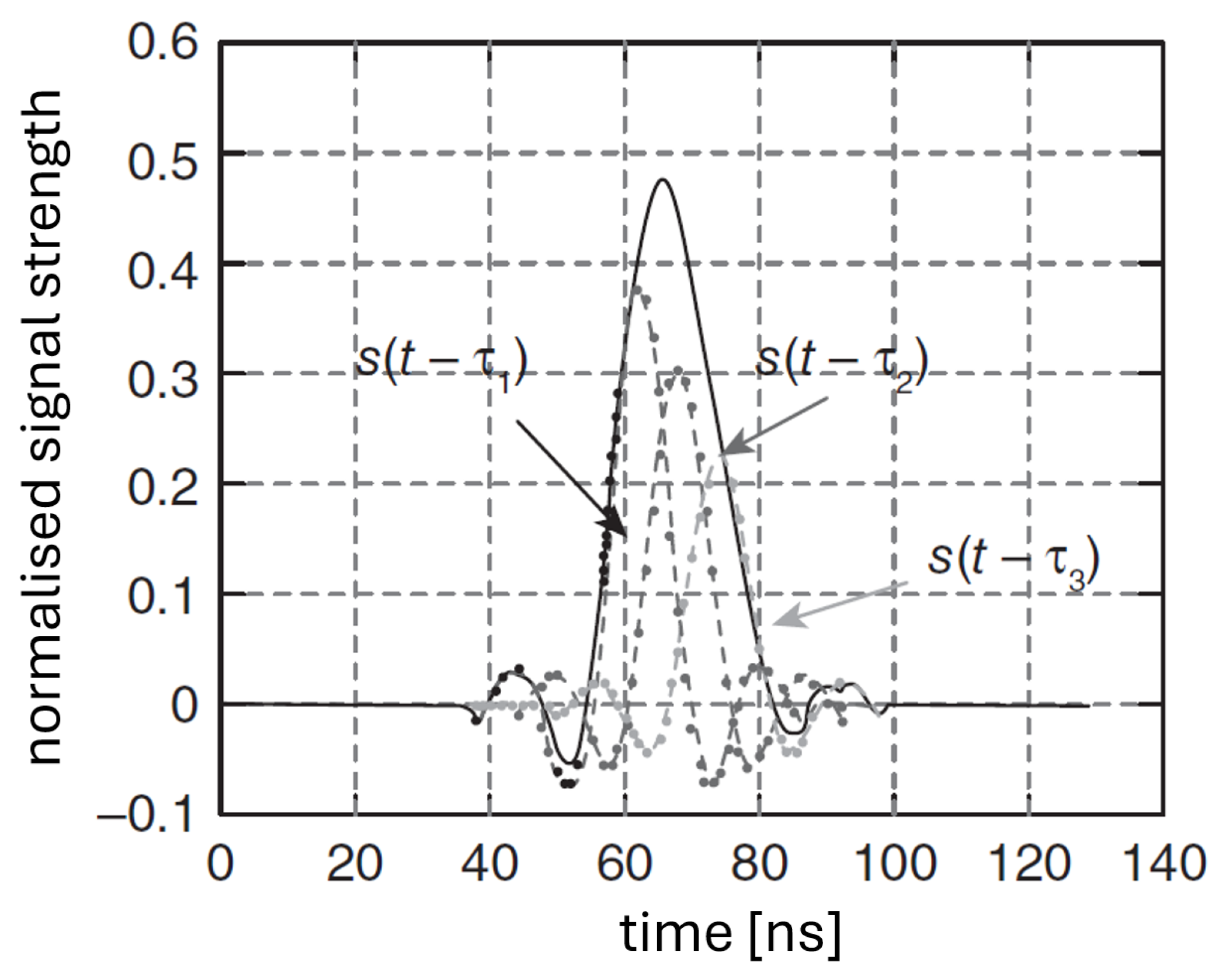
Techniques based on TOA are the most impacted by this phenomenon, as they rely on signal propagation distance to determine the user’s location. In fact, when employing time-based positioning methods, the overlap of MPCs at the receiver is a significant source of error, especially when the time delay of the MPCs is shorter than the inverse of the signal bandwidth. This is illustrated in Figure 2, which shows the arrival of two more MPCs with a delay less than the length of the signal pulse.

2.3. Noise

Noise impairs the performance of TOA-based methods, with the accuracy of time-delay estimates proportional to the signal-to-noise ratio (SNR). Different approaches exhibit varying degrees of resilience to the SNR, with the traditional matched filter maximum likelihood (MFML) TOA estimator suffering from fast accuracy degradation when the SNR drops below a predefined threshold [19]. High SNR and wide bandwidth lower the theoretical lower bound of the position estimate accuracy [20]. In the case of GNSS, the signals are narrow band and usually have a low SNR when reaching the receiver, resulting in poor accuracy. Consequently, despite higher carrier frequencies suffering from increased power attenuation, the high available bandwidth in 5G NR positioning improves the accuracy of radio-based positioning based on TOA estimation.

2.4. 5G Deployment

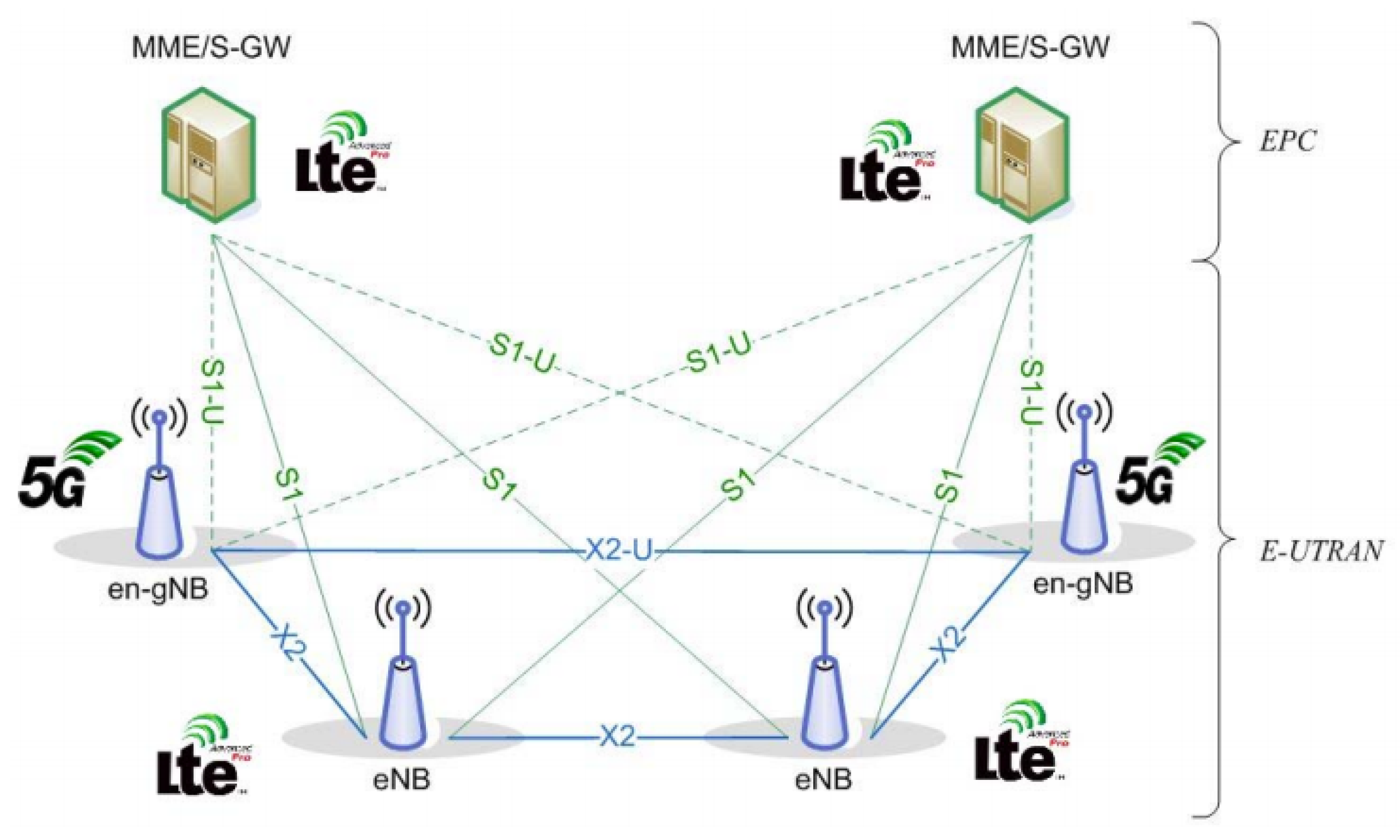
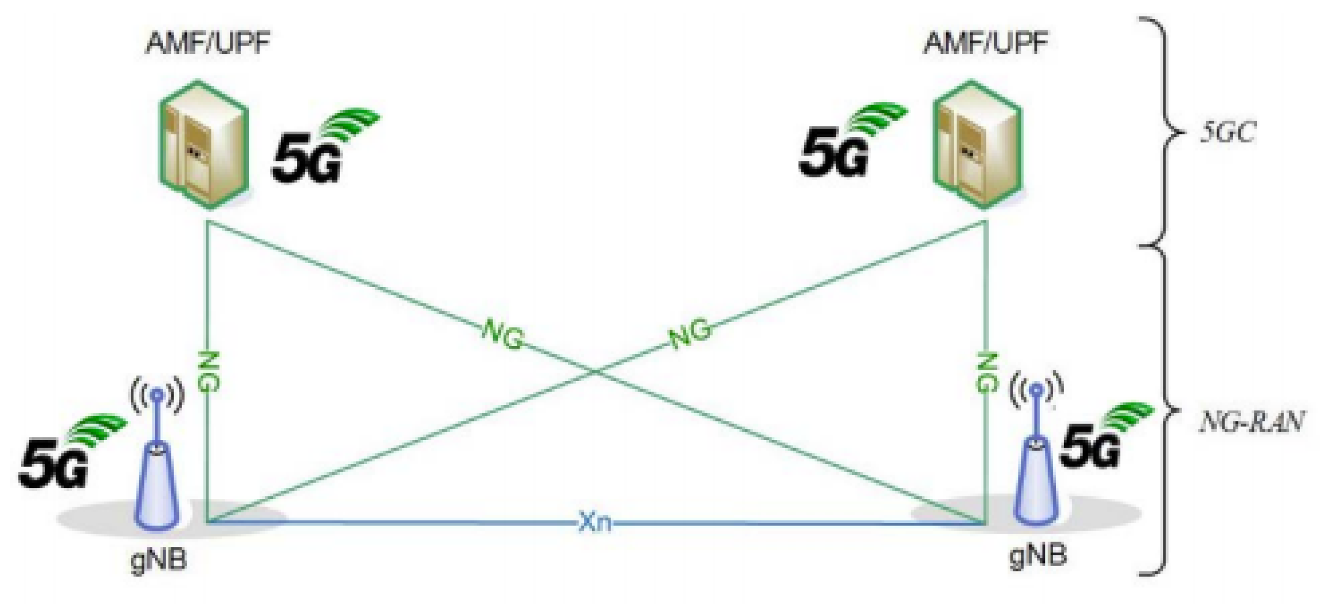
The 3GPP Release 15 announced two deployment phases for the 5G cellular network in 3GPP TR 21.915 [21]. The initial phase of 5G deployment is the so-called NSA architecture illustrated in Figure 3, which combines the 5G radio access network (RAN) and its NR interfaces with the existing LTE and evolved packet core (EPC) infrastructure to provide 5G NR without the need for network replacement to support air mobility [22]. The second phase corresponds to the deployment of the full 5G SA architecture illustrated in Figure 4. Frequency bands for 5G NR are divided into two categories, namely, FR1 and FR2, respectively, termed the sub-6 GHz and mm-Wave bands [23]:
  • cm-Wave 5G: Many of the frequency bands in FR1 overlap with those utilised for 4G and other mobile communication services. The FR1 band was initially designated to bands below 6 GHz, but has now been expanded to 7.125 GHz in anticipation of further spectrum allocations [24].
  • mm-Wave 5G: The frequency bands of FR2 range from 24.25 GHz to 52.6 GHz. At mm-Wave frequencies, significant attenuation losses can be compensated by using massive hybrid arrays [25]. Multipath sparsity in both the temporal and spatial domains is a crucial characteristic of mm-Wave signal propagation, which is caused by the rapidly decreasing energy of reflected mm-Wave signals, with only MPCs with few reflections being able to convey significant power.

2.5. 5G NR Positioning

Fifth-generation positioning has been recently explored with cm-Wave and mm-Wave transmission, confirming that 5G standalone systems are capable of dm and cm level positioning accuracy [26]. Many benefits of 5G infrastructure are inherited in 5G positioning, including the following:
  • Bandwidth availability: Large bandwidth enables higher multipath resolution, translated to higher accuracy for TOA-based positioning. LTE offers a maximum bandwidth of 20 MHz, resulting in expected position errors above 63 m on 95% of the cases [27]. As shown in Table 1, the 5G network will enable bandwidths up to 100 and 400 MHz in the FR1 and FR2 bands, respectively, which can be increased up to 1 GHz using carrier aggregation techniques.
  • Network density: 5G will provide better positioning accuracy by offering a range of access points for transmitting positioning pilot signals and processing user location. Rural macro cells may offer a wide coverage area because of favourable propagation conditions at sub-6 GHz frequencies in rural areas. In contrast to cm-Wave signals, mm-Wave signals are more likely to be obstructed by obstacles, and the probability of receiving NLOS signal components substantially decreases. However, mm-Wave signals suffer from significant attenuation, requiring the deployment of tiny (small, pico, and femto) cells.
  • MIMO and beamforming: MIMO antenna systems are known for achieving high spectral efficiency in wireless communication systems. This is achieved by performing parallel transmissions and increasing the number of antennas at the BS to increase the directivity of the transmitted signal. This reduces the effect of having substantial side lobes, as illustrated in Figure 5, which leads to higher spectral efficiency.
The 5G NSA employs the same positioning techniques as 4G. However, it introduces new and enhanced techniques in release 16. The more relevant techniques are hereby listed:
  • Downlink time difference of arrival (DL-TDOA): This scheme is not fundamentally new and already existed in 4G under the name of Downlink OTDOA. It involves comparing the time difference of arrival between synchronous BSs at the receiver side. The main difference with 5G is that BSs can broadcast their own location on a broadcast channel in the 5G network, allowing the user to autonomously locate itself without the need to send measurements to the network [29].
  • Multicell round-trip time: Under this method, the user must broadcast a location request to several BSs, including the serving and neighbouring BSs. The user location is then computed using the multi-RTT positioning technique. This method eliminates the need for time synchronisation, but is more susceptible to multipath positioning errors since it is a two-way communication.
  • Downlink angle of departure (DL-AOD): This technique relies on DL—positioning reference signal (PRS)—reference signal received power (RSRP) measurements of downlink radio signals from numerous NR transmission/reception points (TRPs) obtained at the user, as well as knowledge of the downlink radio signals’ spatial information and TRPs’ geographical coordinates.
  • Uplink angle-of-arrival (UL-AOA): The measured azimuth and zenith of arrival at numerous TRPs of uplink signals broadcasted from the user are used in the UL-AOA positioning technique. The TRPs utilise assistance data from the positioning server to measure the A-AOA and Z-AOA of the received signals, and the results are combined with other configuration information to estimate the user’s location.

2.6. RF Fingerprinting

Signal-strength-based localisation methods are usually less precise than TOA-based positioning, but can be deployed with little or no change to existing networks. In fact, the statistical model presented in (1) is often used with lateration techniques to predict the location of the user. This approach is termed a model-based technique as it utilises a standard channel model to establish a functional relationship between the RSS and the distance between the transmitter and receiver. In many instances, statistical models are unable to capture the complex relationship between RSS and the receiver distance to a given BS. Thus, this technique is not suitable for applications with accurate positioning requirements. Furthermore, RSS-based positioning experiences more shadowing fluctuation as multipath fading increases. Nonetheless, the significant variability of multipath signals may be used to link each location to its own RF signature, termed an RF fingerprint [16]. The greater the variation in signal strength across various grids of a given scenario, the more varied fingerprints can be observed, resulting in enhanced location accuracy. The fingerprinting resolution can be strengthened if each user can supply its measured multipath delay profile.
Two categories of RF fingerprints exist, namely, the reference fingerprint, collected during offline training, and the target RF fingerprint, taken during the online phase of operations. The number of signal characteristics of an RF fingerprint must be large and diverse enough to allow for a unique RF signature of a particular location reference. At each given location, the chosen signal characteristics must have minimal time variability. However, they will not be steady over time. Even though using mean values decreases small-scale fluctuations, changes or updates in the RAN (such as the insertion of new cells, modifications in the node configuration, or output power variations) may corrupt the RF signature of a specific location. In such cases, the offline fingerprint database must be updated. The RF fingerprinting process is, therefore, divided in two phases:
  • Offline training phase: A correlation database or “radio map” is built, containing a collection of RF signatures, using either radio propagation modelling or field measurements. Each signature is unique and associated with location data.
  • Online localisation phase: During this phase, the signature of interest from the received signal is correlated with the database using a pattern-matching algorithm to estimate the geographic coordinates of the user based on the received signature.

2.7. Neural Networks and Bayesian Regularisation

NNs are powerful tools that enable a network of neurons to learn patterns during a training phase, allowing them to predict outputs for new inputs based on learned data. They consist of nonlinear parametric functions dependent on input features, adjustable weights, and biases. Overfitting and underfitting are two key issues that frequently arise in ML. Overfitting occurs when a model is too closely tailored to the training data, leading to poor generalisation, while underfitting happens when the model is too simplistic, failing to capture the relationship between inputs and outputs. Techniques like early stopping, regularisation, hyperparameter tuning, and data collection can mitigate these issues [30].
Bayesian regularisation (BR) is a well-known method that helps overcome overfitting issues in an NN. This determines the optimal combination of squared errors and weights for building a network model that generalises well, with a cost function described by (3):
J ( w ) = β n = 1 N | | y ( x n , w ) y t | | 2 + α n = 1 N e n 2
where β and α are the hyperparameters or regularisation parameters, N corresponds to the quantity of training data, and { x n } and { y t } are the inputs and target values, respectively. BR adds a weight decay, E w = n = 1 N e n 2 , to the objective function for artificial NNs, which penalises high weights in the hopes of achieving improved generalisation. The weight decay coefficient promotes small values of w and reduces the tendency of a model to overfit. The left side of (3) provides information about the goodness of fit of the model. Therefore, the trade-off during the training phase lies between (1) maximising the influence of E w by minimising the value of α such that α β , and (2) betting on the goodness of a fit at the expense of model complexity by maximising the value of β such that β α [31].

2.8. Ensemble Learning

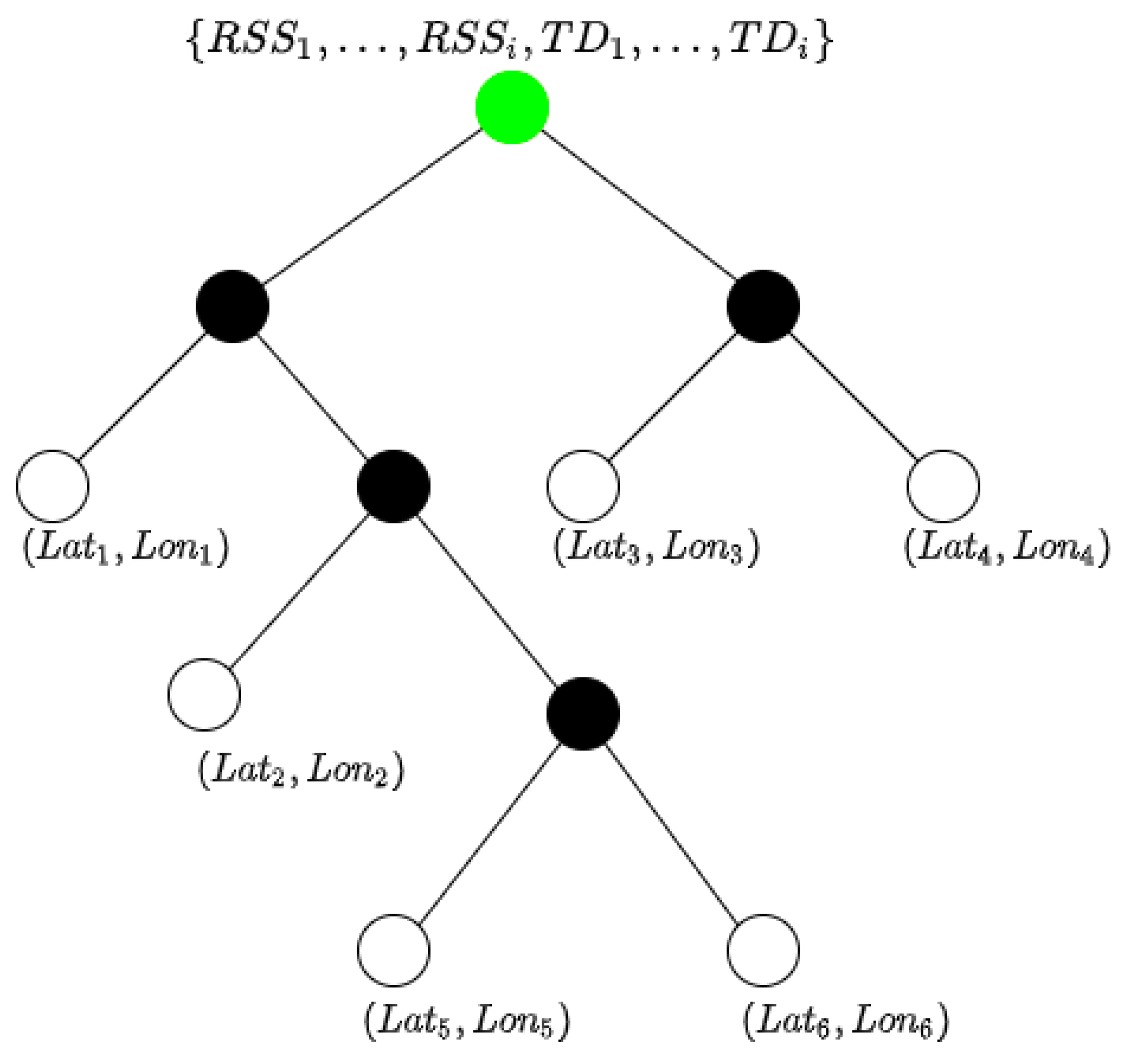
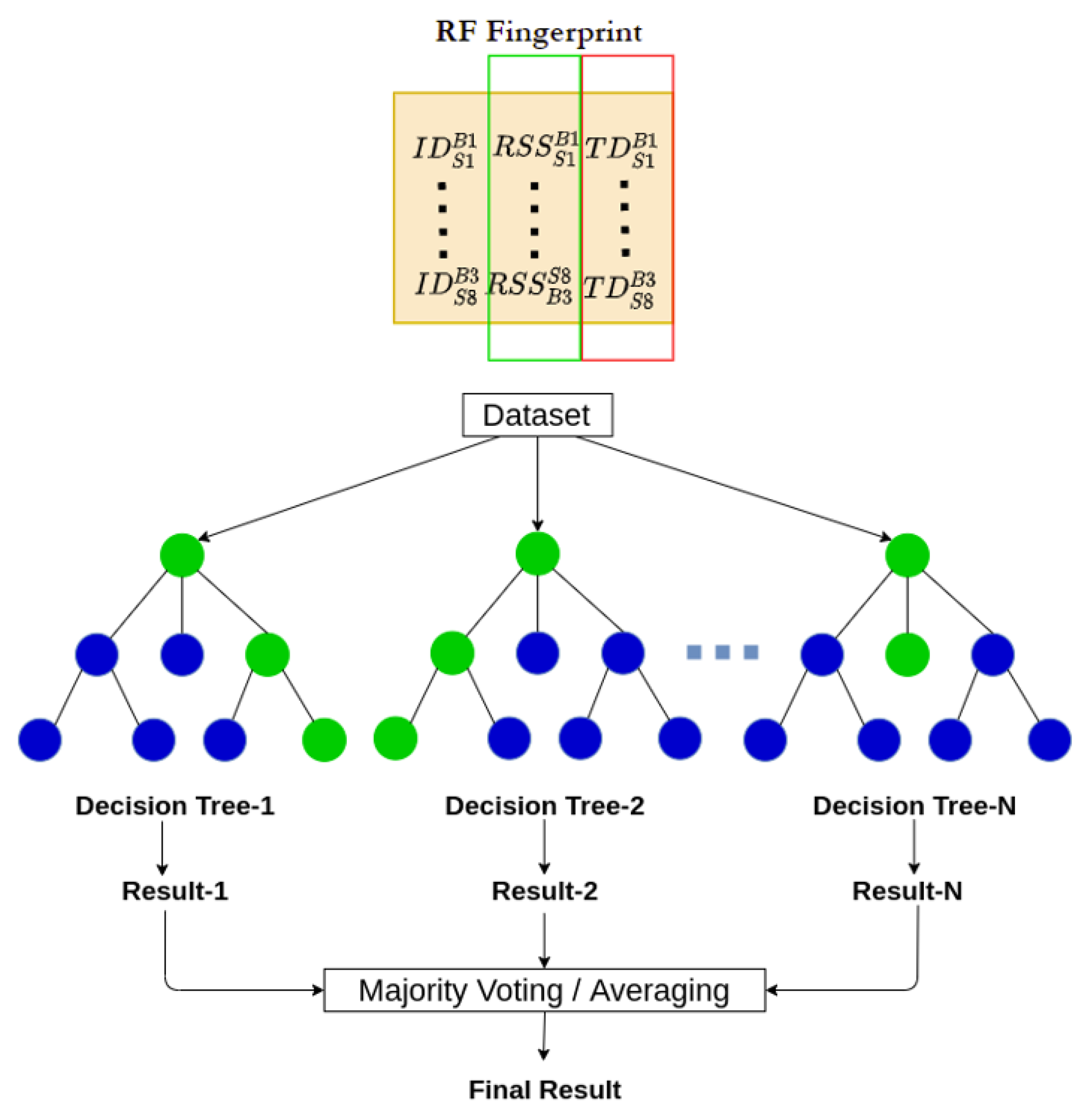
Ensemble learning employs tree-based models as supervised learning tools widely used in classification and regression problems. The objective is to separate the input dataset into distinct classes using binary judgments of the features in the input set. In Figure 6, the tree splits the input space { R S S , T D } using binary decisions to estimate the output { L a t , L o n } . It begins at the root node (green) and works its way up the tree until it comes across a leaf, with the number of nodes crossed in the tree’s longest route determining its depth. The ensemble model’s basic concept is that a number of weak learners join forces to produce a strong learner. A technique commonly used in ensemble learning to reduce the variance of a decision tree is bagging or bootstrap aggregation. The goal is to construct multiple subsets of data from a training sample selected randomly, with each subset forming a small learner. The average of all predictions from the different trees is then used, being more reliable than a single decision tree. This approach handles higher dimensional data very well, but results in lower accuracy regression predictions since the final prediction is dependent on the mean predictions from subset trees.

2.9. Machine Learning for Localisation

In recent years, the progress of AI has fuelled a movement towards improving outdoor and indoor localisation using AI and ML. Numerous studies introduce ML models such as support vector machines [32], decision trees [33], random forests, and NNs [34] to solve localisation and positioning [13] problems. Notably, Ref. [11] combined decision tree regression and a two-layer deep NN (DNN) to achieve a mean positioning error of 1.4 m. Due to multipath effects, however, signal strength estimates for a specific location suffer from a significant degree of fluctuation over time. Consequently, Ref. [35] suggested that channel state information (CSI) measurements provide a much better understanding of the multipath profile.
Most of the literature to date is focused on 5G mm-Wave positioning. When the number of GNSS visible satellites is fewer than four, Ref. [8] proposed a GNSS-5G hybrid positioning algorithm which combines GNSS TOA and 5G AOA information. This results in an accuracy improvement of 5 m in 95% of the cases compared to when standalone 5G AOA positioning is used to locate a user. Ref. [5] proposed a novel algorithm based on MUSIC for NLOS propagation called NC-MUSIC. To detect and cancel the NLOS signal, this method employs cross-correlation. The number of MPCs is then estimated and the noise subspace is extracted using an unsupervised multipath estimation approach. For OTDOA, TOA, AOA, and other 5G positioning techniques, this algorithm offers high-precision time delay estimates, which greatly improves 5G positioning accuracy in urban areas.

3. Methodology

This section describes the methodology employed to model the 5G environment and develop novel 5G cm-Wave positioning techniques. The methodology used to create the offline correlation database is first presented, before outlining two ML-based approaches for matching patterns during the online learning phase of RF fingerprinting.

3.1. Overview

RF fingerprinting is based on the principle that signal propagation varies depending on the surrounding environment. These variations—caused by factors such as building reflections, signal scattering, and multipath interference—create a unique “fingerprint” for each location. By capturing these signal features, such as RSS and TOA, and associating them with known coordinates, a comprehensive database can be created that serves as the foundation for accurate real-time positioning. When new signal measurements are received during real-time operations, the system compares these measurements to the stored fingerprints in the database, allowing the user location to be estimated based on the best match.
Advanced ray-tracing simulations are first used to create a comprehensive RF fingerprint database. Signal features such as RSS and TOA are collected from multiple locations in the target urban environment. These signal characteristics are recorded alongside their corresponding geographic coordinates, creating a detailed map of signal behaviour across the area of interest. These ray-tracing simulations model how 5G NR signals propagate in complex urban environments, taking into account reflections, diffractions, and obstructions caused by buildings and other structures.
During real-time operations, the system receives new signal measurements from the air vehicle as it moves through the urban environment. These measurements are compared against the pre-constructed RF fingerprint database. By identifying the fingerprint that most closely matches the current signal characteristics, the system can accurately estimate the vehicle’s position. This process is repeated continuously as the vehicle moves, providing real-time, high-precision location tracking. In this work, two supervised learning algorithms are trained for online matching of signal characteristics to geographical coordinates.

3.2. Offline Training Phase

This section outlines the methodology used to build the correlation database for RF fingerprinting. The RF fingerprint at a given location i = { 1 , , M } is given by (4):
F P i = I D 1 R S S 1 T D 1 I D N R S S N T D N
where I D j is the cell identification of the j-th next generation node (gNB), R S S j and T D j are the received signal strength and time delay of the signal, respectively, M is the number of location samples, and N represents the number of anchors within the range of the reference location. This process involves gathering measurable parameters of the signal which are correlated with the the sample location to ensure the uniqueness of each RF fingerprint.
In this work, the RSS and round-trip delay are considered, since they are parameters already measured by common cellular devices. Additionally, the delay spread is considered to assess the total ray components received at a given reference point. Specifically, the city of London was chosen to analyse the performance of a standalone 5G positioning system. Ray-tracing was then used to collect ray data as a function of geographical location.

3.2.1. Modelling Software

The ray-tracing software WinProp was used to simulate radio propagation in a 3D model of a portion of the city of London. WinProp provides a very accurate and quick wave propagation model together with a radio network planning component for cellular networks, including LTE and 5G. The WallMan software package was first used to generate a vector building database from the opensource OpenStreetMap file of the selected environment [36]. The ProMan software package was then used to predict path loss between the gNBs and reference locations.

3.2.2. Urban Environment Model

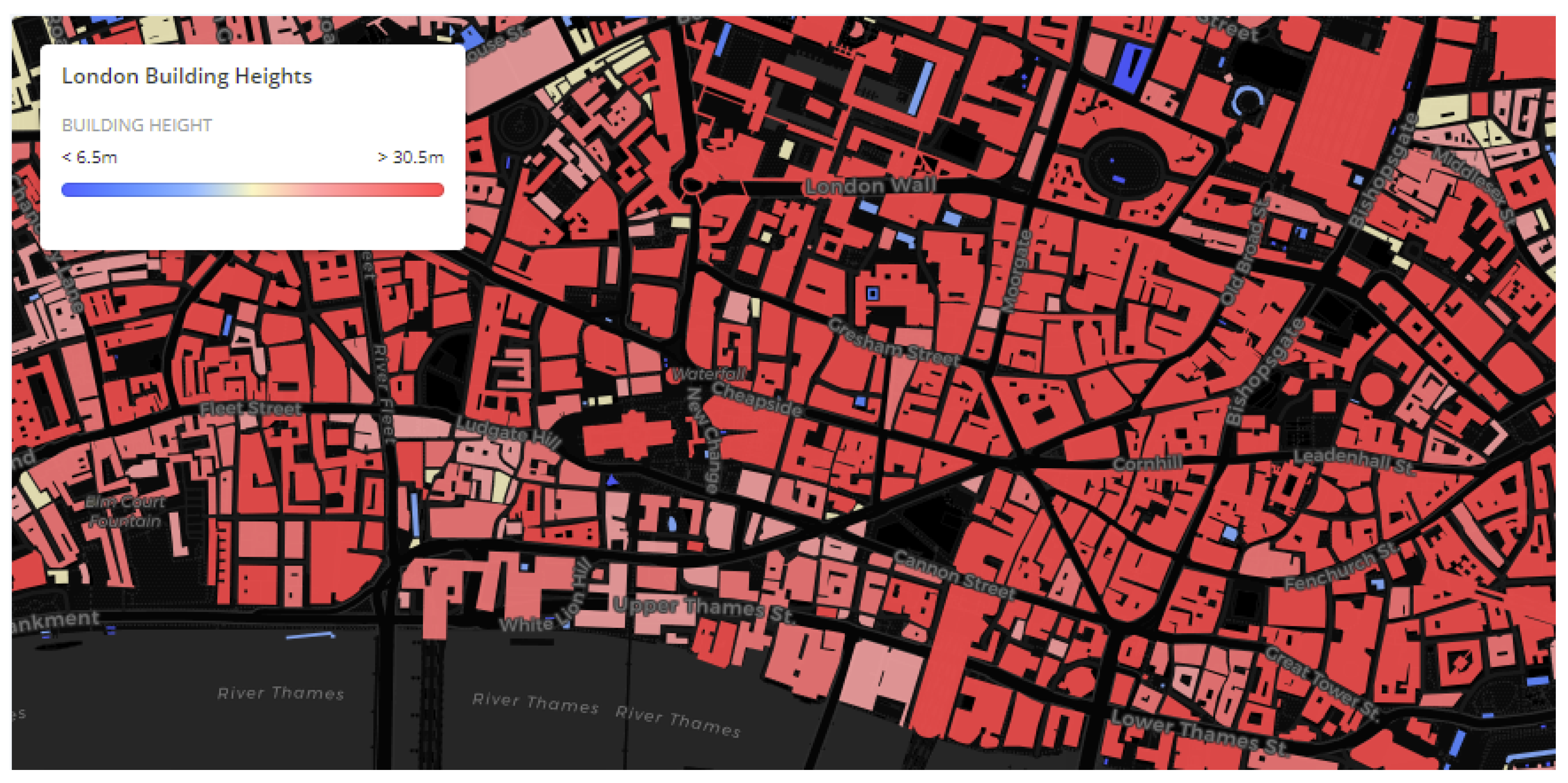
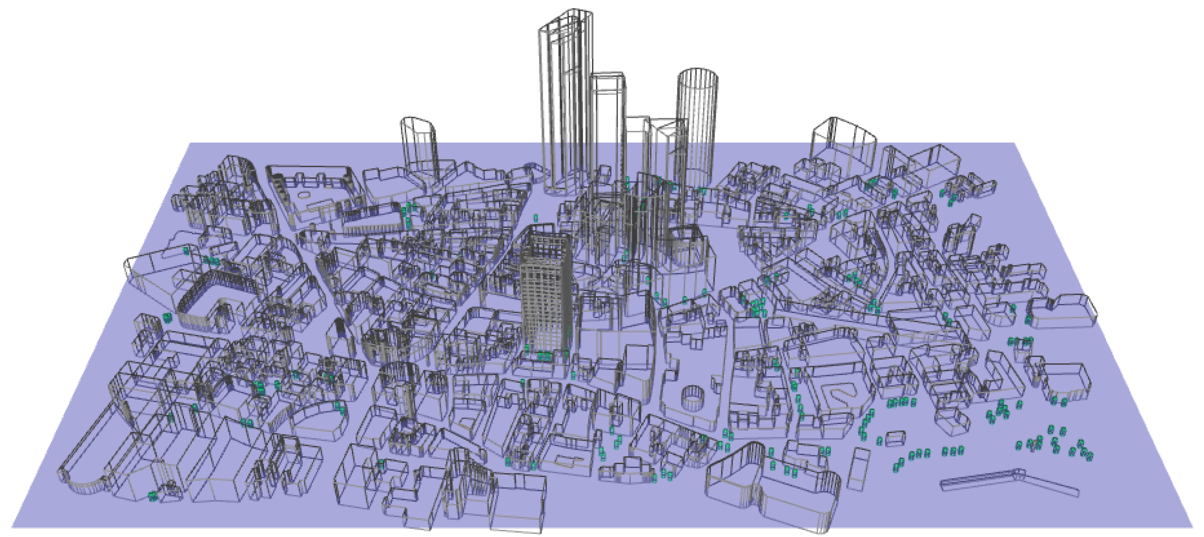
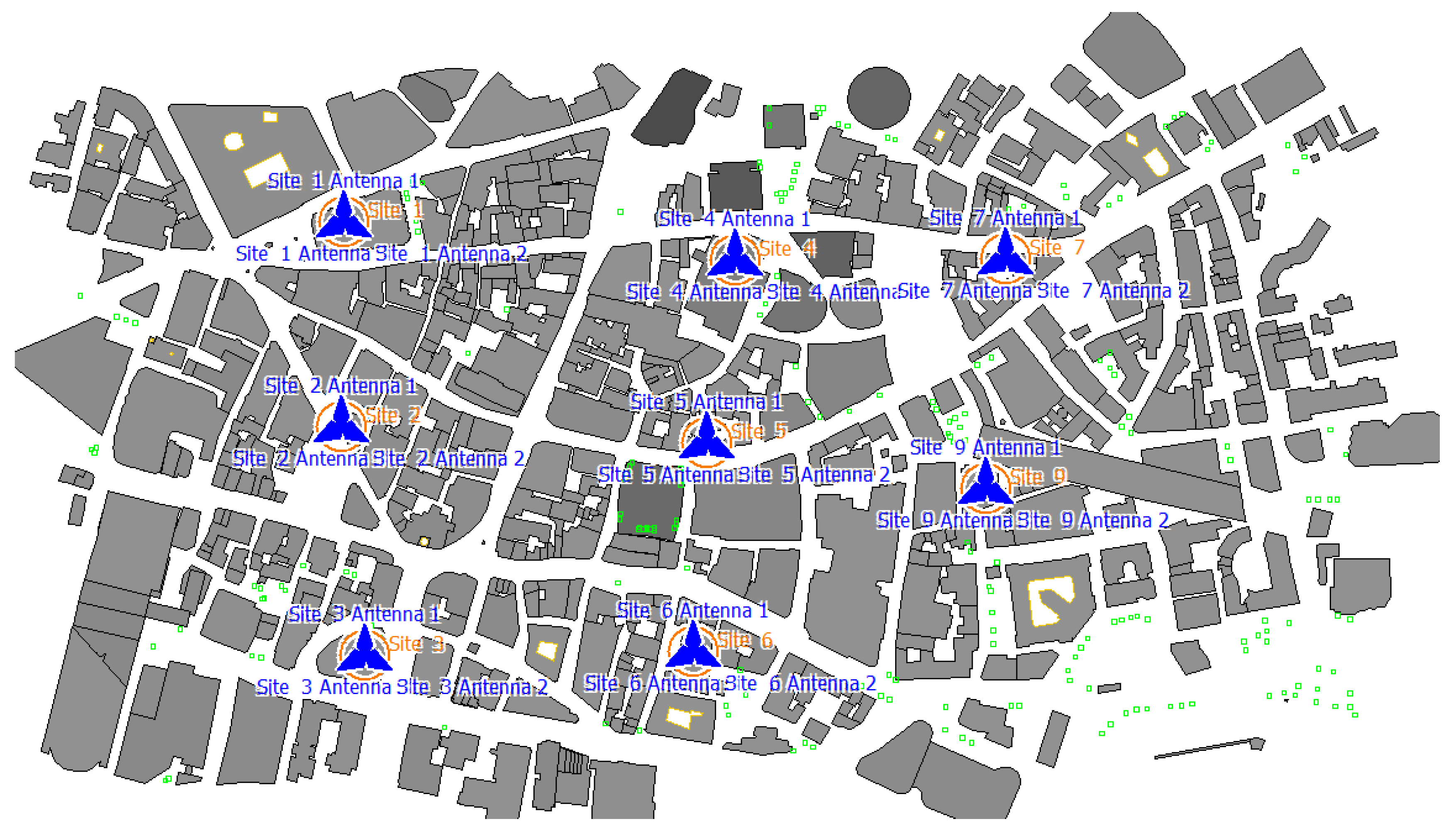
The portion of the city of London illustrated in Figure 7 was chosen due to its high average building height of approximately 31.9 m. The urban scenario was converted to a series of 3D building vectors, with each building described as a vertical cylinder with polygonal ground planes. Figure 8 shows the 3D profile of the urban scenario. Table 2 and Figure 9 further show the BS station configuration and other relevant parameters related to the antenna configuration. A three-sector configuration was chosen for the BSs with a spacing orientation of 120° between sectors.

3.2.3. Air Interface Model

The air interface includes all the information related to the type of access, duplex mode, carrier frequency, bandwidth, coding, and required signal-to-noise-and-interference ratio (SNIR) at the receiver. In this work, the air interface file for 5G networks offered by Altair within the modelling software application was used and modified to include the n78 (3300 to 3800 MHz) band of interest, as the most widely tested and deployed 5G frequency in several countries. Specifically, a carrier frequency of 3550 MHz and a bandwidth of 100 MHz were considered. Additionally, a numerology μ = 2 was selected, corresponding to a sub-carrier spacing of Δ f = 2 μ = 60 kHz. Table 3 summarises the air interface parameters.

3.2.4. Antenna Pattern

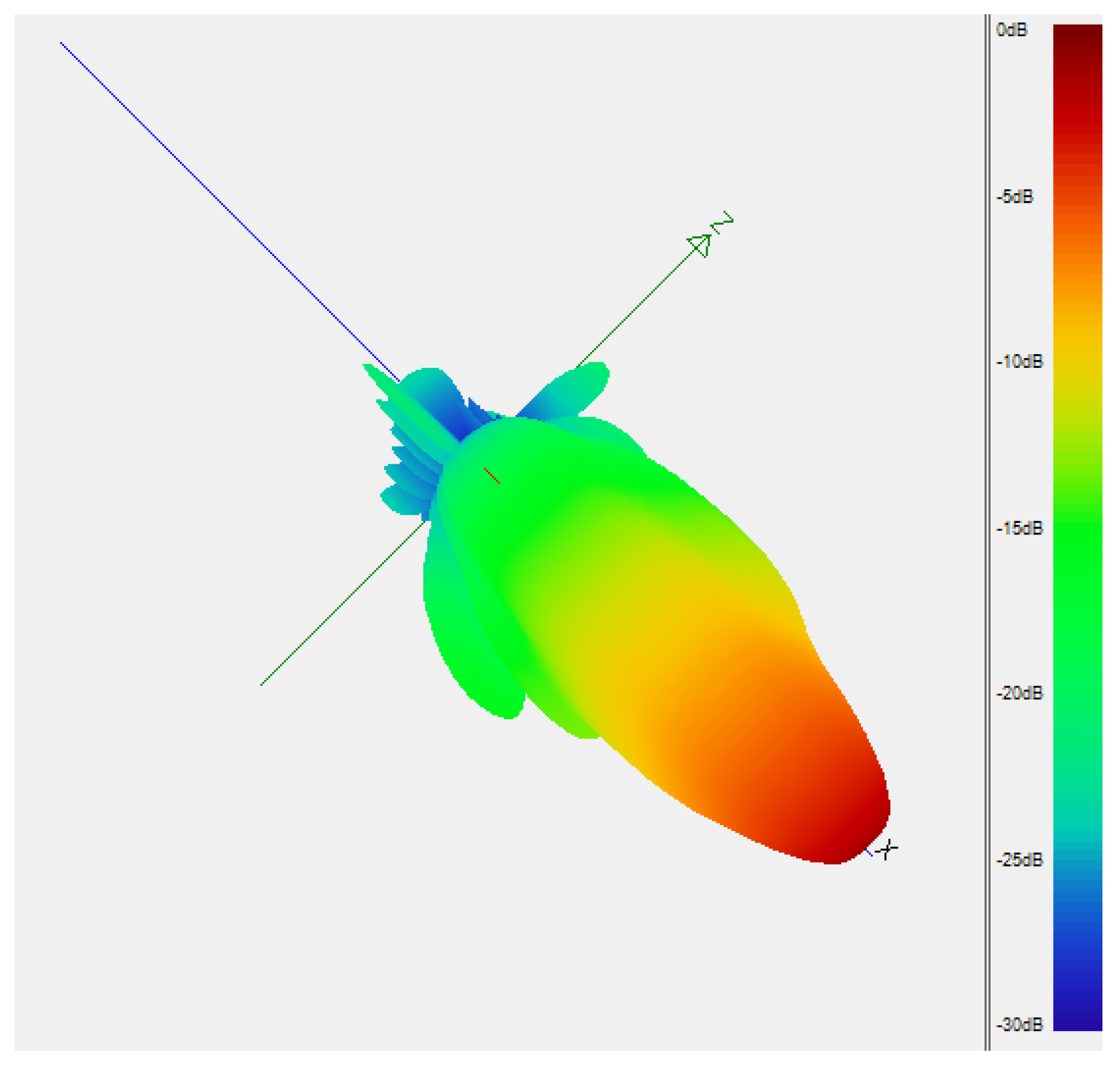
Fifth-generation networks use directional antennas, with the antenna pattern file used in this work obtained from the UBIQUITY open source antenna pattern files. Each sector is equipped with a 15.5 dB gain antenna, having the radiation pattern depicted in Figure 10. For simplicity, one directional beam per sector was considered.

3.2.5. Correlation Database

A correlation database obtained by propagation modelling allows for simple, quick, and low-cost updates. If the RAN elements change, an updated database can be simply created through an updated model simulation. Nonetheless, the resulting location precision is expected to be lower than that obtained through field measurements. Two approaches are hereby considered:
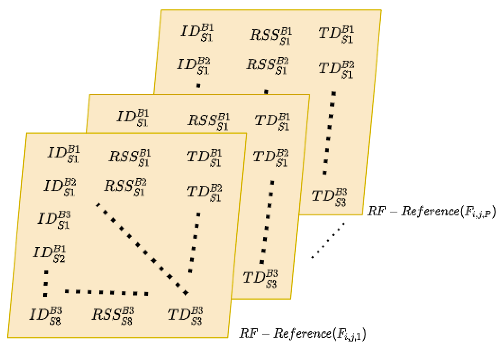
  • In the first approach, a unique correlation database is built containing the full search space for RF fingerprinting, by storing the measured data in a multidimensional matrix, where each dimension corresponds to the measured RSS and the time delay of the beams from anchors in the range of the reference point, as illustrated in Figure 11. Each 2D-array F i , j corresponds to a specific geographic location, P is the number of locations processed, I D i corresponds to the ID of each single beam per BS, and  R S S i and T D i are the strongest beam RSS and time delay from the i-th BS, respectively. Because each sector has a unique beam pattern, there is no need to filter observations from low RSS beams. When a multibeam pattern is utilised, data should be filtered to consider only those beams with a higher RSS. Information from low-RSS rays may be inaccurate, adding complexity to the algorithms while only providing minor performance improvements.
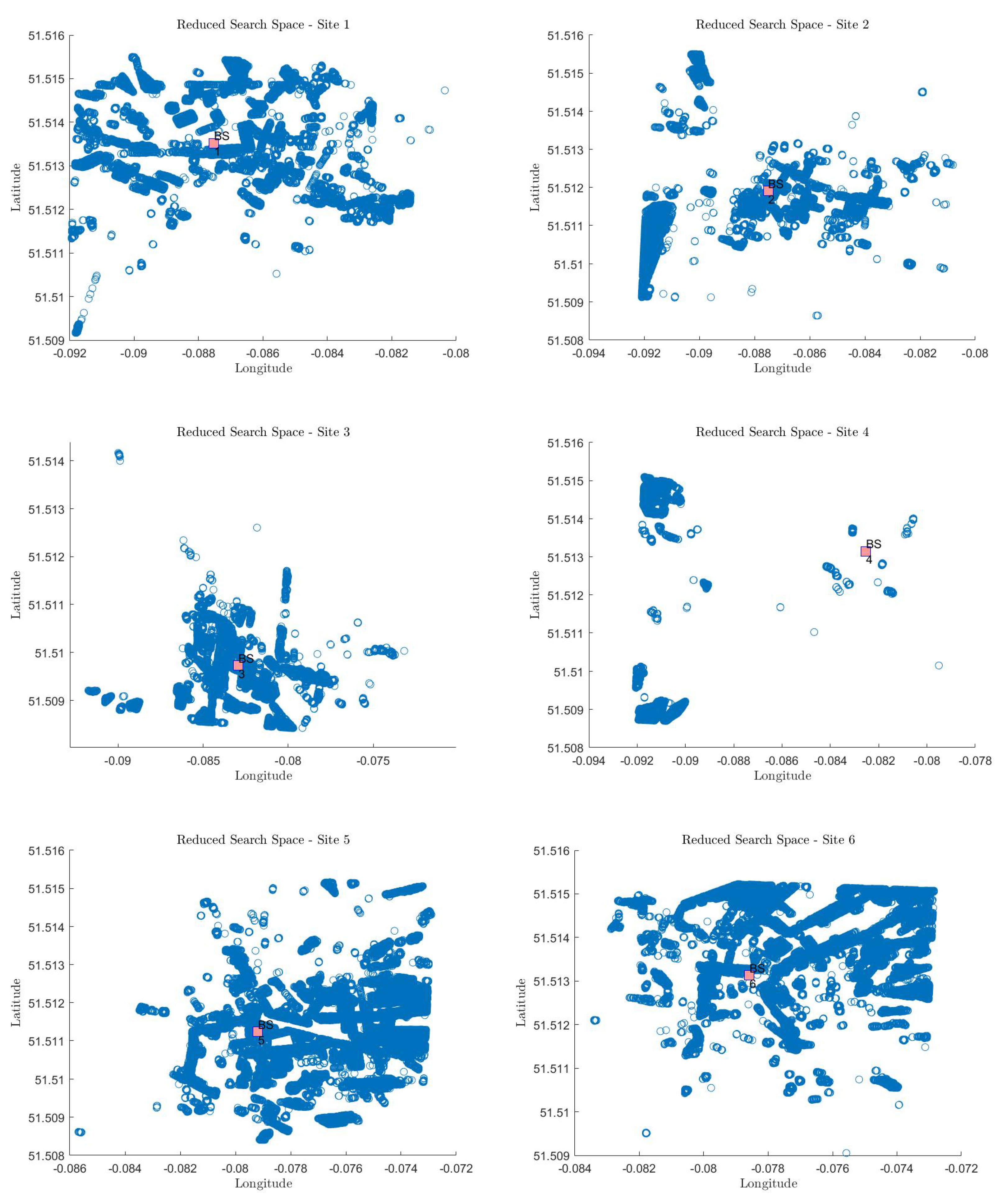
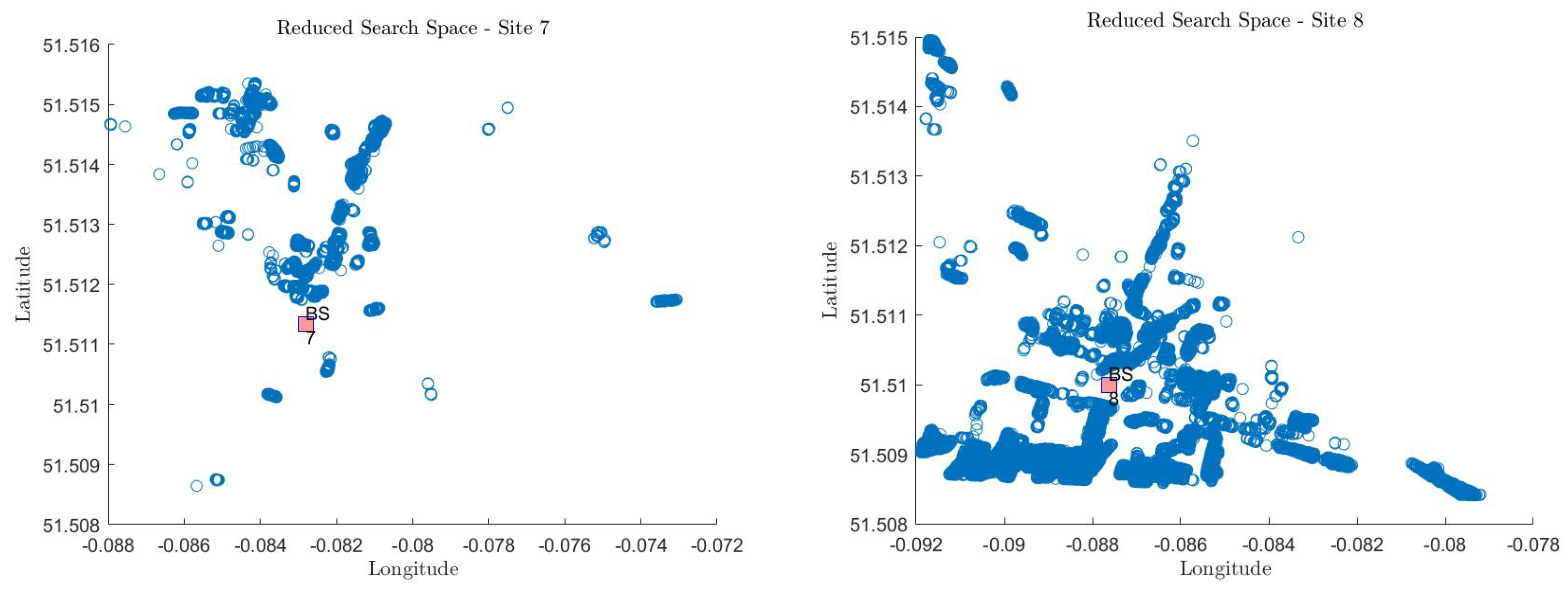
  • In the second approach, a correlation database for each serving cell is developed, in which the serving BS makes the prediction. This technique takes advantage of the ability of cellular devices to determine the strongest received beam and initiate a handover procedure to partition the initial complete search space A into several smaller search spaces B, as illustrated in Figure 12, each of which corresponds to a particular service area. This produces N sub-matrices, where N is the number of BSs and each sub-matrix is associated with a specific service area, accomplished by sorting each RF-Reference in such a way that R S S i = R S S k if i = k to obtain (5):
    B = { ( L a t i , L o n i , F i , j ) | A , F i , j ( 1 , 1 ) = F P ( 1 , 1 ) }

3.3. Online Localisation Phase

During the online phase, online measurements are matched against entries in the database to provide a prediction of the user location. To address the location problem, two supervised learning techniques are hereby proposed to map locations to the RF fingerprints stored in the database. This assumes that trained matching models are integrated within the location management (LM) function of the 5G Core, and that the user can send measurements of the RSS and time delay at a predefined rate when multipath signals are resolvable.

3.3.1. NN-Based Approach

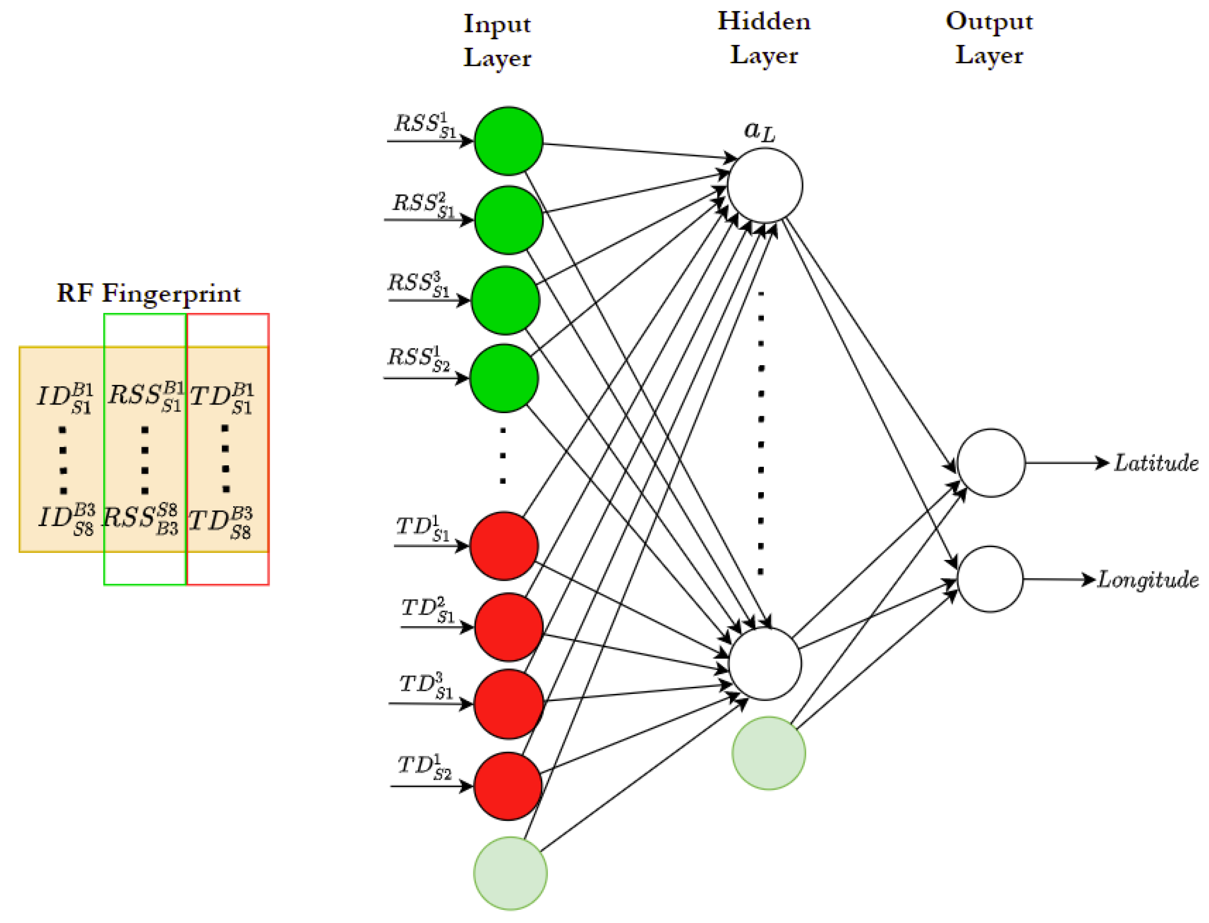
The first approach utilises BRANNs. The topology of the selected NN has 48 inputs and 2 neurons in the output layer with rectified linear unit (ReLU) activation functions, as illustrated in Figure 13. This is reduced to 24 inputs when just four neighbouring gNBs are considered or when solely considering RSS measurements. Additionally, RSS and time delay features are first normalised to a range of [0, 1] using min–max scaling, according to (6):
X n o r m = X X m i n X m a x X m i n
The optimal size of the hidden layer was determined through conventional optimisation techniques both for individual serving areas, and for the whole serving area when using the full space search approach.

3.3.2. Random Forest

The second approach leverages regression learning algorithms to train a random forest algorithm, as illustrated in Figure 14 (Algorithm 1). In this case, the number of trees in the random forest and the depth of each tree are optimised to identify the optimal tree configuration for each scenario. The advantage of this approach is its immunity to overfitting, eliminating the need to delete features that are highly correlated. Additionally, ensemble tree-based algorithms can handle high-dimensional input variables and work on large datasets. In this work, multiple models were trained using between 1 and 200 regression trees, and the configuration with the lowest root mean square error (RMSE) on the validation set was selected as the candidate configuration. A minimum leaf count of 1 was also assumed.
Algorithm 1 Random forests [37]
  1:
Generate N learners:
  2:
for  n = 1 , 2 , , N   do
  3:
     Sample randomly the dataset A to produce A n .
  4:
     Create root node R N n containing A n
  5:
     Call CreateTree( R N n )
  6:
end for
  7:
if  R N includes only instances of a single class then return
  8:
else
  9:
      Select x randomly of the possible splitting features in R N
10:
      To split on, choose the feature F with the largest information gain
11:
      Create F child nodes for R N , R N 1 , , R N j , where F can take on any number of
12:
      values ( F 1 , , F k )
13:
      for  j = 1 , , k  do
14:
          Set the contents of R N j A j , where A j represents all instances in R N that
15:
       corresponds to F j .
16:
       CreateTree( R N j )
17:
      end for
18:
end if

4. Testing and Evaluation

This section describes the metrics selected to evaluate the performance of the developed algorithms. The dataset generated from the modelling software is subsequently analysed to investigate the correlation between measurements from different gNBs. The proposed learning algorithms are then evaluated and thoroughly discussed.

4.1. Evaluation and Analysis Metrics

4.1.1. MSE and RMSE

Two types of error metrics are often used to report the performance of a regression model, namely, the mean squared error (MSE) and RMSE, described by (7) and (8), respectively:
M S E = 1 N n = 1 N ( y n y ^ n ) 2
R M S E = M S E
where { y n } is the n-th expected value of the dataset and { y ^ n } is the n-th predicted value.

4.1.2. Pearson Correlation Coefficient

Correlation coefficients are used to determine the linear dependency of two random variables. Specifically, the Pearson correlation coefficient is defined as (9) when each variable has N scalar observations, or as (10) in terms of covariance:
ρ ( X , Y ) = 1 N 1 i = 1 N X i μ X σ X Y i μ Y σ Y
ρ ( X , Y ) = c o v ( X , Y ) σ X σ Y
where { σ } and { μ } are the standard deviation and mean of the variables X and Y, respectively. The correlation matrix of N random variables can, therefore, be expressed as (11):
M = ρ ( X 1 , X 1 ) ρ ( X 1 , X N ) ρ ( X N , X 1 ) ρ ( X N , X N )

4.2. Dataset and Feature Analysis

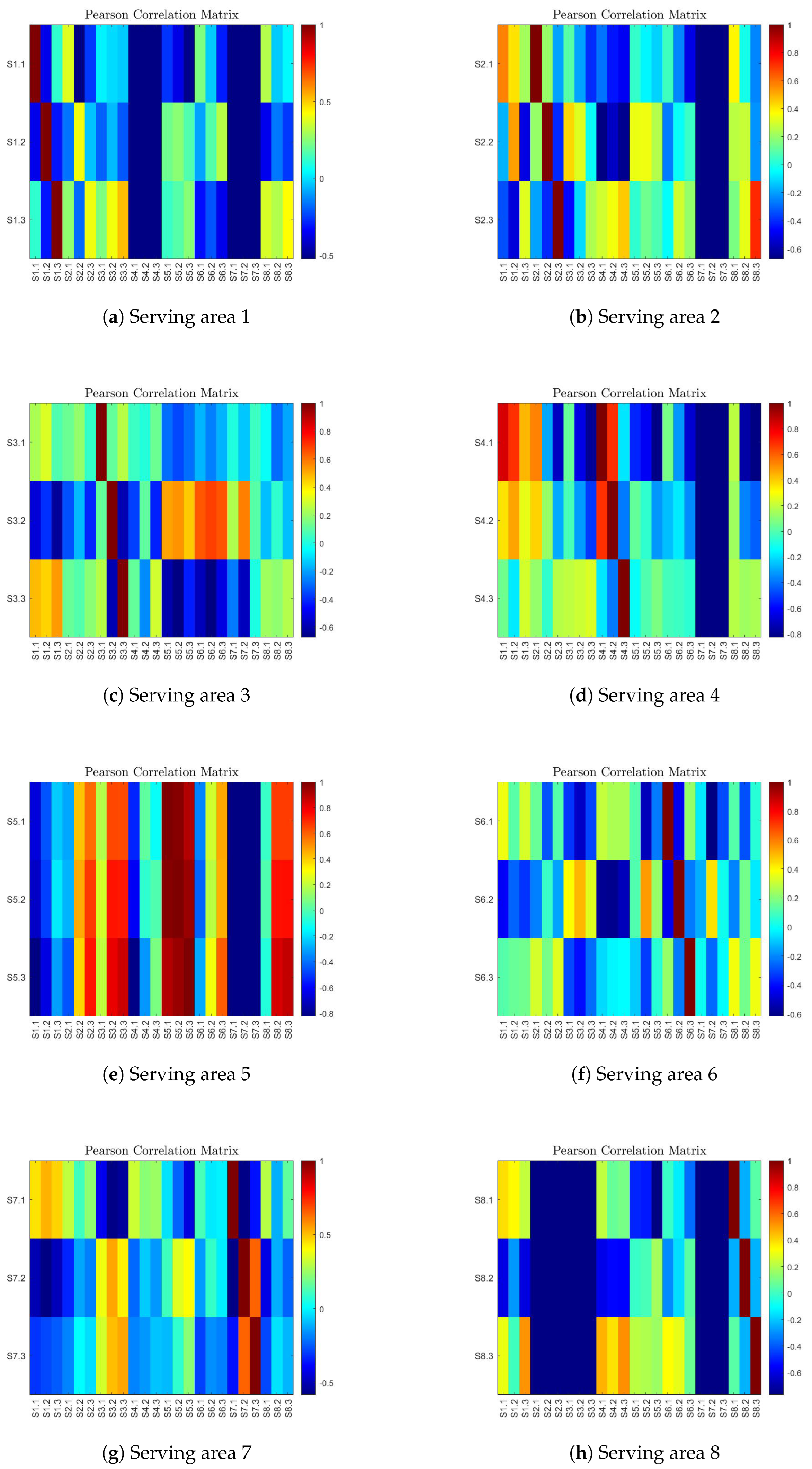
The Pearson coefficient was used to analyse the linear correlation between input features of the NN, and avoid performance degradation due to multicollinearity by removing redundant input variables. Specifically, features that presented a correlation above an 85% threshold were excluded from the dataset before training the BRANN model. In contrast to NN algorithms, random forests are immune to multicollinearity because the algorithm itself assesses the predictors’ importance during training.
Figure 15 shows the correlation between the RSS measurements from the serving BS and those from neighbouring BSs across the whole database. As illustrated in Figure 15c, for instance, there is a high correlation between RSS readings from S6, S5, and S7 in Area 3, which may be explained by the geometry of the beam’s transmission and the closeness of the sites. The same analysis was conducted on the features for all areas studied in this work.

4.3. Bayesian Regularisation NN Results

The MATLAB trainbr function was used to train the NN models to be hosted in the LM of the 5G core. The original dataset containing the RF fingerprint for each service area was randomly divided into training and testing subsets in the ratio 0.9:0.1, respectively. Initially, the network was trained using solely RSS observations, before being trained using both RSS and time delay features. Table 4 lists the optimal hidden layer size for each service area, with which the resulting position RMSE was minimised.
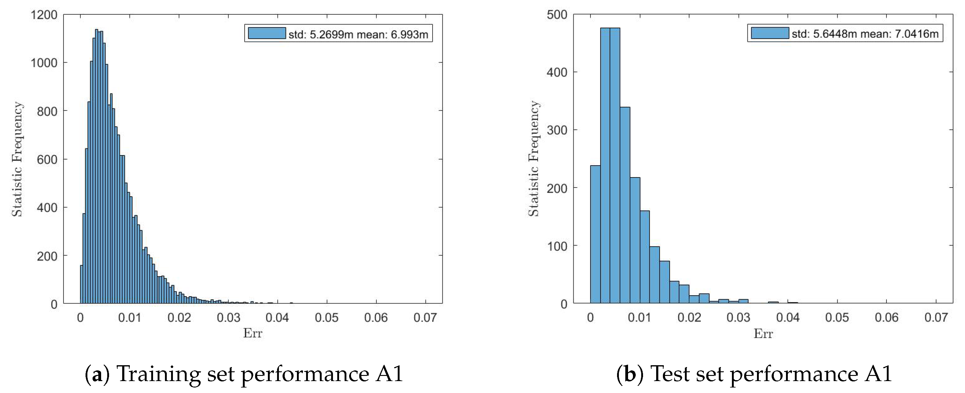
The performance of algorithms was also shown to improve when additional time delay information was included. Such information, however, is only available under LOS conditions or when multipath signals are resolvable. Figure 16a illustrates the error in the position prediction after training the network with 90% of the dataset available for Area 1, which includes the beam’s signal strength measurements and the corresponding time delay of the ray associated with that beam. Conversely, all performance discussions are based on the accuracy of the test set. In the case of Area 1, the error in the prediction decreased by 29.89% and 28.90%, respectively, in the training and test datasets when the TOA information was available, regardless of whether the signal corresponded to an NLOS or LOS component. Similar results were observed for service areas 2–8, but are hereby omitted for brevity.
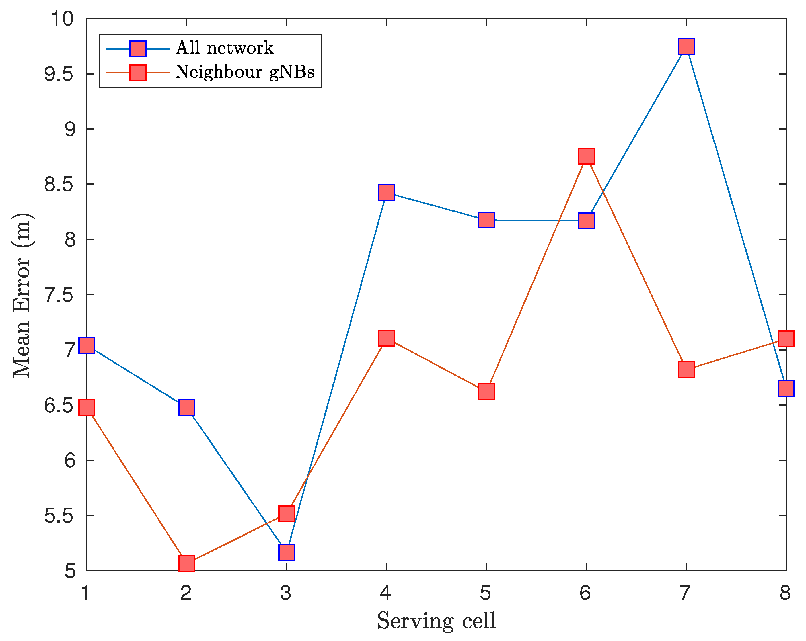
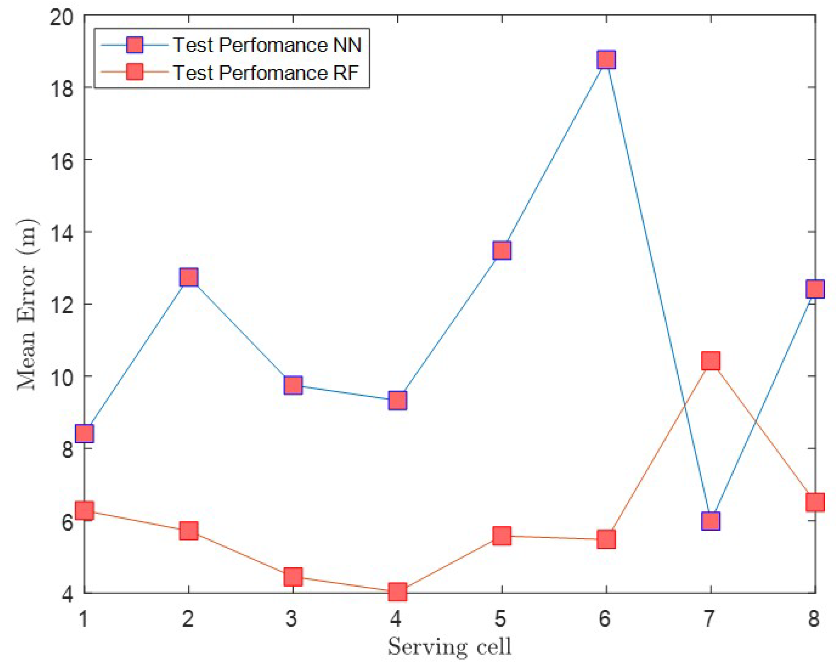
The initial hypothesis was that areas with a large dataset would generalise better than those with a smaller one, as NN performance often improves with larger datasets. This was not the case, however, in the conducted experiments, as the models for servicing regions with a larger dataset (such as areas 5 and 6) exhibited lower accuracy than those with a smaller sample size (such as areas 4 and 7), as listed in Table 5. Dimensionality reduction was further applied in subsequent experiments. Instead of considering the features of the strongest beams across all gNBs of the testbed scenario, only the strongest beams of the closest neighbouring gNBs were considered. This approach successfully reduced training time, while performing more accurately in most service cells, as shown in Figure 17.

4.4. Random Forest Results

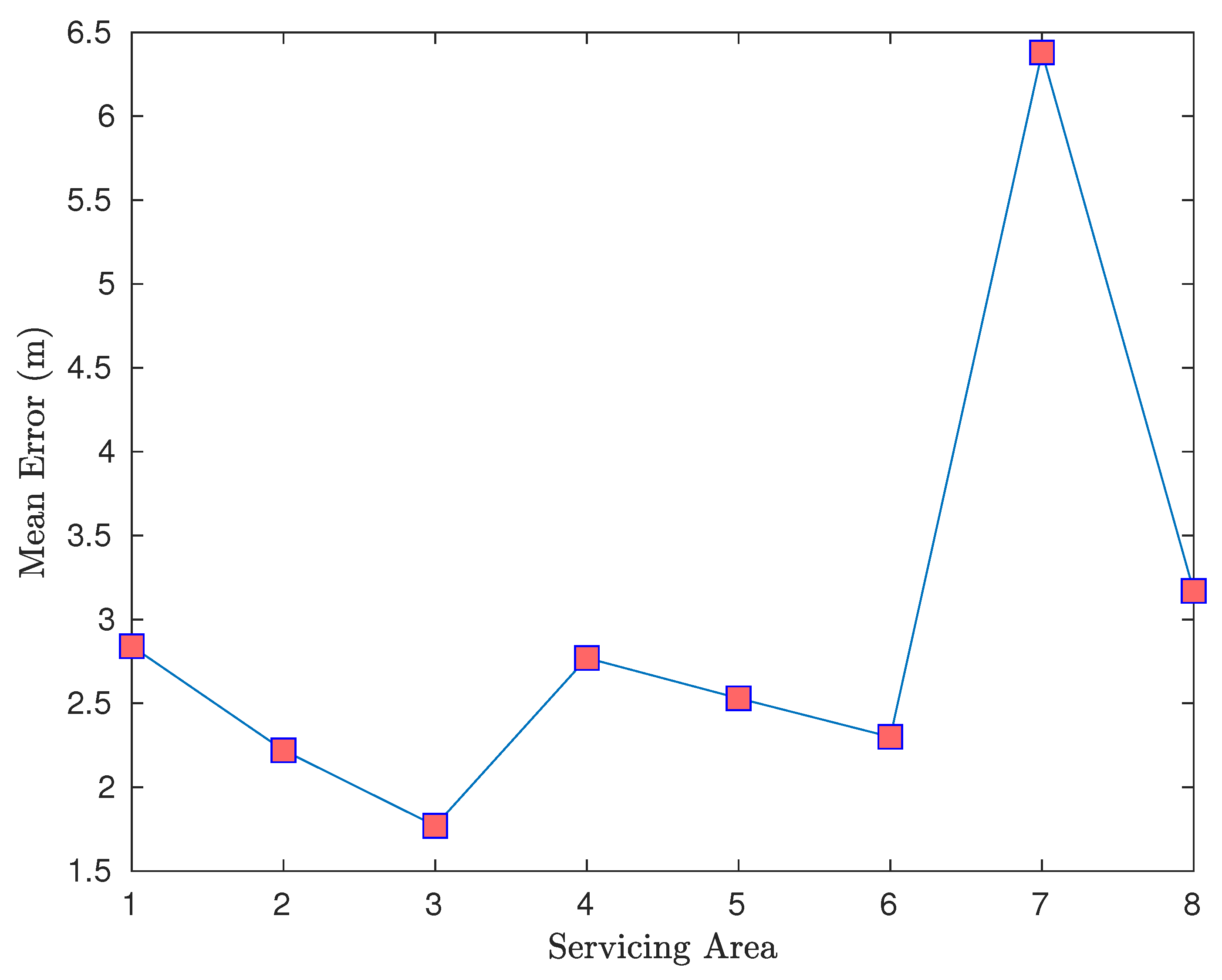
The same dataset, constructed based on sample locations, was used to train a random forest, which exhibited better results than those obtained using the NN-based approach. Figure 18 illustrates the performance of the prediction on the test dataset for each service area. Notably, except for service areas 7 and 8, all models exhibited a mean error under 3 m. By varying the number of estimators in the forests, the performance of random forests models may also be improved further.
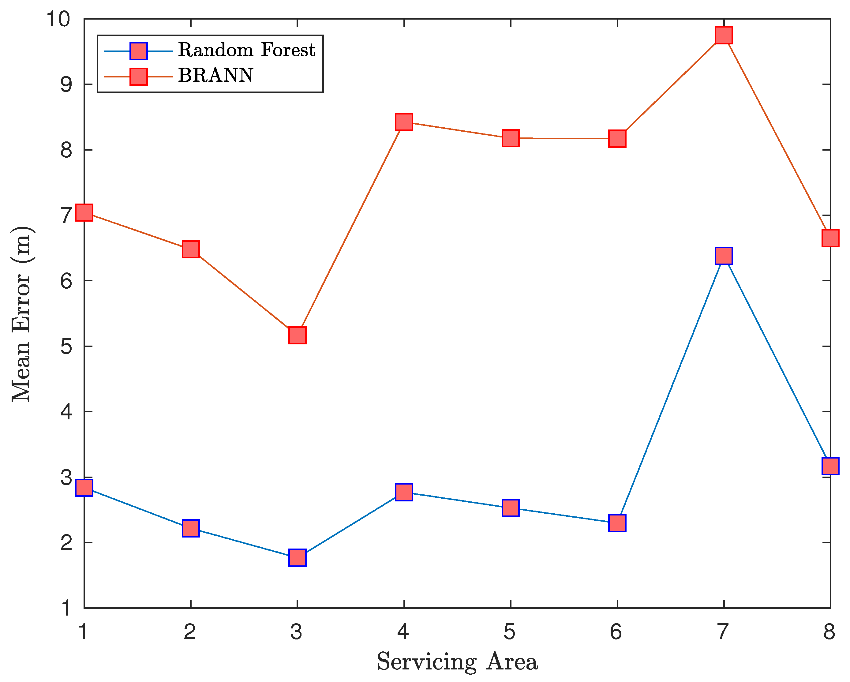
Figure 19 and Figure 20 demonstrate the performance of the BRANN and random forest models. The random forests model outperformed the BRANN model on the same dataset. Additionally, it was more computationally efficient, requiring less training time. Nonetheless, while random forest approaches have a finite improvement factor, the NN approach allows for greater flexibility in improving the performance observed in this study.

5. Conclusions

5.1. Summary

Fifth-generation technology holds significant promise for both outdoor and indoor positioning. The 5G FR2 band, however, faces high-frequency signal attenuation, necessitating additional access points. Consequently, the sub-6 GHz band, particularly the n78 frequency range (3.5 GHz), is the primary frequency considered for global 5G deployment. This study, thereby, focused on the sub-6 GHz range, specifically utilising RF fingerprinting for vehicle positioning. Using WinProp, a radio map of a section the city of London was created, and ray-tracing techniques were leveraged to create a correlation database for the specified area. NN- and random-forest-based algorithms were subsequently trained to predict positions using signal strength and time delay data. The random forest model achieved an accuracy of less than 3 m in six out of eight regions, outperforming the BRANN model. The results demonstrate that RF fingerprinting combined with random forests can offer good performance accuracy for positioning applications, even when solely relying on readily available RSS and time delay measurements.

5.2. Future Work

This work assumed location samples on the XY plane at a constant height, thus restricting the available dataset. Future work should extend the model to the XYZ dimension by sampling signals from different heights and considering additional layers in the 3D model. This could transform the problem into a classification task, enabling the use of novel ML approaches to increase positioning accuracy. Exploring the use of beam ID information at reference locations could further enhance model performance. Additionally, future research should focus on implementing an algorithm to classify ray components as LOS or NLOS, improving models that rely on TOA by adding this component type as a feature. This enhancement could reduce bias in areas where different component types reach neighbouring samples.

Author Contributions

Conceptualization, I.M. and S.A.-R.; methodology, I.M.; software, I.M.; validation, I.M.; formal analysis, I.M. and C.C.; investigation, I.M.; resources, S.A.-R.; data curation, I.M.; writing—original draft preparation, C.C.; writing—review and editing, C.C. and S.A.-R.; visualization, C.C.; supervision, S.A.-R. and G.I.; project administration, G.I. All authors have read and agreed to the published version of the manuscript.

Funding

This research received no external funding.

Data Availability Statement

Data are contained within the article.

Conflicts of Interest

The authors declare no conflicts of interest.

Abbreviations

The following abbreviations are used in this manuscript:
4GFourth generation
5GFifth generation
AIArtificial intelligence
AOAAngle of arrival
BRBayesian regularisation
BRANNBayesian regularised artificial neural networks
BSBase station
CRBCramer–Rao low bound
CSIChannel state information
DAADetect and avoid
DL-AODDownlink angle of departure
DL-TDOADownlink time difference of arrival
DNNDeep neural network
EASAEuropean Union Aviation Safety Agency
EPCEvolved packet core
FRFrequency range
gNBNext generation node
GNSSGlobal navigation satellite systems
INSInertial navigation system
ITSIntelligent transportation system
LMLocation management
LOSLine of sight
LTELong-term evolution
MFMLMatched filter maximum likelihood
MIMOMultiple input multiple output
MLMachine learning
MPCMultipath component
MSEMean squared error
NLOSNon-line of sight
NNNeural network
NRNew radio
NSANonstandalone
PBNPerformance-based navigation
PRSPositioning reference signal
RANRadio access network
RFRadio frequency
ReLURectified linear units
RMSERoot mean squared error
RSRPReference signal received power
RSSReceived signal strength
RSSIReceived signal strength indicator
RTTRound trip time
SAStandalone
SNIRSignal-to-noise-and-interference ratio
SNRSignal-to-noise ratio
TDOATime difference of arrival
TOATime of arrival
TRPTransmission/reception points
UAMUrban air mobility
UASUnmanned aircraft system
UAVUnmanned aerial vehicle
UL-AOAUplink angle-of-arrival

References

  1. Wanniarachchi, S.T.; Turau, V. A study on the influence of 5G network planning on communication in Urban Air Mobility. In Proceedings of the 2023 IEEE 24th International Symposium on a World of Wireless, Mobile and Multimedia Networks (WoWMoM), Boston, MA, USA, 12–15 June 2023; pp. 394–399. [Google Scholar] [CrossRef]
  2. Warrier, A.; Aljaburi, L.; Whitworth, H.; Al-Rubaye, S.; Tsourdos, A. Future 6G communications powering vertical handover in non-terrestrial networks. IEEE Access 2024, 12, 33016–33034. [Google Scholar] [CrossRef]
  3. EASA. Study on the Societal Acceptance of Urban Air Mobility in Europe; European Union Aviation Safety Agency: Cologne, Germany, 2021. [Google Scholar]
  4. Shu, Y.; Xu, P.; Niu, X.; Chen, Q.; Qiao, L.; Liu, J. High-rate attitude determination of moving vehicles with GNSS: GPS, BDS, GLONASS, and Galileo. IEEE Trans. Instrum. Meas. 2022, 71, 5501813. [Google Scholar] [CrossRef]
  5. Deng, Z.; Zheng, X.; Wang, H.; Fu, X.; Yin, L.; Liu, W. A novel time delay estimation algorithm for 5G vehicle positioning in urban canyon environments. Sensors 2020, 20, 5190. [Google Scholar] [CrossRef]
  6. Rastorgueva-Foi, E.; Costa, M.; Koivisto, M.; Talvitie, J.; Leppäneny, K.; Valkama, M. Beam-based device positioning in mmWave 5G systems under orientation uncertainties. In Proceedings of the 2018 52nd Asilomar Conference on Signals, Systems, and Computers, Pacific Grove, CA, USA, 28–31 October 2018; pp. 3–7. [Google Scholar] [CrossRef]
  7. Yuan, Z.; Guo, W.; Al-Rubaye, S. Multi-UAV wireless positioning using adaptive multidimensional scaling and extended kalman filter. In Proceedings of the 2022 IEEE Globecom Workshops (GC Wkshps), Rio de Janeiro, Brazil, 4–8 December 2022; pp. 1437–1441. [Google Scholar] [CrossRef]
  8. Sun, C.; Zhao, H.; Bai, L.; Cheong, J.W.; Dempster, A.G.; Feng, W. GNSS-5G hybrid positioning based on TOA/AOA measurements. In Proceedings of the China Satellite Navigation Conference, Chengdu, China, 23–25 May 2020; Springer: Berlin/Heidelberg, Germany, 2020; pp. 527–537. [Google Scholar]
  9. Peral-Rosado, D.; José, A.; Saloranta, J.; Destino, G.; López-Salcedo, J.A.; Seco-Granados, G. Methodology for simulating 5G and GNSS high-accuracy positioning. Sensors 2018, 18, 3220. [Google Scholar] [CrossRef]
  10. Jagannath, A.; Jagannath, J.; Kumar, P.S.P.V. A comprehensive survey on radio frequency (RF) fingerprinting: Traditional approaches, deep learning, and open challenges. Comput. Netw. 2022, 219, 109455. [Google Scholar] [CrossRef]
  11. Butt, M.M.; Rao, A.; Yoon, D. RF fingerprinting and deep learning assisted UE positioning in 5G. In Proceedings of the 2020 IEEE 91st Vehicular Technology Conference (VTC2020-Spring), Antwerp, Belgium, 25–28 May 2020; pp. 1–7. [Google Scholar]
  12. Whitworth, H.; Al-Rubaye, S.; Tsourdos, A. Urban Air Mobility link budget analysis in 5G communication systems. In Proceedings of the 2023 IEEE 24th International Symposium on a World of Wireless, Mobile and Multimedia Networks (WoWMoM), Boston, MA, USA, 12–15 June 2023; pp. 400–406. [Google Scholar] [CrossRef]
  13. De Sousa, M.N.; Thomä, R.S. Applying random forest and multipath fingerprints to enhance TDOA localization systems. IEEE Antennas Wirel. Propag. Lett. 2019, 18, 2316–2320. [Google Scholar] [CrossRef]
  14. Dong, Y.; Du, B.; Zhang, L. Target detection based on random forest metric learning. IEEE J. Sel. Top. Appl. Earth Obs. Remote Sens. 2015, 8, 1830–1838. [Google Scholar] [CrossRef]
  15. Rappaport, T.S. Wireless Communications: Principles and Practice; Prentice Hall PTR: Upper Saddle River, NJ, USA, 1996; Volume 2. [Google Scholar]
  16. Heon Lee, J.; Michael Buehrer, R. Fundamentals of received signal strength-based position location. In Handbook of Position Location: Theory, Practice, and Advances, 2nd ed.; John Wiley & Sons: Hoboken, NJ, USA, 2018; pp. 369–404. [Google Scholar]
  17. Wang, Y.; Chen, X.; Liu, P. Statistical multipath model based on experimental GNSS data in static urban canyon environment. Sensors 2018, 18, 1149. [Google Scholar] [CrossRef] [PubMed]
  18. Michael Buehrer, R.; Venkatesh, S. Fundamentals of time-of-arrival-based position location. In Handbook of Position Location: Theory, Practice, and Advances, 2nd ed.; John Wiley & Sons: Hoboken, NJ, USA, 2018; pp. 199–236. [Google Scholar]
  19. Apartsin, A.; Cooper, L.N.; Intrator, N. SNR-dependent filtering for time of arrival estimation in high noise. In Proceedings of the 2010 IEEE International Workshop on Machine Learning for Signal Processing, Kittila, Finland, 29 August–1 September 2010; pp. 427–431. [Google Scholar]
  20. Dardari, D.; Conti, A.; Ferner, U.; Giorgetti, A.; Win, M.Z. Ranging with ultrawide bandwidth signals in multipath environments. Proc. IEEE 2009, 97, 404–426. [Google Scholar] [CrossRef]
  21. Release 15 Description—Summary of Rel-15 Work Items. Available online: https://portal.3gpp.org/desktopmodules/Specifications/SpecificationDetails.aspx?specificationId=3389 (accessed on 15 May 2021).
  22. Al-Rubaye, S.; Tsourdos, A. Airport connectivity optimization for 5G ultra-dense networks. IEEE Trans. Cogn. Commun. Netw. 2020, 6, 980–989. [Google Scholar] [CrossRef]
  23. 101-1 NR User Equipment (UE) Radio Transmission and Reception—Part 1: Range 1 Standalone. Available online: https://portal.3gpp.org/desktopmodules/Specifications/SpecificationDetails.aspx?specificationId=3283 (accessed on 30 April 2021).
  24. 5G Frequency Bands, Channels for FR1 & FR2. Available online: https://www.electronics-notes.com/articles/connectivity/5g-mobile-wireless-cellular/frequency-bands-channels-fr1-fr2.php (accessed on 30 April 2021).
  25. Zhang, J.A.; Huang, X.; Dyadyuk, V.; Guo, Y.J. Massive hybrid antenna array for millimeter-wave cellular communications. IEEE Wirel. Commun. 2015, 22, 79–87. [Google Scholar] [CrossRef]
  26. Sobehy, A. Machine Learning Based localization in 5G. Ph.D. Thesis, Institut Polytechnique de Paris, Palaiseau, France, 2020. [Google Scholar]
  27. Medbo, J.; Siomina, I.; Kangas, A.; Furuskog, J. Propagation channel impact on LTE positioning accuracy: A study based on real measurements of observed time difference of arrival. In Proceedings of the 2009 IEEE 20th International Symposium on Personal, Indoor and Mobile Radio Communications, Tokyo, Japan, 13–16 September 2009; pp. 2213–2217. [Google Scholar]
  28. Mousa, M.; Al-Rubaye, S.; Inalhan, G. Unmanned Aerial Vehicle positioning using 5G New Radio technology in urban environment. In Proceedings of the 2023 IEEE/AIAA 42nd Digital Avionics Systems Conference (DASC), Barcelona, Spain, 1–5 October 2023; pp. 1–9. [Google Scholar] [CrossRef]
  29. 3GPP TS 38.305 version 16.1.0 Release—5G; NG Radio Access Network (NG-RAN); Stage 2 Functional Specification of User Equipment (UE) Positioning in NG-RAN. Available online: https://www.etsi.org/deliver/etsi_ts/138300_138399/138305/16.01.00_60/ts_138305v160100p.pdf (accessed on 1 March 2024).
  30. Goodfellow, I.; Bengio, Y.; Courville, A. Deep Learning; MIT Press: Cambridge, MA, USA, 2016. [Google Scholar]
  31. Okut, H. Bayesian regularized neural networks for small n big p data. In Artificial Neural Networks-Models and Applications; InTech Open: London, UK, 2016; pp. 28–48. [Google Scholar]
  32. Chriki, A.; Touati, H.; Snoussi, H. SVM-based indoor localization in wireless sensor networks. In Proceedings of the 2017 13th international wireless communications and mobile computing conference (IWCMC), Valencia, Spain, 26–30 June 2017; pp. 1144–1149. [Google Scholar]
  33. Sánchez-Rodríguez, D.; Hernández-Morera, P.; Quinteiro, J.M.; Alonso-González, I. A low complexity system based on multiple weighted decision trees for indoor localization. Sensors 2015, 15, 14809–14829. [Google Scholar] [CrossRef] [PubMed]
  34. Wye, K.F.P.; Zakaria, S.M.M.S.; Kamarudin, L.M.; Zakaria, A.; Ahmad, N.B.; Kamarudin, K. RSS-based fingerprinting localization with artificial neural network. J. Physics Conf. Ser. 2021, 1755, 012033. [Google Scholar]
  35. Pecoraro, G.; Di Domenico, S.; Cianca, E.; De Sanctis, M. CSI-based fingerprinting for indoor localization using LTE signals. EURASIP J. Adv. Signal Process. 2018, 2018, 1–18. [Google Scholar] [CrossRef]
  36. Open Street Map.osm File Generator. Available online: https://www.openstreetmap.org/#map=5/54.910/-3.432 (accessed on 20 March 2024).
  37. Manikandan, M.; Vijayakumar, P. Improving the performance of classifiers by ensemble techniques for the premature finding of unusual birth outcomes from cardiotocography. IETE J. Res. 2023, 69, 1734–1744. [Google Scholar] [CrossRef]
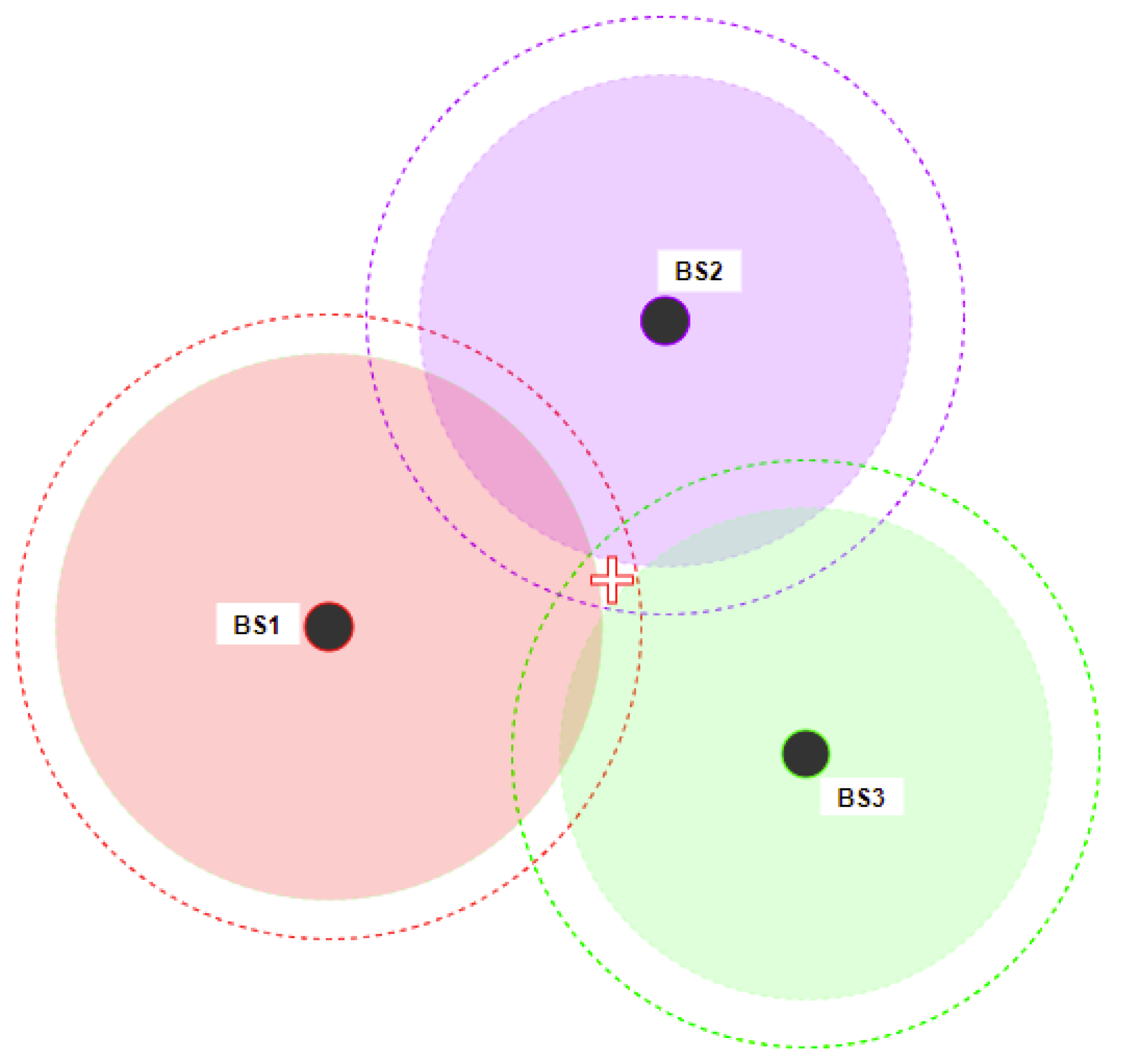
Figure 1. TOA-based positioning.
Vehicles 06 00080 g001
Figure 2. The effect of bandwidths on received MPC [18].
Vehicles 06 00080 g002
Figure 3. 5G NSA architecture [21].
Vehicles 06 00080 g003
Figure 4. 5G SA architecture [21].
Vehicles 06 00080 g004
Figure 5. Antenna number and directivity relationship [28].
Vehicles 06 00080 g005
Figure 6. Five-depth decision tree with binary splits, with a green circle denoting the root node and white circles denoting the end leaves.
Vehicles 06 00080 g006
Figure 7. London building and height profile for selected area.
Vehicles 06 00080 g007
Figure 8. 3D model of the buildings database vector.
Vehicles 06 00080 g008
Figure 9. Urban environment with the BS configuration.
Vehicles 06 00080 g009
Figure 10. 3D model of the UBIQUITY antenna pattern.
Vehicles 06 00080 g010
Figure 11. Correlation database structure.
Vehicles 06 00080 g011
Figure 12. Service areas 1–8.
Vehicles 06 00080 g012aVehicles 06 00080 g012b
Figure 13. Topology of the NN used for online matching.
Vehicles 06 00080 g013
Figure 14. Topology of the random forest algorithm used for online matching.
Vehicles 06 00080 g014
Figure 15. Pearson correlation in serving areas 1 to 8.
Vehicles 06 00080 g015
Figure 16. RSS & TD–BRANN–Frequency Distribution—Area 1.
Vehicles 06 00080 g016
Figure 17. Performance results when using all network measurements and only those of neighbouring gNBs.
Vehicles 06 00080 g017
Figure 18. Mean error per area in the test set using random forests.
Vehicles 06 00080 g018
Figure 19. Results of random forests and BRANN algorithms with both RSS and TD features.
Vehicles 06 00080 g019
Figure 20. Results of random forests and BRANN algorithms with RSS features only.
Vehicles 06 00080 g020
Table 1. 5G NR channel bandwidth.
Frequency RangeFrequency (MHz)Channel Bandwidth (MHz)
FR1410–71255, 10, 15, 20, 25, 30, 40, 50, 60, 80, 90, 100
FR224,250–52,60050, 100, 200, 400
Table 2. System-level BS parameters.
ParameterValue
Nr. sectors3 sectors per site
Tx power40 dBm
Antenna gain15.5 dB
Antenna orientation (azimuth)0 deg
Antenna orientation (downlit)0 deg
Table 3. Ray-tracing parameters.
ParameterValue
ScenarioCity of London
Sites8
Antenna height35 m
FR1 bandn78
Carrier freq.3550 MHz
Numerology2
Planar resolution1 m
Table 4. BRANN optimal hidden layer configurations.
Serving AreaHidden Neurons (RSS and Time Delay)Hidden Neurons (RSS)
15540
23523
35162
43810
55151
66343
75160
85961
Table 5. Mean prediction error per area.
Network Specific
SiteNr. Samples LocationMean RSS and TD [m]Mean RSS [m]
1221467.049.90
2182436.489.74
3215315.169.59
487908.427.46
5570468.1812.67
6417998.1716.83
727569.757.51
8191776.6516.83
Disclaimer/Publisher’s Note: The statements, opinions and data contained in all publications are solely those of the individual author(s) and contributor(s) and not of MDPI and/or the editor(s). MDPI and/or the editor(s) disclaim responsibility for any injury to people or property resulting from any ideas, methods, instructions or products referred to in the content.