Abstract
Autonomous vehicles frequently encounter performance degradation during high-speed cornering due to excessive speed and lateral acceleration, potentially leading to collisions or rollovers. This paper proposes a novel curve-passing control approach that first estimates the curve radius and then controls the steer and speed for smooth and comfortable handling. In particular, the curve radius is innovatively estimated using a combination of a camera-based lane detection model and a steering wheel dynamic model. The curve-passing control approach is validated on high-speed ramps and curves, demonstrating its robustness and intelligence to adapt to dynamic changes in curve curvature. The model effectively prevents vehicles from entering curves at dangerously high speeds from straight roads and mitigates sudden accelerations or decelerations when entering curves. Experimental results indicate that the vehicle speed is reduced to around 50 km/h and the corresponding acceleration is −0.6 m/s2 upon entering curves with a minimum radius of 150 m. This demonstrates that the proposed control model can ensure a comfortable and safe driving experience by autonomously decelerating the vehicle before entering various types of curves.
1. Introduction
High-speed cornering poses significant challenges for autonomous vehicles, particularly when it comes to maintaining stability and comfort. Excessive speed and lateral acceleration during such maneuvers can lead to performance degradation, increasing the risk of collisions or rollovers [1]. As highlighted by Liang Ruitian, anticipating the curve radius and controlling vehicle behavior are crucial for addressing these challenges [2].
Accurately estimating the curve radius and determining the appropriate vehicle speed are essential for enhancing the safety and control of autonomous vehicles. Allaby P et al. studied the application and effectiveness of a variable speed limit control identification system on an urban expressway in Toronto, providing valuable reference data for speed limit research around the world [3]. Li Bo et al. calculated the corresponding curve radius value based on the relationship between the roll angle and the curve radius and used the predicted radius value as the steering radius of the unmanned vehicle to adjust the vehicle’s speed and direction angle to control the unmanned vehicle through the curve [4]. Liao Haifeng et al. conducted safety speed calculations based on the stopping sight distance model and the cognitive distance of traffic signs, respectively, for the situation of low visibility and reduced road adhesion coefficient in foggy weather on expressways [5]. Tang Dengke studied the correlation between road alignment and the psychological and physiological reactions of drivers when driving at different speeds under expressway conditions [6].
D. González et al. discussed various speed planning methods, such as polynomial curves and lattices, which can effectively enable vehicles to navigate curves. However, these methods often demand higher CPU resources [7]. M. Elbanhawi and M. Simic introduced a sampling method that produces smooth and comfortable speed curves, but it relies on high-precision maps, increasing costs and posing challenges for autonomous driving in mapless areas [8]. Zhou Min studied the economic aspects of intelligent vehicles during cornering and utilized the dynamic programming (DP) algorithm for speed planning, addressing issues like sudden acceleration and deceleration. However, this approach does not account for speed planning when lane markings are unclear [9]. Yang Jiawei proposed a speed planning method based on a fuzzy control algorithm, estimating the curvature of corners using the adaptive neighborhood window growth algorithm and the Kalman filtering algorithm. While this method effectively reduces noise in corner radius estimation, it does not resolve the issue of vehicle speed fluctuations caused by radius oscillations [10].
Ensuring proper vehicle control during high-speed cornering is critical for safety and stability. During the rapid progress of the ADAS application in sedans and commercial vehicles, more and more challenges in real-world mass-production vehicles emerge [11,12]. With further study on the lateral control and longitudinal control of the vehicle with L2 ADAS features [13], we find that the lane model output with visual processing and post-processing are usually only used for vehicle lateral control. When cruising on a curve or ramp scenario, the longitudinal speed may speed up to a higher speed than the proper curve-passing speed because the speed control is only related to the object in front and the set speed. Autonomous vehicles should drive like skillful drivers; for example, skillful drivers usually decrease speed before entering curves and also adjust speed while passing the curve based on the real world road information and vehicle dynamics response [14]. The aforementioned researchers did not solve the problem of frequent acceleration and deceleration of the vehicle caused by the change of the curve radius.
The main contributions of this paper lie in three aspects. First, lane data output by visual processing and post-processing are used not only for lateral control but also for longitudinal speed control. Second, considering the characteristics of sensors and weather factors, this paper adopts multi-stage filtering in series to process the curve data collected from the camera, which improves the vehicle’s anti-interference ability to resist control fluctuation due to the dynamic change of the curve curvature. Third, in order to ensure that vehicles with the curve cruise feature enter curves at a proper speed and will not experience dangerous acceleration during the curve, this paper adopts the idea of speed limit classification to classify the curves, which improves the cornering comfort and thus ensures the driving safety of the vehicle.
2. Estimation of Curve Radius
One of the most important factors affecting an autonomous vehicle’s lateral control performance is the estimation of the coming curve radius. When perceiving the lane line equation, the lane line signal needs to be processed, and the radius of the current lane is calculated according to the algorithm logic.
2.1. Perceiving Lane Lines
Generally, the forward-looking camera perceives the surrounding environment and outputs the left and right lane line equations of the lane where the vehicle is located, which are represented by a cubic polynomial:
where represents the longitudinal distance relative to the vehicle, represents lateral distance relative to the vehicle, represents offset between the vehicle and the lane, represents angle between the speed direction and the curve direction, represents half of the curvature, and represents one-sixth of the curvature change rate.
2.2. Fusion Radius
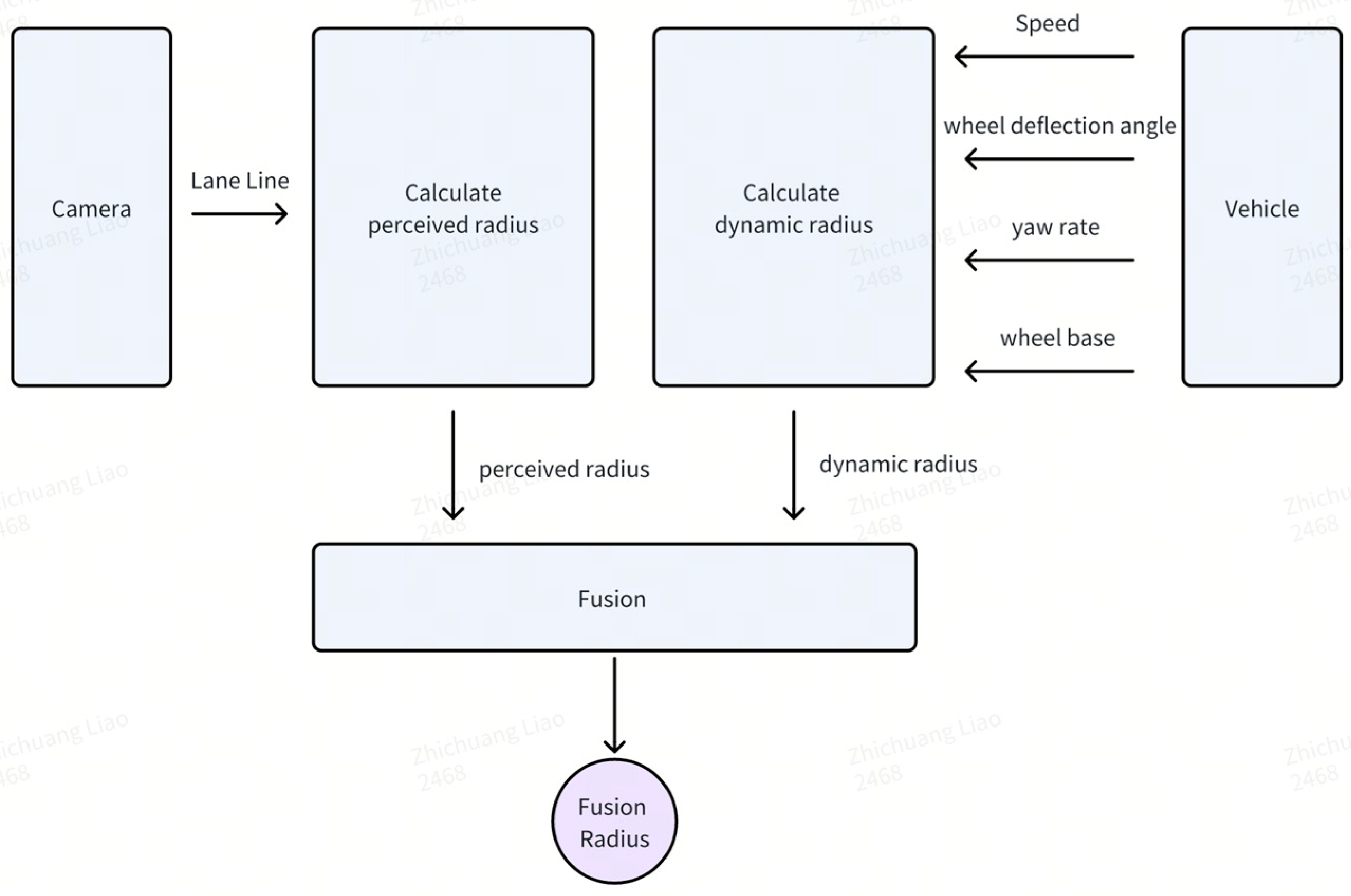
In order to attain a better deceleration effect in the curve, a reasonable fusion of the vehicle’s dynamic radius and the lane line radius is carried out to achieve a smooth filtering of the fusion radius and ensure the comfort of curve control [13]. The calculation process of the estimated fusion radius is shown in Figure 1.
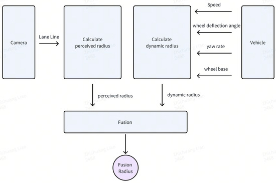
Figure 1.
Fusion radius estimation using combined dynamics and camera data.
According to the lane line equation, the perceived radius of the lane at the pre-viewing position x in front of the vehicle can be obtained as follows:
where and are the first-order derivative and second-order derivative of lateral distance y relative to the vehicle at the pre-viewing position on the lane line. The relationship between x and and is as follows:
In actual vehicle control, as speed increases, a longer preview distance is required to ensure timely deceleration before entering curves. That is, the pre-viewing position in front of the vehicle is related to the current vehicle speed and the pre-viewing time . Considering that the length of the lane line input by perception is limited, the pre-viewing distance should therefore not exceed the valid length of the lane line. Hence, the pre-viewing position of the vehicle is
Based on the above descriptions, according to current vehicle speed and the pre-viewing time t, the pre-viewing position x is calculated through Equation (5); then, by substituting the preview position x into Equations (3) and (4) respectively, the first-order and second-order derivatives of the pre-view position x of the vehicle on the lane line can be obtained; and finally, by substituting the calculated first-order and second-order derivatives into Equation (2), the perceived radius of the road ahead can be obtained.
In actual scenarios, it is common to encounter unclear lane lines and inaccurate perception and recognition of lane lines. If the curve speed limit completely depends on the perception system, then in this case, the function of the curve speed limit will be unavailable. To solve this problem, the vehicle’s own dynamic turning radius and the lane previewing radius are fused together to obtain the curve fusion radius, and this radius is used as the basic radius basis for curve pre-deceleration.
During the driving process of the vehicle, it has a dynamic turning radius itself, and the vehicle’s own turning radius can be calculated using the following formula:
where is the axle spacing of the vehicle, is the wheel deflection angle of the vehicle, and is the yaw rate of the vehicle. is the speed threshold for judging whether the vehicle is at high speed.
In summary, the calculation method of the curve fusion radius is as follows:
where is the radius threshold for the validity of the dynamic radius, and is the weighting coefficient, which takes a value between 0 and 1.
2.3. Filtering Techniques
Both the radius calculated through the lane line and the vehicle’s dynamic radius has significant noise, and this noise has a significant impact on the final speed limit effect. Some noises may cause the vehicle to accelerate and decelerate frequently in the curve, affecting the comfort of the ride. Therefore, some filtering processing needs to be performed on the fusion radius.
The filtering processing of the radius in this paper includes four stages: mean filtering, variable parameter first-order low-pass filtering based on the radius value, variable parameter first-order low-pass filtering based on the error ratio, and variable parameter first-order low-pass filtering based on the radius change characteristic [15,16].
2.3.1. Mean Filtering
In order to effectively avoid sudden changes in the signal and smooth the signal, for the previous frames of the original value of the fusion radius, after eliminating the maximum and minimum values, an average processing is performed to obtain the mean filtering value of the fusion radius. The filtered radius obtained in this stage is denoted as
where Ri represents the original radius value of the curve in the i-th frame, and max{Ri} and min{Ri} represent the maximum and minimum radius values among the N frames.
2.3.2. Variable Parameter First-Order Low-Pass Filtering
When the radius is small, the fluctuation of the radius is large, so when the radius is small, the degree of filtering should be stronger; that is, the filtering coefficient increases with the increase of the mean filtered value of the fusion radius. The filtered radius in this stage is
where f(R1) is an empirical formula related to R1, and is the filtered radius in the last iteration.
2.3.3. Variable Parameter First-Order Low-Pass Filtering Based on Error Ratio
Considering the error ratio in vehicle control, it is necessary to quickly adjust to the correct radius value when significant errors occur to prevent excessive distortions that can impair vehicle handling. Specifically, a larger error ratio necessitates a larger filtering coefficient to ensure accurate control. The filtered radius obtained in this stage is
where is the filtered radius in the last iteration, andthe calculation method of the error ratio is
2.3.4. Variable Parameter First-Order Low-Pass Filtering Based on Radius Change Characteristics
If the filtered radius error is greater than the limit, it is considered a large radius error condition, and a larger filtering coefficient is used to quickly follow the radius to avoid the problem of slow acceleration after exiting the curve. The filtered radius obtained in this stage is denoted as ; that is,
where the radius error is
In the above filtering process,, , and are all empirical formulas, and their values are all between 0 and 1. , , and represent the values of the corresponding radius in the last iteration. The final lane radius input to the bend control module is denoted as .
3. Curve Cruise Control with Integrated Speed Regulation
The curve cruise speed control module is designed to regulate the vehicle’s speed while navigating through a curve. The current longitudinal acceleration of the vehicle should be reduced according to the lateral acceleration of the vehicle after entering the curve, with the aim of ensuring that there will be no uncomfortable sudden acceleration or deceleration in the scene of curve cruising and also ensuring that the vehicle speed is not too fast when entering the curve. The curve cruise control module should ensure that the vehicle is in a stable state when driving in the curve. Therefore, when the preceding vehicle is cruising in a curve (with a fixed curvature), the vehicle should follow the preceding vehicle with a stable time gap.
The curve cruise speed control in this paper is shown in Figure 2 and it involves several key steps. First, curves are categorized into different levels, with each level assigned a specific maximum speed limit. Second, hysteresis zones are defined for each level of curve to enhance speed control stability. Next, the level of the current curve and its corresponding maximum speed limit are determined based on the calculated fusion radius. Finally, the vehicle’s speed is regulated according to this predetermined speed limit. Detailed explanations of each step are provided in the following sections.

Figure 2.
Curve cruise control.
3.1. Speed Limit Hysteresis Zones
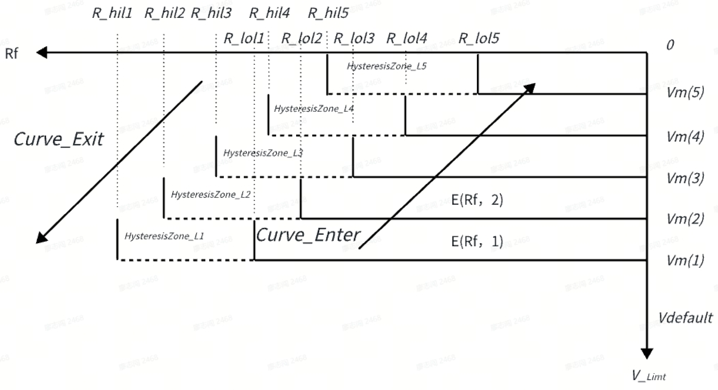
The curve radius may change due to the different stages of the vehicle in the curve or the different parts of the perceived curve [17]. To solve the problem of speed limit oscillation caused by the frequent changes in the radius within the curve, a curve speed limit hysteresis zone is established. The curve speed limit hysteresis zone is used to determine whether the vehicle needs to be speed-limited and how high the speed limit is. The curve speed limit hysteresis zone is shown in Figure 3.

Figure 3.
Hysteresis zone.
Whether the vehicle needs to be speed-limited near this hysteresis zone is determined by the actual radius :
That is, the speed limit strategy for the vehicle near this hysteresis zone is as follows. If the output of is 1, it indicates that the vehicle needs to limit the speed; if the output of is 0, it indicates that the vehicle does not need to limit the speed. refers to the speed limit state of the previous control. That is, when the curve radius is less than the entering speed limit radius thresholds , the vehicle is speed-limited; when the curve radius is greater than the exiting speed limit radius threshold , the speed limit is lifted; and when the curve radius is between the exiting speed limit radius threshold and the entering speed limit radius threshold , the speed limit state remains the same as that of the previous control cycle.
3.2. Speed Limit Grading
The curves in actual roads are not fixed values. Even for the same curve, during the process from entering the curve to exiting the curve, the road curvature changes from small to large and then from large to small. This requires the vehicle to have different speed limit capabilities for different curves or has different adaptive speed limit capabilities for different stages of the same curve; that is, the speed limit is higher for curves with larger radii and lower for curves with smaller radii. To solve this problem, the curves are classified according to the curve radius, and the maximum speed limit for different levels of curves is different.
The maximum speed limit for the curve can be expressed by the following formula:
where is the enable-value of the speed limit for the -th level curve, is the maximum speed limit value for the -th level curve, is the set maximum speed limit level, and is the set maximum speed of the vehicle.
If , it indicates that when the speed limit of the highest-level curve is activated, the maximum speed limit at this time is the speed limit value , corresponding to the highest-level curve. If the speed limit of the (i + 1)th level curve is not activated but the speed limit of the ith level curve is activated ( and ), then the maximum speed limit is the speed limit , corresponding to the i-th level curve. If none of the curves of all levels are activated (), then the speed limit value for curves is the set maximum speed . As shown in Figure 4, the curve radius is divided into five levels. Each level corresponds to a hysteresis zone and a speed limit value. The higher the grade, the lower the speed limit value ( > > > ), and the higher the grade, the lower the entry radius and exit radius ( > > > > ; > > > > ).
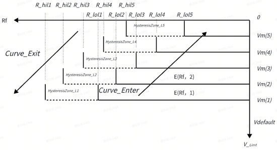
Figure 4.
Speed limit grading.
For the dataset {}, we can obtain a basic value based on . At various vehicle speed , engineers can obtain the range of R by passing the curve with the maximum lateral acceleration. To avoid too frequent control adjustments due to the measurement fluctuations of the lane radius, we add hysteresis for R at various speed limit values.
As shown in Figure 4, the curve radius is divided into five levels. This can achieve the following effects: When the vehicle is entering the curve, as the curve radius gradually decreases, the maximum speed limit of the vehicle will gradually decrease; and when the vehicle is exiting the curve, as the curve radius gradually increases, the maximum speed limit will gradually increase.
The specific rules are as follows. When the curve radius is less than , the maximum speed limit for the curve is ; before the curve radius increases to , this speed limit is maintained; and when the curve radius is greater than , this speed limit becomes invalid. When the previous speed limit value becomes invalid and the curve radius is less than , the maximum speed limit for the curve is ; before the curve radius increases to , this speed limit is maintained; and when the curve radius is greater than , this speed limit becomes invalid. When the previous speed limit value becomes invalid and the curve radius is less than , the maximum speed limit for the curve is ; before the curve radius increases to , this speed limit is maintained; and when the curve radius is greater than , this speed limit becomes invalid. When the previous speed limit value becomes invalid and the curve radius is less than , the maximum speed limit for the curve is ; before the curve radius increases to , this speed limit is maintained; and when the curve radius is greater than , this speed limit becomes invalid. When the previous speed limit value becomes invalid and the curve radius is less than , the maximum speed limit for the curve is ; before the curve radius increases to , this speed limit is maintained; and when the curve radius is greater than , this speed limit becomes invalid. When the previous speed limit value becomes invalid, the curve is no longer speed-limited; that is, the maximum speed limit for the curve is the set maximum speed of the vehicle.
3.3. Speed Limit Control
According to the curve radius and the above formula, the current maximum speed limit for the vehicle can be obtained. When the set cruise speed of the vehicle is greater than the maximum speed limit for the curve or the vehicle speed is greater than the maximum speed limit for the curve, the curve speed limit function is activated. PID is used to control the curve speed, and the calculation method of the requested deceleration is as follows:
where is the proportional control coefficient, is the integral control system, and is the control period.
4. Experimental Data and Analysis
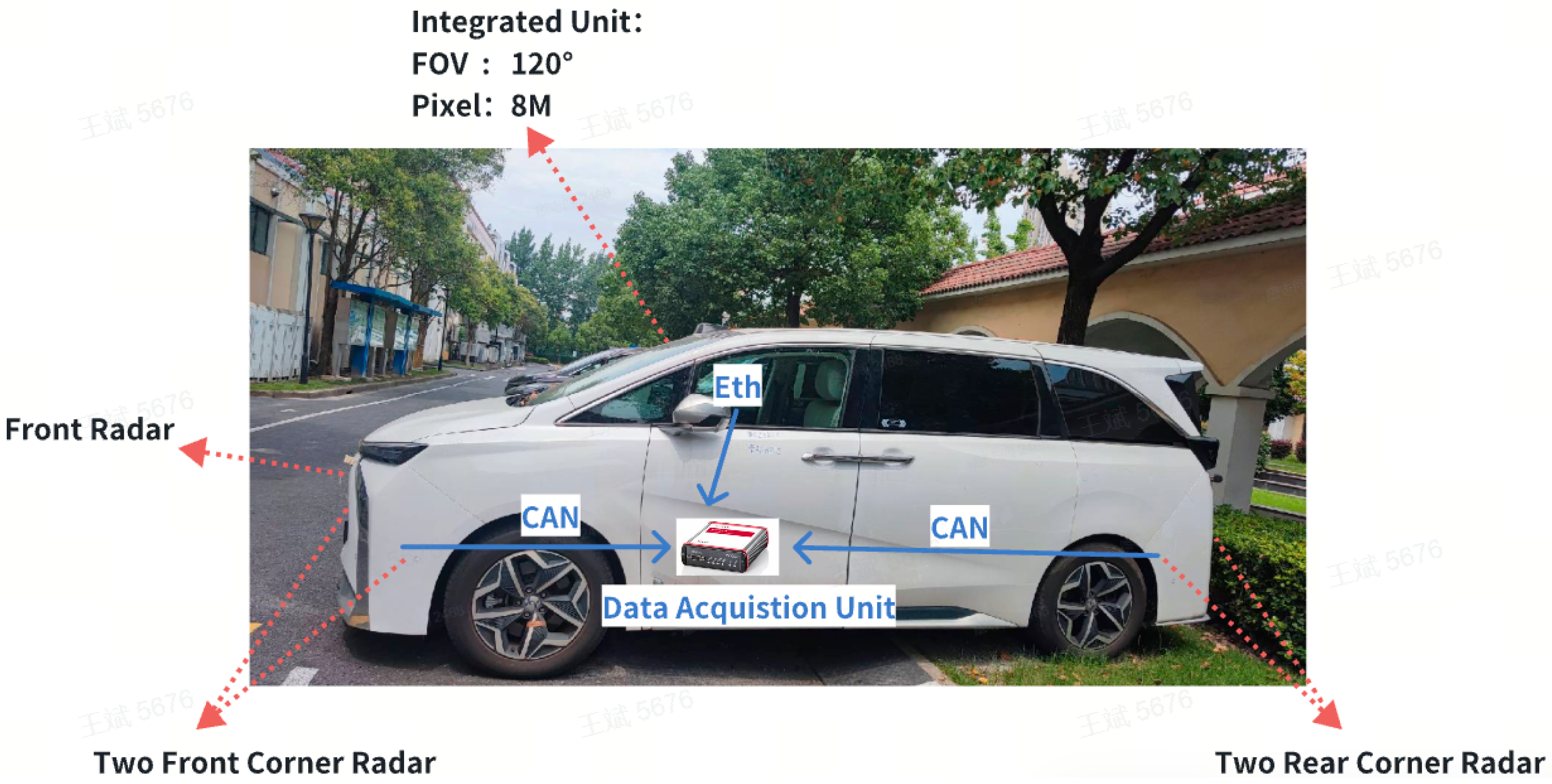
The experimental vehicle is shown in Figure 5. A sensor configuration of 5R1V (one front-view camera, one main radar, two front-corner radars, and two rear-corner radars) is adopted. The FOV of the integrated unit is 120°, with a pixel count of 8 million. During the test, data collection is performed using VX1000(Vector Company, Shanghai, China). Communication between the camera and VX1000 is via ethernet, and communication between the corner radars and VX1000 is via CAN.

Figure 5.
Experimental vehicle.
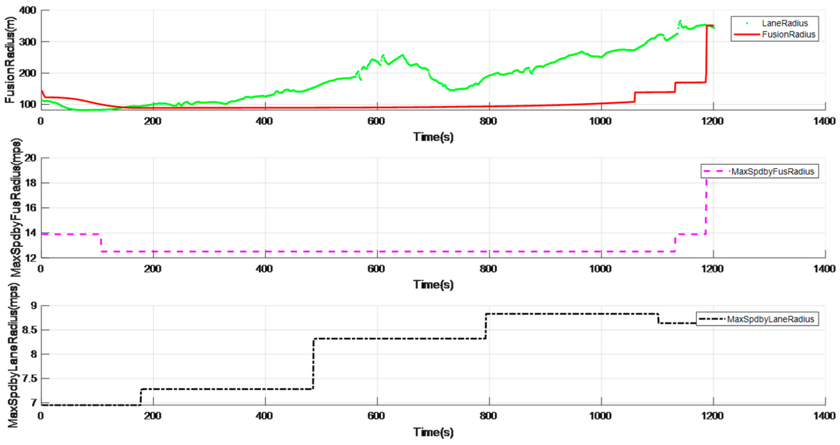
The data collected through this experimental vehicle are analyzed as follows. As shown in Figure 6, the green dotted line is the lane radius calculated through the lane line, and the red solid line represents the fused radius after filtering processing. The pink dashed line represents the maximum vehicle speed obtained through the filtered fused radius, and the black dash-dotted line represents the maximum speed in the curve obtained through the pre-filtered fused radius. From Figure 6, it can be analyzed that the maximum fluctuation of the curve radius before filtering reaches 45 m, and the maximum speed limit in the curve obtained through this fused radius oscillates more frequently, which will cause the phenomenon of deceleration first and then acceleration in the curve; while the curve radius after filtering is relatively smooth, and the maximum speed limit in the curve obtained through this fused radius is stable and reliable.

Figure 6.
Comparison of curve filtering effects.
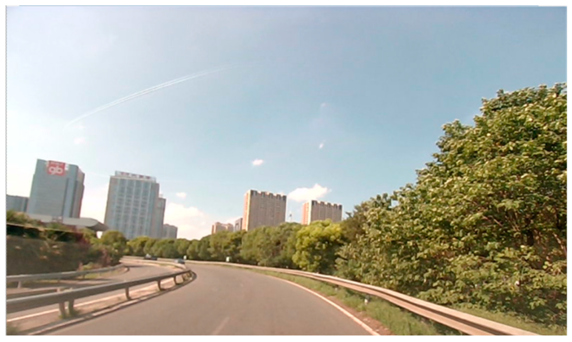
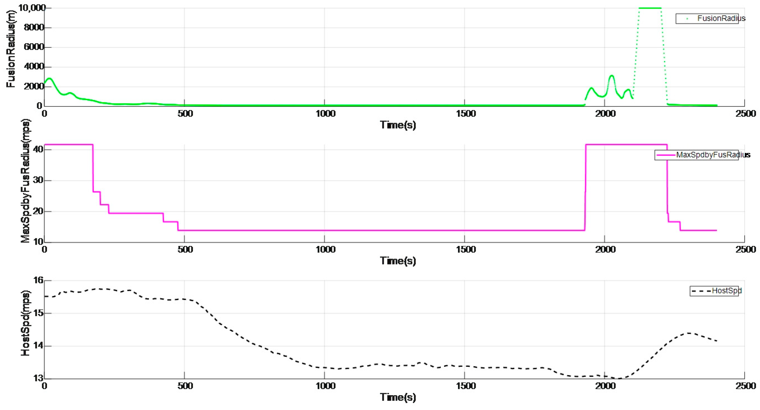
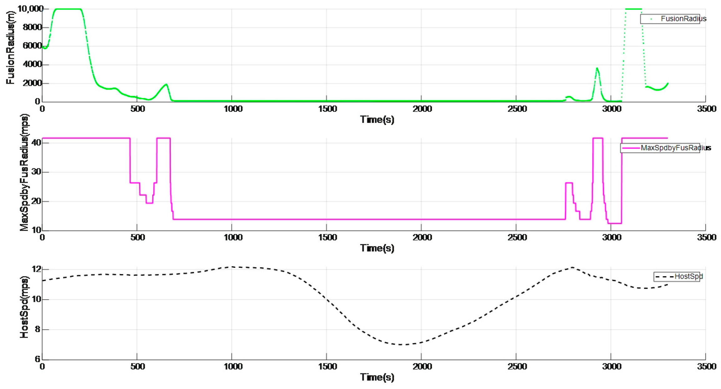
Taking the ramp shown in Figure 7 as an example, Figure 8 shows a complete process of entering and exiting the ramp. In Figure 8, the green dotted line represents the radius of the curve, the pink solid line represents the highest speed limit value of the curve, and the black dashed line represents the actual speed of the vehicle itself, with the horizontal axis all representing time. The vehicle speed before entering the curve is 15.73 m/s, and the lowest speed after entering the curve drops to 13.4 m/s, and the smallest curve radius is 102.7 m. When exiting the curve, the curve speed limit is adjusted to the default value of 41.667 m/s (that is, the curve speed limit is cancelled), and then the vehicle speed increases rapidly. It can be seen that the maximum speed of the curve gradually decreases when entering the curve, and the vehicle speed also decreases accordingly. When exiting the curve, the maximum speed limit of the curve gradually increases, and the vehicle speed also increases accordingly.
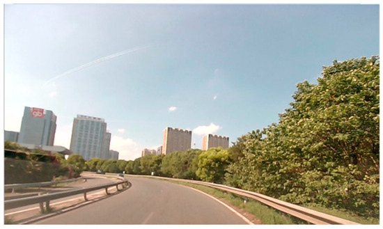
Figure 7.
High-speed ramp.
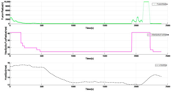
Figure 8.
Complete process of entering and exiting the ramp.
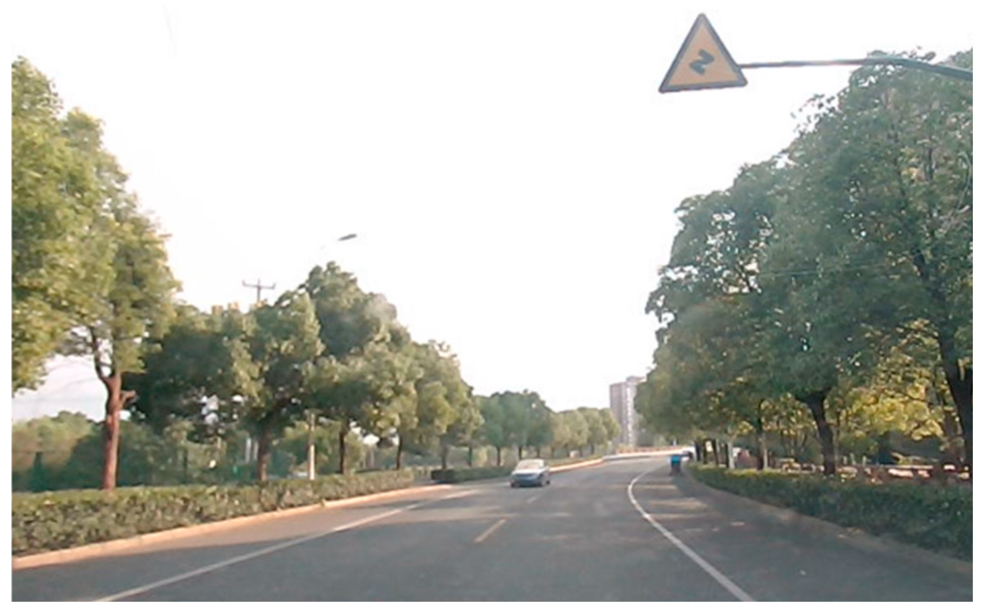
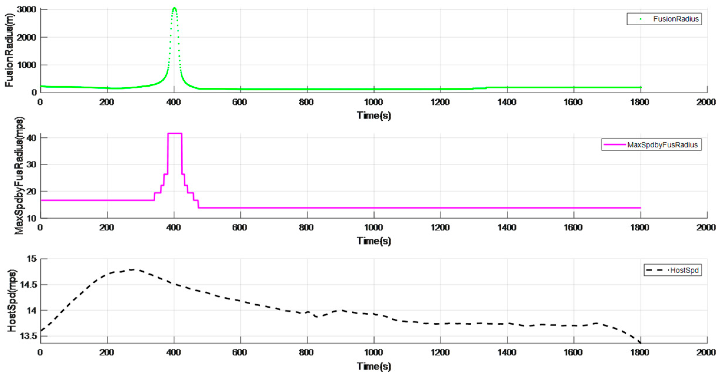
Taking an urban curve shown in Figure 9 as an example, Figure 10 shows the speed limit effect. The minimum radius of this curve is 130 m, the vehicle speed is 14.8 m/s when entering the curve, and the vehicle actively decelerates to 13.7 m/s after entering the curve.

Figure 9.
Urban curve.
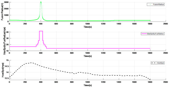
Figure 10.
Speed limit effect of urban curve.
As shown in Figure 11, in the following scenario, the lane lines ahead are not very clear. However, as shown in Figure 12, through the fusion method of the dynamic radius of the vehicle itself and the lane lines, the curve radius can still be calculated as 138.2 m, thereby limiting the maximum speed of the vehicle to 13.9 m/s, achieving the effect of active speed limit on the curve.
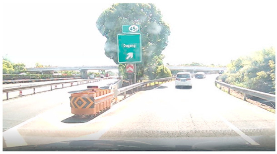
Figure 11.
Curve with unclear lane lines.
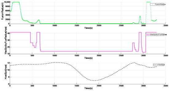
Figure 12.
Speed limit effect when lane lines are unclear.
5. Conclusions
The proposed curve-passing control approach effectively ensures the stability and comfort of autonomous vehicles during high-speed cornering. In particular, the integrated curve radius fusion method proposed in this paper fuses the vehicle’s dynamic turning radius and the lane previewing radius, enabling effective speed control even in scenarios where lane markings are absent or unclear. The multi-stage cascade of filtering methods for the curve radius significantly reduces the noise of the perception data and increases the anti-interference of the curve radius estimation, thereby improving the vehicle’s smoothness and stability during driving. Additionally, the introduction of a curve speed limit hysteresis zone addresses the issue of frequent speed limit fluctuations caused by the chattering of the radius within curved roads. Furthermore, this paper classifies curves into seven types, with speed limits ranging from a minimum of 35 km/h to a maximum of 80 km/h. For example, when navigating a curve with a radius of 150 m, the maximum deviation in the perceived curve radius can reach up to 45 m. If this unprocessed radius data were directly applied for curve control, the vehicle would accelerate from 50 km/h to 60 km/h and then decelerate back to 50 km/h within the curve, resulting in noticeable discomfort for passengers. However, after processing through the system presented in this paper, the vehicle’s speed is stably maintained at 50 km/h upon entering the curve, thereby avoiding the issue of repeated acceleration and deceleration. This system allows the vehicle to implement differentiated speed limit strategies for various curve types and achieve adaptive speed limits at different stages of the same curve. This comprehensive approach enhances the vehicle’s capability to maintain safe and efficient speeds under diverse driving conditions.
Author Contributions
Conceptualization, B.W.; methodology, B.W.; software, Z.L.; validation, S.G. and Z.L.; formal analysis, Z.L.; investigation, B.W. and Z.L.; resources, S.G.; data curation, Z.L.; writing—original draft preparation, B.W. and Z.L.; writing—review and editing, S.G.; visualization, S.G.; supervision, B.W.; project administration, B.W. All authors have read and agreed to the published version of the manuscript.
Funding
This research received no external funding.
Data Availability Statement
The original contributions presented in the study are included in the article, further inquiries can be directed to the corresponding author.
Conflicts of Interest
Authors Bin Wang and Zhichuang Liao were employed by the company Shanghai Baolong Automotive Corporation. The remaining authors declare that the research was conducted in the absence of any commercial or financial relationships that could be construed as a potential conflict of interest.
References
- Xilong, Z. Research on the Development Status of Vehicle Adaptive Cruise Control System. Automob. Appl. Technol. 2024, 49, 29–34. [Google Scholar]
- Ruitian, L. Research on Adaptive Cruise Control Method for Intelligent Vehicles in Curves; Dalian University of Technology: Dalian, China, 2022. [Google Scholar]
- Allaby, P.; Hellinga, B.; Bullock, M. Variable Speed Limits: Safety and Operational Impacts of a Candidate Control Strategy for Freeway Applications. IEEE Trans. Intell. Transp. Syst. 2007, 8, 671–680. [Google Scholar] [CrossRef]
- Baochneg, T.; Tian, L.; Bo, L. Curve Control Technology on Unmanned Vehicle. Comput. Digit. Eng. 2016, 44, 591–595. [Google Scholar]
- Haifeng, L.; Xianzhong, C.; Zhigang, D. Safe Vehicular Velocity Analysis on Express Canale M. Personalization of ACC stop and go task based on human driver behaviour analysis. IFAC Proc. Vol. 2002, 35, 357–362. [Google Scholar]
- Dengke, T. Research on the Relationship between Drivers’ Physiological and Psychological Reactions and Road Alignment; Southeast University: Nanjing, China, 2006. [Google Scholar]
- Gonzalez, D.; Perez, J.; Milanes, V.; Nashashibi, F. A Review of Motion Planning Techniques for Automated Vehicles. IEEE Trans. Intell. Transp. Syst. 2016, 17, 1135–1145. [Google Scholar] [CrossRef]
- Elbanhawi, M.; Simic, M. Sampling-based robot motion planning: A review. IEEE Access 2014, 2, 56–77. [Google Scholar] [CrossRef]
- Min, Z. Research on Fuel Economy of Automatic Variable Speed Vehicle Driving on Ramp; Beijing Institute of Technology: Beijing, China, 2016. [Google Scholar]
- Jiawei, Y. Research on Curve Speed Planning and Trajectory Tracking Control of Autonomous Vehicle; Nanjing University of Aeronautics and Astronautics: Nanjing, China, 2022. [Google Scholar]
- Asadi, B.; Vahidi, A. Predictive Cruise Control: Utilizing Upcoming Traffic Signal Information for Improving Fuel Economy and Reducing Trip Time. IEEE Trans. Control. Syst. Technol. 2011, 19, 707–714. [Google Scholar] [CrossRef]
- Yi, K.; Ryu, N.; Yoon, H.J.; Huh, K.; Cho, D.; Moon, I. Implementation and vehicle tests of a vehicle stop-and-go cruise control system. Proc. Inst. Mech. Eng. Part D J. Automob. Eng. 2002, 216, 537–544. [Google Scholar] [CrossRef]
- Gerdes, J.C.; Hedrick, J.K. Vehicle speed and spacing control via coordinated throttle and brake actuation. Control. Eng. Pract. 1997, 5, 1607–1614. [Google Scholar] [CrossRef]
- Wang, J.; Longoria, R.G. Effect of Computational Delay on the Performance of a Hybrid Adaptive Cruise Control System. In Proceedings of the SAE 2006 World Congress & Exhibition, Detroit, MI, USA, 3–6 April 2006; SAE Technical Papers. Volume 14, pp. 53–57. [Google Scholar]
- Winner, H.; Hakuli, S.; Lotz, F.; Singer, C. Handbook of Driver Assistance Systems; Springer: Berlin/Heidelberg, Germany, 2015. [Google Scholar] [CrossRef]
- Min, D.; Lin, Z.; Yin, Z. Attitude Estimation Method for Quadrotor UAVs Based on Extended Kalman Filter. Mod. Inf. Technol. 2022, 4–7. [Google Scholar]
- Yan, W. Research on Safety and Speed-limit of Oversize Vehicles on Expressway Curve Sections. Highway 2015, 4, 162–168. [Google Scholar]
Disclaimer/Publisher’s Note: The statements, opinions and data contained in all publications are solely those of the individual author(s) and contributor(s) and not of MDPI and/or the editor(s). MDPI and/or the editor(s) disclaim responsibility for any injury to people or property resulting from any ideas, methods, instructions or products referred to in the content. |
© 2024 by the authors. Licensee MDPI, Basel, Switzerland. This article is an open access article distributed under the terms and conditions of the Creative Commons Attribution (CC BY) license (https://creativecommons.org/licenses/by/4.0/).

