Abstract
In the realm of autonomous driving, ensuring a secure halt is imperative across diverse scenarios, ranging from routine stops at traffic lights to critical situations involving detected system boundaries of crucial modules. This article presents a novel methodology for swiftly calculating safe stop trajectories. We utilize a clustering method to categorize lane shapes to assign encountered traffic situations at runtime to a set of precomputed resources. Among these resources, there are precalculated halt trajectories along representative lane centers that serve as parametrizations of the optimal control problem. At runtime, the current road settings are identified, and the respective precomputed trajectory is selected and then adjusted to fit the present situation. Here, the perceived lane center is considered a change in the parameters of the optimal control problem. Thus, techniques based on parametric sensitivity analysis can be employed, such as the low-cost feasibility correction. This approach covers a substantial number of lane shapes and exhibits a similar solution quality as a re-optimization to generate a trajectory while demanding only a fraction of the computation time.
1. Introduction
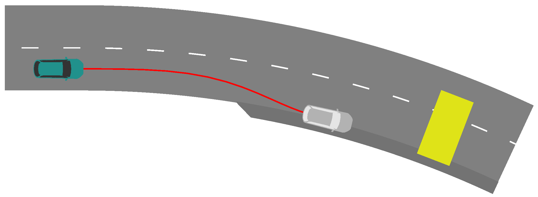
Self-driving vehicles on the road operate in highly complex environments. Their underlying algorithms must cope with a myriad of traffic situations while ensuring route progression and road safety. However, these mathematical algorithms typically act on certain assumptions and expect inputs of a fixed format, narrowing down the means to represent all facets of an encountered real-world scenario and posing substantial limiting factors. Beyond those boundaries, it may not be possible to reliably generate outputs for navigation. In addition, hardware and software flaws are generally unavoidable. Considering these events of potentially undefined or ambiguous behavior, a module that ensures a secure and seamless halt at a safe position is a valuable asset in an advanced driver-assistance system. It is also required by German law for an autonomous car to be able to halt in a safe state in critical situations [1]. Moreover, routine stops at traffic lights or in sight of road blockades, as displayed in Figure 1, are potential use cases for halt trajectories. This paper presents an algorithm for planning such maneuvers.

Figure 1.
Exemplary scenario that may require a stopping maneuver. The yellow obstacle obstructs the street. The turquoise car depicts the initial position; the gray car depicts the final position. The computed safe stop trajectory is displayed in red.
1.1. Classification in Existing Approaches
Traditionally, a software framework for autonomous vehicles consists of several modules processing user and multi-sensor data input, making tactical decisions and translating maneuvers to commands for the actuating elements of the vehicle. In [2,3], a general overview of state-of-the-art research on autonomous driving is given. An essential aspect of navigation is motion and trajectory planning. Therefore, the goal is to find states and controls subject to a time horizon of a few seconds that specify the behavior of the car advancing toward its destination. A survey of different trajectory planning methods can be found in [4,5,6]. Several approaches to compute trajectories exist that originate from graph and optimal control theory or other fields. In this work, we follow an optimization-based approach to generate a trajectory by discretizing an optimal control problem and solving the resulting nonlinear program. The advantage of this method is that different objectives can be effectively integrated into the cost functional or path constraints. Thus, in this approach, accounting for different traffic lanes and the vehicle’s deviation from a reference curve like the lane center can be easily considered and penalized [7,8,9]. Furthermore, the resulting trajectory is (locally) optimal with respect to the defined objective function. However, a good initial guess is typically needed for a solver to converge [7,10]. In the context of autonomous driving, there are strict requirements on robustness and real-time capabilities. There exist approaches to formulate convex problems for trajectory computations to overcome adversity posed by nonlinearity [9,11,12]. These procedures typically feature remarkable convergence performance but heavily restrict the problem formulation as all involved functions have to be convex.
Several fallback solutions have been implemented in the area of trajectory planning. In [13], an approach is presented repairing infeasible trajectories. Collision avoidance trajectory planning in [14,15] aims to mitigate a crash or lower its severity when a collision is hardly avoidable. In such maneuvers, driving comfort is secondary, and the planned trajectory is close to the limits of what is physically possible.
The goal of our work is to rapidly compute safe stop trajectories with a high degree of driving comfort, assuming an early hazard awareness is given. Although, in general, the standard trajectory planning module is able to generate them, it is highly recommended to develop methods tailored to the motivated use cases. In this manner, the algorithms can have a lower computation time, feature better solution quality, and pursue a different approach, leading to a lower probability of failing or generating unfavorable solutions. In a critical situation, the conventional procedure of trajectory planning may have already exhausted the allowed computation time. Thus, the subsequent calculation of the safe stop trajectory must deliver a maneuver immediately to retain a short response time by the autonomous vehicle. If the computation is more resource-intensive, it may be necessary to run it constantly in parallel, even though the outcome of the invested computational effort might never be used. In both successive and concurrent strategies, a low demand for computational resources at runtime is highly advantageous.
In contrast to the great research interest in trajectory planning algorithms, there are only a few publications regarding the planning of safe stop trajectories in particular. Salvado et al. [16] computed safe stop trajectories using a graph-based algorithm employing motion primitives. Wang et al. [17] interpolated grid points with polynomials and selected the one that avoided static obstacles and was feasible with respect to a vehicle dynamics model. An algorithm was subsequently utilized to calculate a velocity profile, avoiding dynamic obstacles. Svensson et al. [18] pursued a two-phase methodology. During a precomputation phase, optimal control problems for several endpoints were solved offline, and the resulting trajectories were stored for later use. During runtime on an autonomous vehicle, the environment was subdivided into regions, indicating how favorable it was to stop in the respective areas. Upon this, the best endpoint for the present situation was selected, which corresponded to a precomputed trajectory. However, their algorithm is restricted to straight roads.
1.2. Contributions
In our work, we advance the methodology initially established by Svensson et al. [18] and others in the domain of trajectory planning, specifically focusing on the area of safe stop strategies. Our approach is distinguished by a two-pronged contribution. Firstly, we extend previous efforts in [18] by incorporating advanced clustering and optimization techniques to address the challenge of navigating arbitrary road shapes. This is achieved while ensuring real-time capabilities through the use of parametric sensitivity analysis, allowing for the dynamic adaptation of precomputed trajectories to current conditions. This not only ensures a near-optimal trajectory but also enhances safety and comfort through the smoothness of states and controls.
Secondly, we delve into the realm of nonlinear optimization, a field known for its complexity, especially when applied to time-sensitive tasks. By applying feasibility correction [19]—a method previously explored in contexts for simpler applications [20] and emergency trajectory planning [14]—we introduce a novel perspective to the challenge of trajectory planning, which is now compounded by several non-trivial disturbances that enter the problem in a nonlinear fashion. This approach, utilizing the feasibility correction method as an exemplar of numerical real-time optimization techniques, represents a significant advancement in our capability to dynamically reduce computational complexity in the face of intricate, higher-dimensional disturbances.
1.3. Outline
The remainder of this paper is organized as follows. Fundamental to this work are techniques of parametric sensitivity analysis, depicted in Section 2. In Section 3, the determination of relevant static traffic situations defined through lane centers is described. Upon this, Section 4 reports the process of trajectory computation. The performance of the algorithm is evaluated in Section 5. Finally, Section 6 draws a conclusion about the observed results.
2. Nonlinear Optimization and Parametric Sensitivity Analysis
This section outlines the fundamentals of nonlinear optimization and parametric sensitivity analysis, concluding with a feasibility correction method. The techniques described are later used to solve a discretized optimal control problem, resulting in a trajectory. For further explanations on nonlinear optimization, we refer to [21]. We utilize parameter-dependent nonlinear programs, which allow for post-optimal parametric sensitivity analysis.
Definition 1
(Parametrized nonlinear program). Assuming a vector of parameters in a parameter space . The task
is called a nonlinear program (NLP). , denotes the objective function, while and , express the equality and inequality constraints for optimization variables , respectively. We postulate that , and h are sufficiently often continuously differentiable. A point is called feasible if and hold.
The Lagrangian function combines the objective with the constraints of NLP as a weighted sum.
Definition 2
(Lagrangian function and multipliers). For NLP, the so-called Lagrangian function is defined as
The vectors λ and μ are called Lagrangian multipliers.
Inequality constraints fulfilled by equality are called active. The corresponding indices form the active set. The other, inactive inequality constraints do not influence the solution of the problem locally.
Definition 3
(Active set). For a feasible point , the set is called an active set.
By this definition, we define a regularity assumption.
Definition 4
(Linear independence constraint qualification (LICQ)). A feasible point satisfies the linear independence constraint qualification (LICQ) if the gradients are linearly independent.
Following this, we can formulate first-order necessary conditions for NLP, the so-called KKT conditions.
Theorem 1
(KKT conditions). Let be a local minimum of NLP fulfilling LICQ (Definition 4). Then, there exist uniquely identified such that
Thereby, the operator diag maps a vector onto a diagonal matrix. A tuple with feasible fulfilling (2) is called a KKT point.
Proof.
Refer to [22] (pp. 195–207). □
An additional characterization of local minima is given by sufficient conditions.
Theorem 2
(Second-order sufficient conditions). Let be a KKT point of NLP complying with LICQ (Definition 4). The critical cone is defined by
Furthermore, let
Then, is a strict local minimum of NLP.
Proof.
Refer to [22] (pp. 207–212). □
Based on the necessary conditions for optimality from Theorem 1, algorithms exist to determine local minima [23]. These entail a relatively high computational effort if F, g, and h are non-convex. However, when treating a large set of similar problems that only differ slightly in their parametrization p, the so-called sensitivity theorem is a powerful tool to exploit. The theorem is based on the implicit function theorem (see [24]) and can be stated as follows.
Theorem 3
(Sensitivity theorem). Let fulfill the second-order sufficient conditions from Theorem 2 for NLP and some nominal parametrization , together with Lagrangian multipliers . Additionally, assume for . Then, there exists a neighborhood of and continuously differentiable functions and , such that for the following properties hold:
- 1.
- .
- 2.
- The active set does not change, i.e., .
- 3.
- fulfills LICQ (Definition 4).
- 4.
- is a local minimum of NLP with Lagrangian multipliers .
Proof.
Refer to [25]. □
Furthermore, the theorem provides the means to determine the sensitivity derivative .
Corollary 1.
A representation of can be obtained by determining the unique solution of the linear equation system
Proof.
This is equivalent to the linear equation system (5). Because of [26], stating the regularity of , there exists exactly one solution. □
The sensitivity derivative can be used for a first-order Taylor approximation of the solution of NLP as
However, such an approximation is not feasible in general, violating the constraints in NLP. Hence, additional steps need to be taken to eliminate the error in the constraints. We showcase the feasibility correction method on a problem with equality constraints. For , consider the problem
The parameter is relevant for the correction of the feasibility error. The derivative specifies how the solution z changes when components of the vector are decreased or increased. It can be computed similarly as the derivative with respect to p. Let and denote the constraint of problem (8). The Lagrangian function of problem (8) is
Let be the nominal parameter and a known solution of the corresponding nonlinear program with related Lagrangian multiplier . Then, for (9), it holds that
where I denotes the identity matrix. By inserting these equations into system (5), we conclude with a calculation rule for . For the approximation , the feasibility error is given by . This error is gradually reduced to zero, leading to an iterative correction. In an iteration , the update step
is performed. As stated by the following theorem, this method converges and the limit has no constraint violation.
Theorem 4
(Convergence of the feasibility correction method). Assume the sensitivity theorem (Theorem 3) holds for a reference solution . For a parametrization , the term is defined as (7), and is defined as (12). Then, there exists a neighborhood of , such that for all , the following holds:
Furthermore, converges to a fixed point.
Proof.
Refer to [19] (pp. 37–46). □
If the change in the parametrization is small, i.e., inside the neighborhood , the sensitivity theorem (Theorem 3) assures that the active set does not change. Hence, for the feasibility correction, active inequality constraints can be considered equality constraints, and inactive constraints can be neglected.
3. Identifying Traffic Situations with Fréchet Clustering
In the further course of this work, we parametrize a nonlinear program NLP with static traffic situations. As seen in the previous section, the parameter difference during the sensitivity update must be sufficiently small. Therefore, we first categorize all possible static traffic situations and compute reference solutions for each category. At runtime, the most similar reference traffic situation is selected, and a feasible stopping maneuver is generated. We introduce a metric to determine different categories to classify and compare static traffic situations. A suitable way of performing this is to look at the difference between two lane centers. For this, we introduce the Fréchet distance.
Definition 5
(Fréchet distance). Let be two polygonal, parametrized curves. Each curve is determined by a set of vertices. We denote the set of all such polygonal curves with . Additionally, let be the set of all continuous, monotonously increasing and surjective functions . Then, the Fréchet distance is defined by
Bringmann et al. presented an efficient algorithm to calculate the Fréchet distance in [27]. Here, the method introduced in [28], which relies on the so-called free-space diagram to determine which point pairs of the two curves have a distance below a given threshold, is essential. Building upon this, Bringmann et al. implemented additional rules to improve performance.
In real-world traffic, we may encounter countless different lane centers. To reduce complexity at runtime, it is necessary to identify representative curves from a data set of lane centers, which we can focus on during a preparation phase. Every element in the data set should be similar or assignable to a representative. We use the k-means-based clustering algorithm developed by Buchin et al. [29] to find such representative curves. The well-known k-means consists of two main components: a function measuring distances and a function calculating a cluster center, which represents a cluster [30]. Buchin et al. employed the Fréchet distance to measure the distance between two elements. To update the mean of a subset of elements, they utilized the parametrization from the Fréchet distance. The computation of the Fréchet distance yields a parametrization of both curves. Hence, for each vertex of the old center, there exists a point with the same parametrization value on every curve in the subset. The center of the smallest enclosing circle of these points represents the vertex of the new center. For sufficiently simple cluster centers, Buchin et al. proposed restricting the number of vertices in a cluster center. We allow up to ten vertices.
For our numerical experiments, we employed a training and evaluation data set. To obtain them, we documented the trajectory of a research vehicle navigating in manual mode within a suburban environment. The vehicle was outfitted with an advanced localization framework, as detailed in [31], ensuring an accurate position estimation. Subsequently, the acquired data were organized into two distinct sets of lane centers. The training data set encompasses 239 curves, while the evaluation data set comprises 105 curves. Both can be found in [32]. The algorithm presented in this paper is configured to aim for good performance with respect to the training data set. Eventually, the evaluation data set was used to assess the performance of the final algorithm. As an estimate for all possible lane centers, we used a training data set of lane centers. Figure 2 shows the results of the clustering on our training data set, where the number of clusters was set to ten.
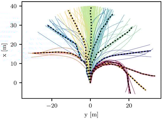
Figure 2.
Clustering results shown on the training data set. Each color depicts one cluster. The computed cluster centers are displayed with a black dotted line.
Each representative lane center originating from the cluster centers represents an individual optimization problem we can solve before runtime. We chose the coordinate values of the vertices as parameters to make use of the sensitivity theorem (Theorem 3) discussed in Section 2. The actual lane center encountered by a driving car was then considered in a re-parametrized problem for which, upon correct classification, we could obtain an immediate approximate solution and an improved one using feasibility correction.
Previously, the lane centers were described by a function mapping the interval to a polygonal curve in , as defined in Definition 5. In the following, we describe a lane center as a flattened set of vertices. Every polygonal curve can be described by both descriptions. However, using the characterization based on vertices makes it easy to compute the translation between two curves, if they follow the standardized form. By linearly interpolating between the vertices and parametrizing the resulting curve, we conclude with a curve as defined in Definition 5. We establish a standardized form of the lane centers to incorporate them in our optimizations in a unified manner.
Definition 6
(Standardized lane center). Let and . An element comprises two-dimensional vertices. We denote as a standardized lane center if it complies with the following properties:
- Adjacent vertices have a fixed distance, i.e.,
- The start point is the origin of the coordinate system, i.e., .
- The first segment has the same orientation as the x-axis, i.e., .
- Two adjacent segments shall have a similar orientation, i.e.,where returns the polar angle of the point .
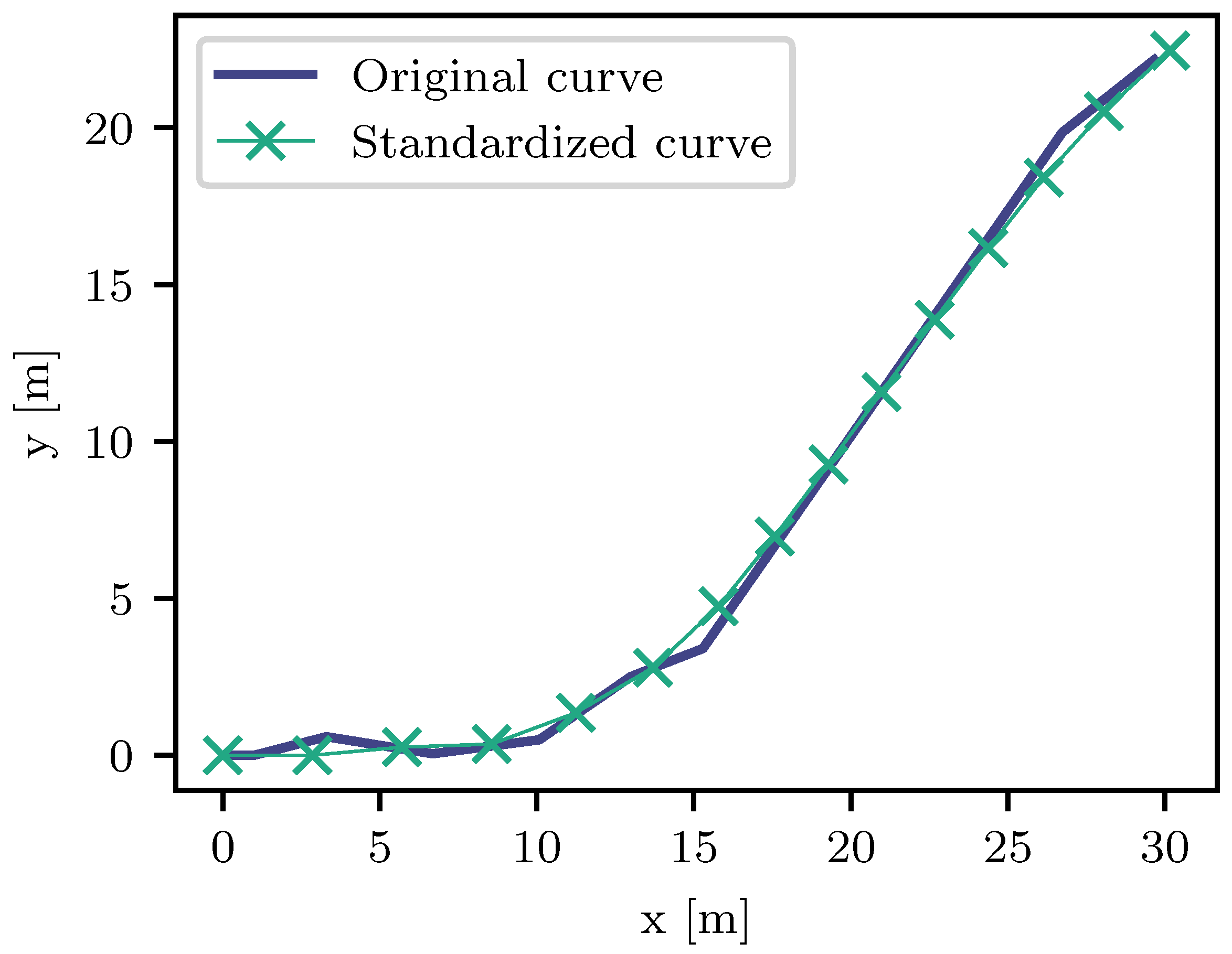
We chose as the fixed number of vertices and as the total length of a lane center, leading to a distance of between two adjacent vertices. It was assumed that the controlled vehicle was initially at the origin of the coordinate system, and its orientation was aligned with the x-axis. Additionally, we assumed that the vehicle’s position corresponded to the start of the lane center, with the same orientation as the first lane center segment. These assumptions decreased the number of cases which had to be considered during trajectory computation. Hence, we required each standardized lane center to meet these requirements. The cluster centers resulting from the above-described clustering algorithm may have kinks, which can cause issues in the trajectory computation algorithm. Thus, in a process of standardization, we performed smoothing by fitting a B-spline curve to the cluster center using the B-Spline calculation method from [33]. Since the first two vertices of the standardized lane center are fixed, the start point of the B-Spline is the second fixed vertex. The B-Spline is then determined to fit the subsequent vertices of the curve that shall be standardized. Beginning with the start point of the B-Spline, the next vertex of the standardized lane center is the point on the B-Spline with the fixed distance to the current one. Figure 3 depicts an example of the standardization process.
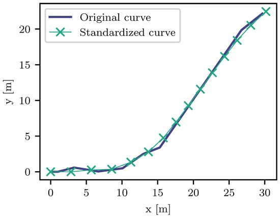
Figure 3.
Process of standardization: The original curve is one of the cluster centers. The resulting standardized curve complies with the described standardized form.
4. Trajectory Computation Methods
Below, we describe our trajectory computation algorithm. First, we outline the optimal control problem, which is transcribed into a nonlinear program. The solution of this problem describes a trajectory. It is parametrized by a standardized lane center from Definition 6. After that, we summarize the precomputation phase, where this problem is solved by a conventional NLP solver for the cluster centers from Section 3. Finally, we depict the runtime phase, where the solution of the problem parametrized by the runtime lane center is approximated. For this, we pursue a selection of a precomputed trajectory and an update based on the techniques from the parametric sensitivity analysis described in Section 2.
4.1. Problem Formulation for Trajectory Computation
In this section, we formulate a problem leading to a safe stop trajectory for a vehicle along a given lane center. In order to generate viable stopping maneuvers for a car, we must consider its kinematics and predict its behavior under certain control inputs.
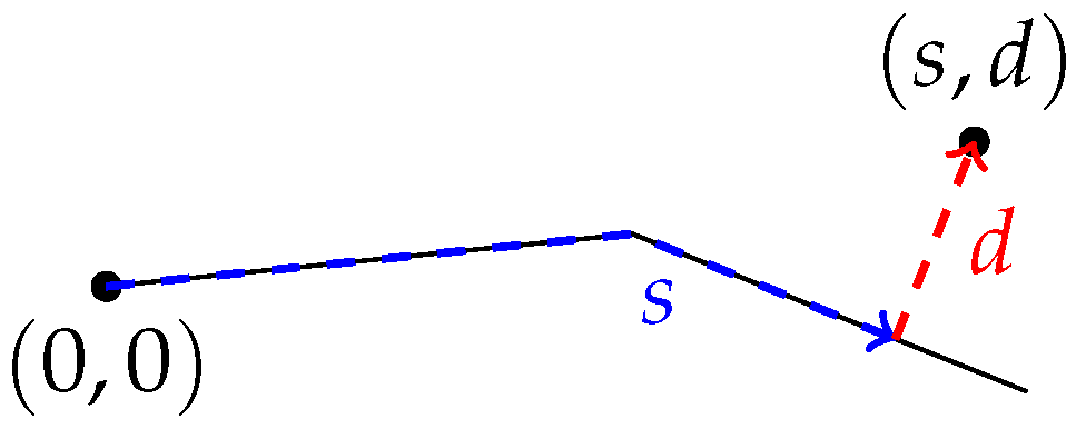
We introduce Frenet coordinates [34] to uniformly define the final positions of a car with regard to any lane center. By means of Frenet coordinates with respect to lane centers, we can specify the final positions uniformly and deduce the designated orientation of a car. A Frenet coordinate pair describes a Cartesian point with respect to a parametrized curve. Here, d quantifies the distance between and the curve, while s describes the length from the start to the point of the curve at the minimum distance, as in Figure 4. Note that d is a signed value depending on whether the given point is on the left (+) or right side (−) of the curve. The function maps Frenet coordinates regarding a curve to the corresponding Cartesian coordinates and the orientation of the curve segment closest to the point. It is defined by the result of Algorithm 1.
| Algorithm 1 Conversion from Frenet to Cartesian coordinates |
Inputs:
|
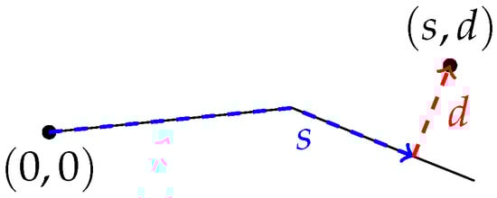
Figure 4.
Exemplary point in Frenet coordinates. The black line describes the lane center.
In the following, we formulate an optimal control problem (OCP) to calculate safe stop trajectories for a given standardized lane center . We set the number of states as and the number of controls as . Assuming a process time interval with , the functions
map the time to six states and two controls, respectively. For ,
- is the position in Cartesian coordinates in
- is the yaw angle in
- is the steering angle in
- is the speed in
- is the acceleration in
- is the steering angle velocity in
- is the jerk in
The optimal control problem is given by
The function in the cost function computes the shortest Euclidean distance between the position and the polygonal line defined by p. The weights are chosen as
The weights are selected to ensure that the resulting trajectory describes a smooth stopping maneuver while keeping the states and controls as far as possible from the bounds of the inequality constraints. This not only enhances the driving comfort but also improves the convergence behavior of the feasibility correction applied at runtime. The vehicle dynamics f are defined by a single track model [35] with additional derivative layers to ensure smooth values for the actuating elements. Hence, f is defined as
We chose the constants to be
based on the research vehicle described in [36]. Thereby, l describes the wheelbase, and the other constants model the physical limitations of the car in normal driving mode. The function maps a given angle by means of modulo operations to the interval . Additionally, we set an initial speed and a final position in Frenet coordinates. The final orientation was established to ensure the vehicle came to a halt parallel to the lane center, which is a preferred alignment to avoid obstructing the entire street.
This OCP was solved using the direct method. Therefore, it was discretized and transcribed into a nonlinear program. For discretization, the time interval was discretized equidistantly at discretization points. Hence, the step size is . At every discrete time point , the states and controls are approximated via
The static optimization variables z of the corresponding nonlinear program consist of all states and controls at every discretization point as well as the end time , i.e., and . This discretization scheme is called full discretization. To discretize the differential equation, we employed the trapezoidal method [37]. Let describe a standardized lane center from Definition 6. We conclude with
Thereby, for
and
This is a nonlinear program in the form of NLP. The inequality constraints are defined by fixed intervals. By introducing the projection operator on those intervals, the inequality constraints can be rewritten as . The inequality constraints (28) only contain simple intervals, which are independent of the problem parametrization p. This separation will be handy in the subsequent sections and is the reason why the actual equality constraints are reformulated as inequality constraints.
4.2. Trajectory Precomputation for Cluster Centers
In this section, we aim to compute trajectories along the representative lane centers of all clusters found using the method described in Section 3. To obtain trajectories, we solve nonlinear program (26), which is a discretization of optimal control problem (21). In our experiments, we set the initial speed to and the final position in Frenet coordinates to and . We chose d to be negative since this corresponded to a stopping position at the edge of the road in right-hand traffic. Hence, for each representative lane center, nine trajectories belonging to different final positions were calculated. Problems belonging to the same lane center were solved consecutively, using the previous solution as an initial guess. If the lane center changed, the initial guess for the position and orientation followed a Dubins path. This path is the shortest curve between a given start and end, taking a minimum turning radius into account [38]. We relied on the implementation [39] to compute such curves and used as an approximation for the minimum turning radius [40]. Since the Dubins path only provides an estimate for the position and yaw, the other values had to be guessed differently. We used a simple guess as we set the velocity to linearly decaying and the other values to 0. To solve nonlinear programs, we used the solver Worhp [41] for this work. Finally, all trajectories and corresponding sensitivity matrices were stored for runtime use.
4.3. Trajectory Computation for Arbitrary Lane Centers at Runtime
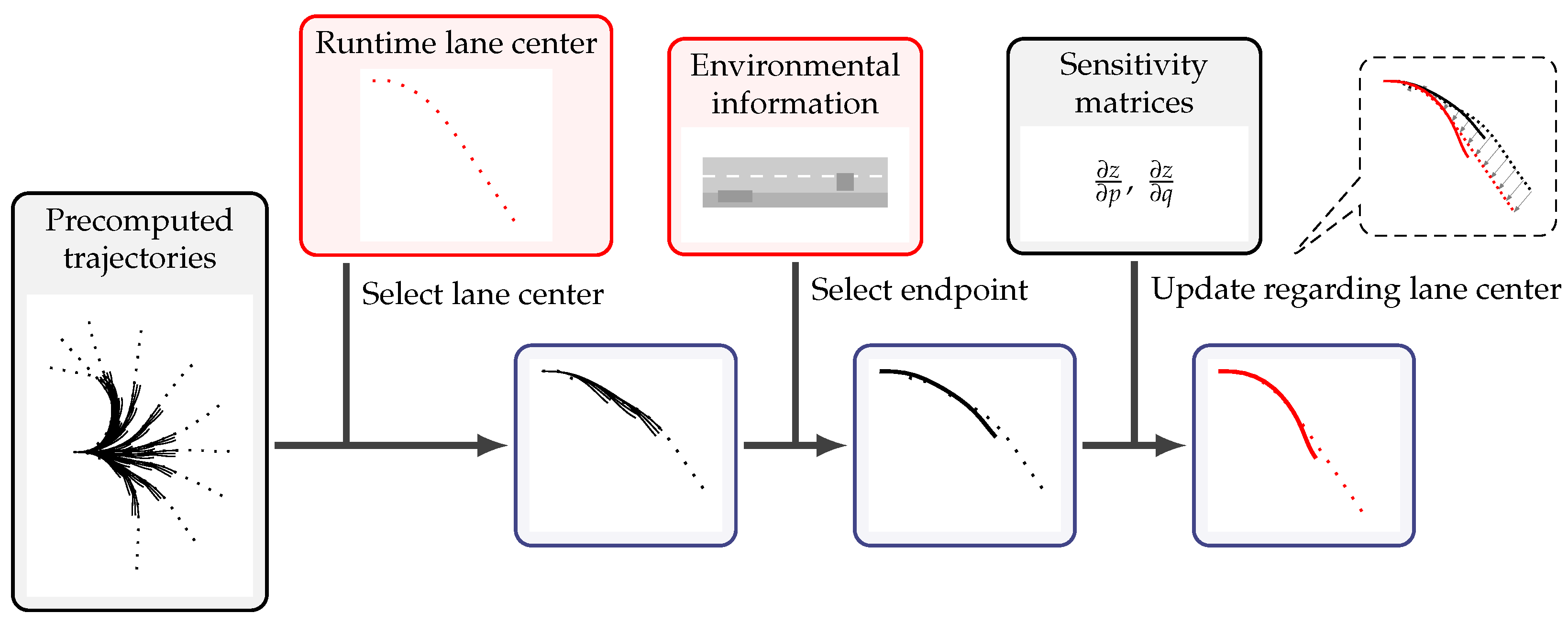
Now, we describe the efficient solution of problem (26) parametrized by the lane center encountered at runtime. Figure 5 gives an overview of our approach to compute a halt maneuver at runtime. First, the static traffic situation had to be categorized, and the respective representative lane center was identified. We applied the Fréchet distance from Definition 5 to find the cluster center that was closest to the lane center encountered at runtime. As a direct consequence of the definition of the Fréchet distance, the Euclidean distance between the endpoints of two lane centers represented a lower bound. Since evaluating the Euclidean norm is considerably faster than computing the Fréchet distance, we suggest listing the representatives in ascending order in terms of the endpoint distance. If the Fréchet distance of an element is smaller than the lower bound of its successor in the list, the search is terminated, and it is assumed that any subsequent elements have a lower Fréchet distance.
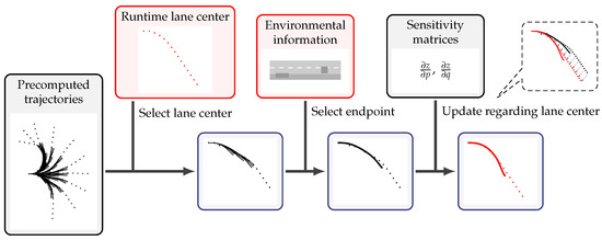
Figure 5.
Process of the trajectory computation at runtime. Gray boxes indicate inputs from the precomputation phase; red boxes indicate inputs from sensor fusion.
For each lane center, there are several precomputed trajectories belonging to different endpoints. Based on the actual information about the environment, a decision has to be made about which halt position the car should reach and which precomputed trajectory should be used. For example, a halt at a side strip is generally preferred over stopping in the center of the lane.
Eventually, the selected trajectory is updated to match the present situation at runtime. We utilized the feasibility correction algorithm from Theorem 4. However, we made minor adaptations. The sensitivity theorem (Theorem 3) states that the set of active inequality constraints does not change in a neighborhood of the reference parametrization. The extent of the neighborhood, though, is generally unknown. Thus, we cannot guarantee that the difference in the parametrization, i.e., the difference between the precomputed and runtime lane center, is small enough. Therefore, in order to be able to obtain a feasible solution, we ensured the fulfillment of the inequality constraints by projecting the solution candidate onto the intervals defining the inequality constraints. Additionally, we tuned the optimal control problem in the precomputation phase so that a precomputed trajectory was as far away from the inequality bounds as possible. In particular, weighting (22) is important. This avoids changes in the set of active inequality constraints at runtime that lead to problems.
We summarize the approach for the trajectory update in Algorithm 2.
| Algorithm 2 Sensitivity-based trajectory computation with feasibility correction |
Inputs:
|
5. Results
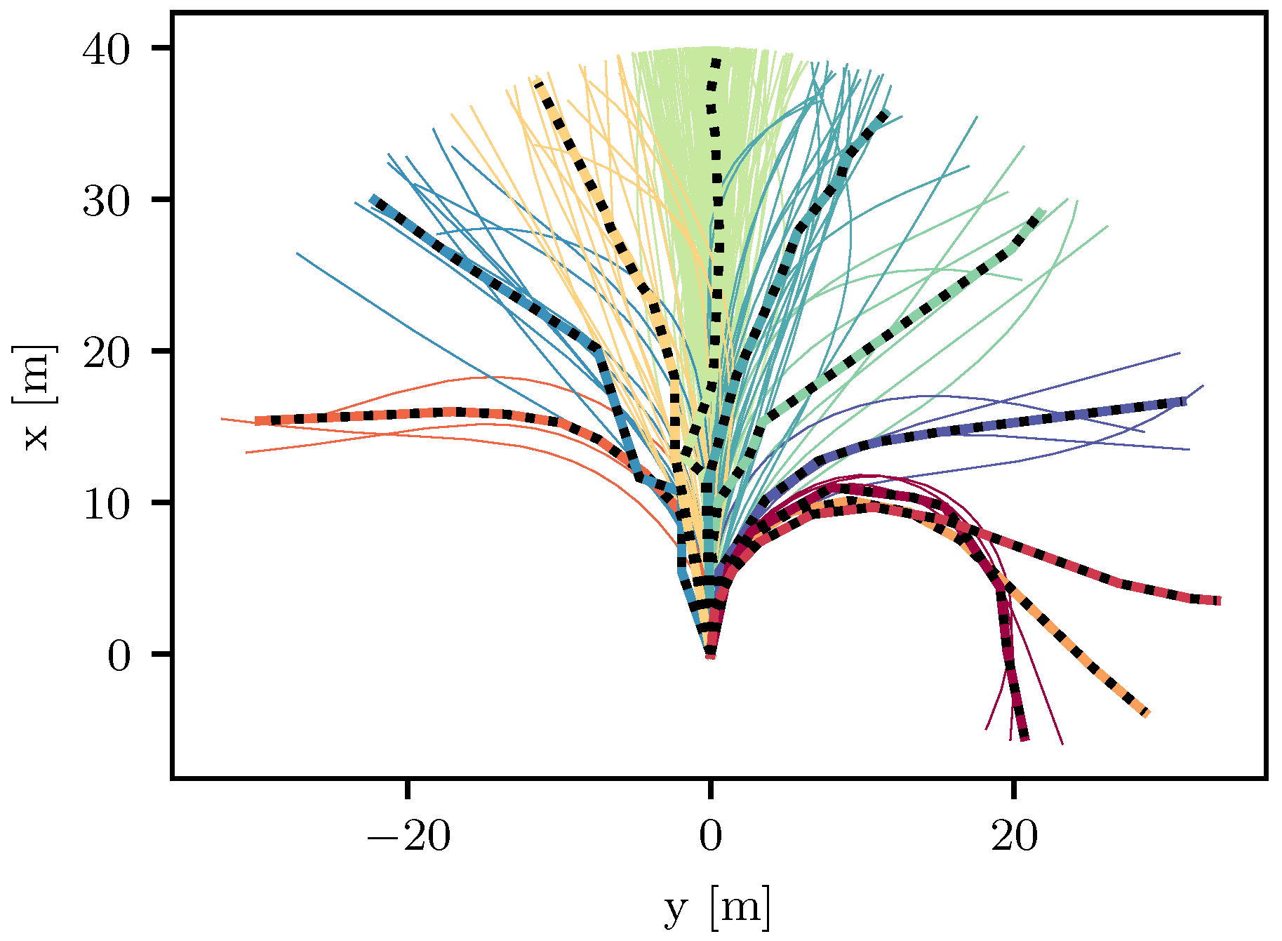
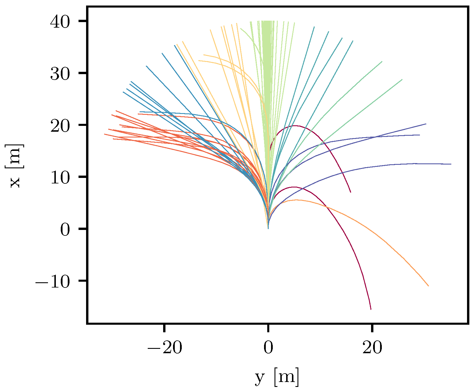
To compute trajectories, we first applied the aforementioned clustering algorithm to the training data set and generated standardized representative lane centers. These were then used to precompute trajectories. In this section, we evaluate our proposed method by applying the runtime algorithm to each lane center in the evaluation data set. These lane centers are converted into the standardized form in Definition 6. The evaluation data set is displayed in Figure 6. The focus of our evaluation is on the utilized feasibility correction algorithm. Hence, we conducted a simulative analysis. We wanted to assess if Algorithm 2 can compute a feasible trajectory for any lane center which may be encountered at runtime. Thereby, the convergence speed was of interest and was evaluated to ensure the proposed method meets the requirements of being ressource-efficient. During the selection process at runtime, we always chose the trajectory with the endpoint in Frenet coordinates. We did not use real-world environmental information for the selection process. Our experiments were conducted on a CPU Ryzen 7 Pro 7840U.
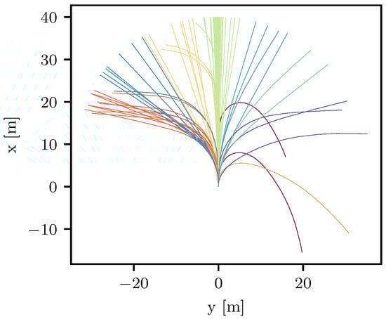
Figure 6.
Evaluation data set with cluster assignment. Each color depicts one cluster.
5.1. Convergence of the Feasibility Correction
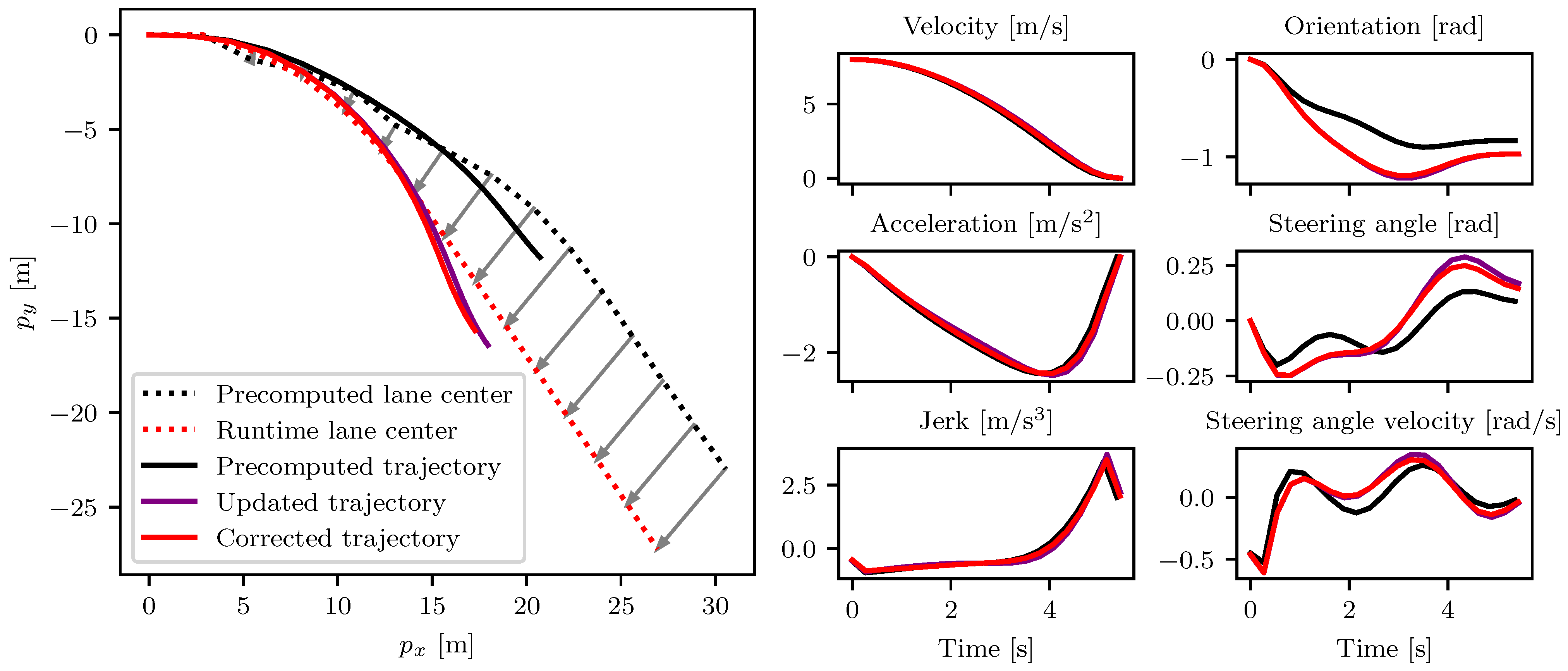
Figure 7 illustrates an example for the trajectory computation algorithm given a specific lane center in the evaluation data set. Here, the trajectory generated by applying the first-order Taylor approximation regarding the lane center (step 2 of Algorithm 2) is already close to being feasible and only shows small deviations from the trajectory obtained after applying further correction steps. Furthermore, it is noticeable that all states and controls are relatively smooth and jump-free. This is a valuable asset for a trajectory planner, as it simplifies the problem for the control module.
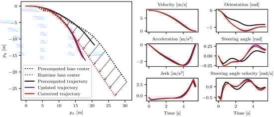
Figure 7.
Exemplary trajectory during the process of trajectory computation. The selected precomputed trajectory, the trajectory after the parametric sensitivity update with respect to changes in the lane center coordinates, and the trajectory after feasibility correction are displayed. On the left, the position in Cartesian coordinates is presented; on the right the other states and controls are presented.
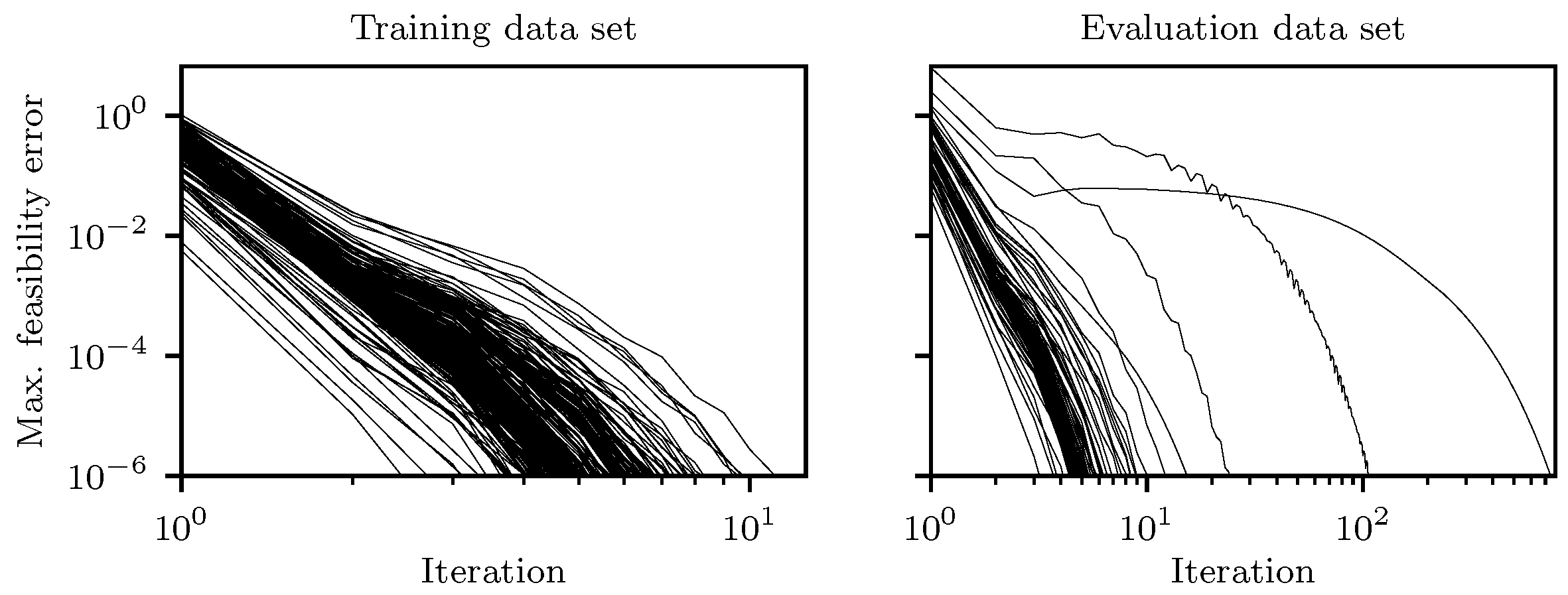
We required a maximum feasibility error of to denote a trajectory as feasible, which was also the requirement during precomputation. When implemented on a vehicle, this tolerance may be relaxed to speed up runtime calculations. Figure 8 displays the course of the maximum feasibility error over the number of iterations for each lane center from the training and evaluation data set. The algorithm exhibits favorable results on both data sets and terminates successfully in all cases. In the evaluation data set, two instances stand out due to their considerably higher convergence iterations compared to others. Specifically, these instances require 105 and 740 iterations to achieve convergence within the prescribed maximum feasibility error. The slower convergence can be attributed to the presence of a sharply curved section in the track recording underlying the evaluation data set. The initial velocity is set to 8, a speed that would be considered excessive for this particular curve in typical traffic conditions. Notably, such sharp curves are absent in the training data, posing a challenge for the algorithm in computing a feasible trajectory within the specified constraints on steering angle and steering angle velocity. At the beginning of the iteration process in the feasibility correction algorithm (Algorithm 2), these constraints are violated by the trajectories resulting from the sensitivity update in steps 2 and 6. The violation is subsequently corrected during projection steps 3 and 7, which introduces an error in the differential equation and counteracts the preceding sensitivity update step. Consequently, many iterations are required to achieve feasibility. Despite these challenges, the algorithm manages to find a feasible solution.

Figure 8.
Feasibility errors in every iteration of the feasibility correction. For each lane center from the training and evaluation data set, one trajectory was computed.
Furthermore, the feasibility correction iteration does not only improve feasibility, but also the objective value. Compared to the trajectory following step 3, prior to the iteration for correcting feasibility errors, the resulting trajectory has an average objective value that is approximately 1% better.
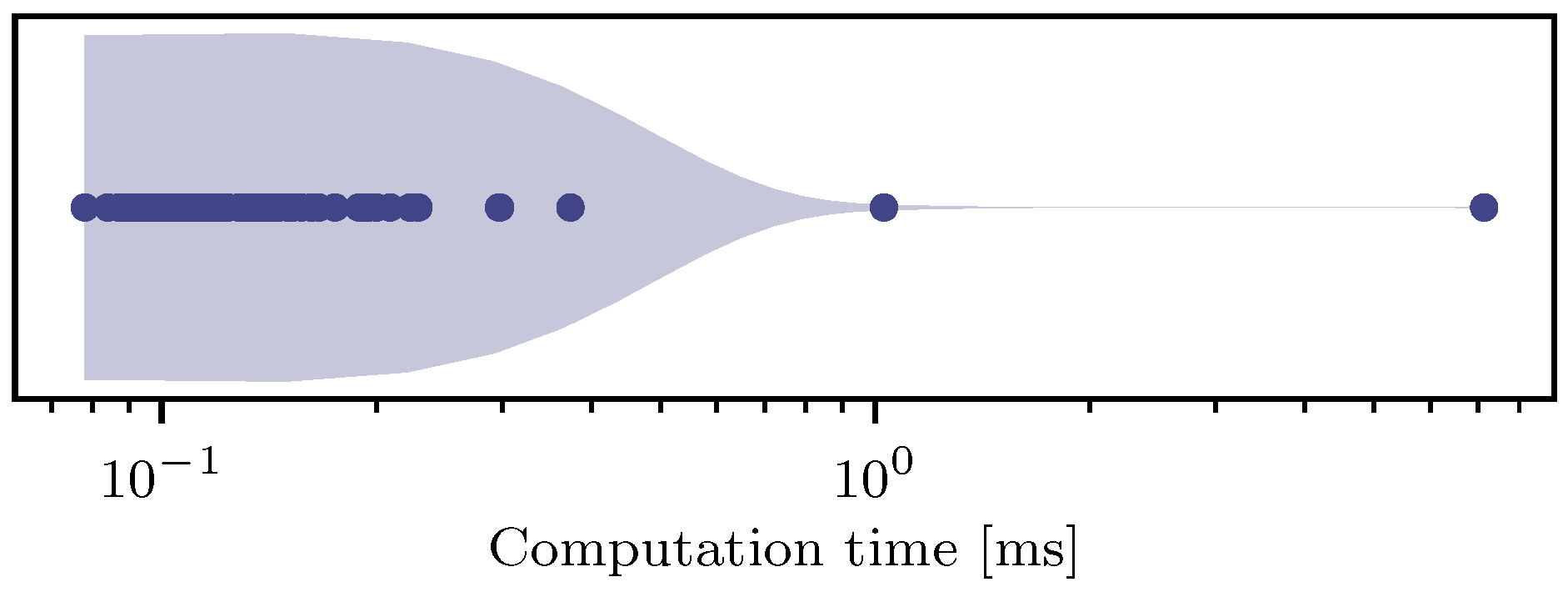
The efficiency of the algorithm is illustrated in Figure 9, showcasing remarkably low computational requirements. The average computation time is 0.2 . Even in instances where a considerably higher number of iterations is needed for feasibility correction, the computation times remain acceptable. It is essential to emphasize, however, that a conclusive evaluation of computation times can only be performed on a target vehicle.

Figure 9.
Computation times in milliseconds required at runtime to compute a trajectory for each lane center in the evaluation data set. The distribution as a violin plot and the individual samples are displayed.
5.2. Comparison to Re-Optimization
In Section 4.3, we present an approach utilizing the feasibility correction to compute trajectories at runtime, based on the results from precomputation. We compare this approach to the actual re-optimization of the re-parametrized optimal control problem. The precomputation phase for the re-optimization is the same. At runtime, the algorithm proceeds as follows. First, the best-fitting trajectory from the precomputation phase is selected, in the same manner as in Section 4.3. After that, the optimal control problem (21) parametrized with the lane center encountered at runtime is solved in the same way as during precomputation. The selected trajectory from precomputation is used as a good initial guess.
Both algorithms are evaluated on the evaluation data set. For each lane center in the evaluation data set, one trajectory is computed. The point in Frenet coordinates is always selected as an endpoint for the trajectories. This results in an optimal control problem (21) parametrized with the runtime lane center. The solution for this problem is approximated with the proposed sensitivity-based algorithm (Algorithm 2) and numerically solved by using the described re-optimization. The requirements regarding feasibility are the same for both approaches.
For one lane center, the trajectories obtained by applying the two algorithms are very similar. Table 1 depicts the differences between the related trajectories. All quantities usually exhibit a low difference. For instance, the position typically differs within the range of centimeters, which is likely much smaller than the utilized vehicle-dynamics model.

Table 1.
Comparison of the re-optimized and sensitivity-corrected trajectories. For each curve in the evaluation data set, trajectories were computed by using the two methods. Then, the maximum absolute difference per trajectory pair was determined. Finally, the mean and variance of these maxima were computed. The value range represents the minimum and maximum values present in any of the computed trajectories.
The average relative difference in the objective value between two related trajectories is , with a maximum relative difference of . This is an almost negligible difference. Still, it is noteworthy that the re-optimization process consistently results in a better objective value. This is due to the fact that the re-optimization approach typically computes a trajectory with a slightly smaller end time, which is the predominant term in the weighting of the objective function. The lower objective value in the re-optimization is reasonable, as this process involves significant computational effort to achieve actual optimality.
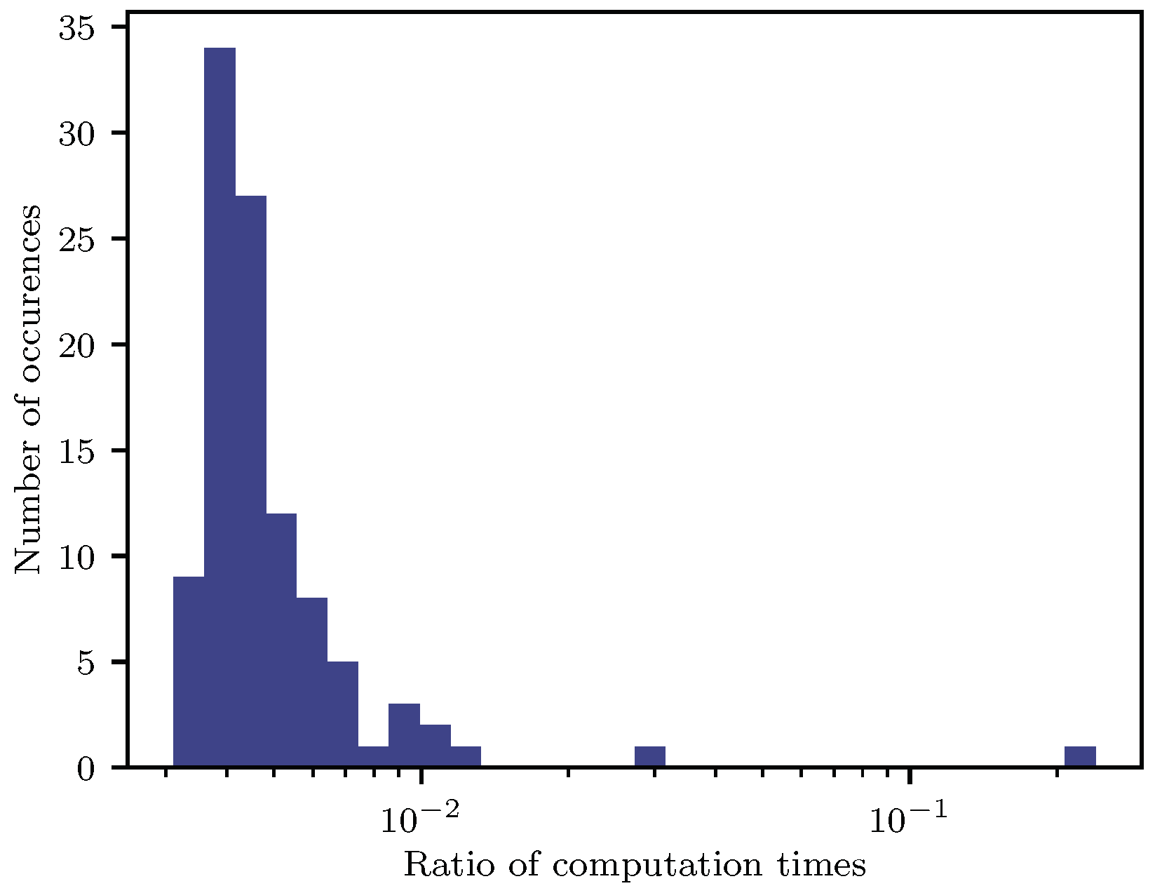
Figure 10 illustrates the effectiveness of the sensitivity approach. The sensitivity-based approach is much faster in all cases. For most of the computed trajectories, the sensitivity-based approach needs less than 1% of the computation time necessary for re-optimization. Even when feasibility correction needs over 700 iterations to converge, the approach is still about four times faster than re-optimization. Hence, the sensitivity-based update and correction algorithm outperform the re-optimization. While providing a similar solution quality, the computation time needed at runtime is much smaller. This comes at the cost of requiring more disk space to store the sensitivity matrices. However, on a real-time system, CPU efficiency is usually much more important than disk space, which is relatively inexpensive.

Figure 10.
Frequency of the ratios of related computation times between the sensitivity-based approach and the re-optimization. For each curve in the evaluation data set, one trajectory was computed using the sensitivity-based approach and one using re-optimization. The thereby observed computation time of the sensitivity-based approach was divided by the time needed for re-optimization.
The computation times of the sensitivity-based approach are within the interval . For re-optimization, the computation times are within . Hence, the relative range of computation times is much larger in the sensitivity-based approach. It seems to be more susceptible if the solution differs too much from the initial guess. There is also a theoretical basis for this observation. The sensitivity theorem (Theorem 3) guarantees the existence of a similar solution in a neighborhood of the reference. Hence, the difference in the parametrization should not be too large to assure low computation times and termination with a feasible solution.
The computation times needed for the re-optimization are similar to those observed during precomputation. For all mentioned computation times, it holds that the trajectory selection and loading of the precomputed resources require almost negligible computational effort compared to the feasibility correction and optimization process, respectively.
6. Conclusions
This paper contributes to the relatively sparse but highly relevant research on safe stop trajectory planning. The presented algorithm efficiently computes a feasible trajectory with minimal computational cost in real time for various road shapes. A crucial component in achieving this is the clustering method, which provides representative lane centers. This, in turn, allows for a precomputation phase, significantly reducing the algorithm’s execution effort when applied to an autonomous vehicle. However, this comes at the cost of additional memory requirements, as sensitivity matrices and the nominal solution itself have to be stored. The resultant trajectory ensures a rapid and comfortable halt in a safe position. The method achieves efficiency through feasibility correction and inherits the extensibility of optimal control in terms of problem formulation. This shows potential for improving the safety and comfort of autonomous vehicles. By means of this multistaged approach, some common drawbacks of nonlinear optimization can be mitigated. The precomputation does not underlie real-time requirements. Moreover, it is possible to spend additional effort during the offline phase for validation or to find globally optimal trajectories. Also, during runtime, a restriction to simple functions or convex problems is not necessary. As a novelty, the application of the feasibility correction method is evaluated on such a problem with a higher-dimensional parametrization of an optimal control problem. We showcase the efficiency of the algorithm in comparison to engaging in an entire NLP-solving process. While the solutions are almost identical, the computational effort needed at runtime is fundamentally smaller. The algorithm’s potential applications extend beyond trajectory planning, making it an interesting option for various use cases.
In preparation for actual application on a vehicle, it is recommended to define a grid of initial states and final positions. Trajectories are then computed for all combinations and cluster centers, ensuring a high degree of flexibility. The introduction of additional sensitivity parameters allows for the mitigation of errors arising from mapping an arbitrary initial state to a precomputed one.
It is important to note that the presented algorithm is tailored to scenarios where issues are detected early, and the current vehicle state aligns with traffic rules. Complex traffic scenarios, such as those involving intricate maneuvers like lane changes in consideration of other traffic participants, are not within its current scope. To enhance its capabilities in handling such complex situations, options include planning a substitute lane center around obstacles using polygons interpolating grid points, akin to the approach presented in [17]. Alternatively, a Voronoi diagram [42] or a simple graph-based algorithm could be employed to derive a well-suited lane center. Additionally, enhancing the robustness of the feasibility correction could be explored, for instance, by incorporating a line search method as proposed in [43].
Author Contributions
This article presents the results of J.L.’s master’s thesis, supervised by K.W.C. and C.M. C.B. was responsible for the project in which the thesis was created. All authors have read and agreed to the published version of the manuscript.
Funding
This research was supported by the German Aerospace Center (DLR) with financial means of the German Federal Ministry for Economic Affairs and Climate Action, project “MUTIG-VORAN” (FKZ: 50NA2202B).
Data Availability Statement
The data presented in this study are openly available in Mendeley Data at https://doi.org/10.17632/6vw8h8yf2t.1 (accessed on 22 December 2023).
Conflicts of Interest
The authors declare no conflicts of interest.
References
- Kriebitz, A.; Max, R.; Lütge, C. The German Act on Autonomous Driving: Why Ethics Still Matters. Philos. Technol. 2022, 35, 29. [Google Scholar] [CrossRef] [PubMed]
- Yurtsever, E.; Lambert, J.; Carballo, A.; Takeda, K. A Survey of Autonomous Driving: Common Practices and Emerging Technologies. IEEE Access 2020, 8, 58443–58469. [Google Scholar] [CrossRef]
- Badue, C.; Guidolini, R.; Carneiro, R.V.; Azevedo, P.; Cardoso, V.B.; Forechi, A.; Jesus, L.; Berriel, R.; Paixão, T.M.; Mutz, F.; et al. Self-driving cars: A survey. Expert Syst. Appl. 2021, 165, 113816. [Google Scholar] [CrossRef]
- González, D.; Pérez, J.; Milanés, V.; Nashashibi, F. A Review of Motion Planning Techniques for Automated Vehicles. IEEE Trans. Intell. Transp. Syst. 2016, 17, 1135–1145. [Google Scholar] [CrossRef]
- Paden, B.; Čáp, M.; Yong, S.Z.; Yershov, D.; Frazzoli, E. A Survey of Motion Planning and Control Techniques for Self-Driving Urban Vehicles. IEEE Trans. Intell. Veh. 2016, 1, 33–55. [Google Scholar] [CrossRef]
- Sharma, O.; Sahoo, N.; Puhan, N. Recent advances in motion and behavior planning techniques for software architecture of autonomous vehicles: A state-of-the-art survey. Eng. Appl. Artif. Intell. 2021, 101, 104211. [Google Scholar] [CrossRef]
- Boggio, M.; Novara, C.; Taragna, M. Trajectory planning and control for autonomous vehicles: A “fast” data-aided NMPC approach. Eur. J. Control 2023, 74, 100857. [Google Scholar] [CrossRef]
- Dempster, R.; Al-Sharman, M.; Rayside, D.; Melek, W. Real-Time Unified Trajectory Planning and Optimal Control for Urban Autonomous Driving Under Static and Dynamic Obstacle Constraints. In Proceedings of the 2023 IEEE International Conference on Robotics and Automation (ICRA), London, UK, 29 May–2 June 2023; pp. 10139–10145. [Google Scholar] [CrossRef]
- Li, G.; Zhang, X.; Guo, H.; Lenzo, B.; Guo, N. Real-Time Optimal Trajectory Planning for Autonomous Driving with Collision Avoidance Using Convex Optimization. Automot. Innov. 2023, 6, 481–491. [Google Scholar] [CrossRef]
- Meng, Y.; Wu, Y.; Gu, Q.; Liu, L. A Decoupled Trajectory Planning Framework Based on the Integration of Lattice Searching and Convex Optimization. IEEE Access 2019, 7, 130530–130551. [Google Scholar] [CrossRef]
- Zhang, X.; Liniger, A.; Borrelli, F. Optimization-Based Collision Avoidance. IEEE Trans. Control Syst. Technol. 2021, 29, 972–983. [Google Scholar] [CrossRef]
- Marcucci, T.; Petersen, M.; von Wrangel, D.; Tedrake, R. Motion planning around obstacles with convex optimization. Sci. Robot. 2023, 8, eadf7843. [Google Scholar] [CrossRef] [PubMed]
- Lin, Y.; Maierhofer, S.; Althoff, M. Sampling-Based Trajectory Repairing for Autonomous Vehicles. In Proceedings of the 2021 IEEE International Intelligent Transportation Systems Conference (ITSC), Indianapolis, IN, USA, 19–22 September 2021; pp. 572–579. [Google Scholar] [CrossRef]
- Meyer, H.F. Echtzeitoptimierung für Ausweichtrajektorien mittels der Sensitivitätsanalyse eines parametergestörten nichtlinearen Optimierungsproblems. Ph.D. Thesis, Universität Bremen, Bremen, Germany, 2016. [Google Scholar]
- Wang, H.; Huang, Y.; Khajepour, A.; Zhang, Y.; Rasekhipour, Y.; Cao, D. Crash Mitigation in Motion Planning for Autonomous Vehicles. IEEE Trans. Intell. Transp. Syst. 2019, 20, 3313–3323. [Google Scholar] [CrossRef]
- Salvado, J.; Custódio, L.; Hess, D. Contingency planning for automated vehicles. In Proceedings of the 2016 IEEE/RSJ International Conference on Intelligent Robots and Systems (IROS), Daejeon, Republic of Korea, 9–14 October 2016; pp. 2853–2858. [Google Scholar] [CrossRef]
- Wang, L.; Wu, Z.; Li, J.; Stiller, C. Real-Time Safe Stop Trajectory Planning via Multidimensional Hybrid A*-Algorithm. In Proceedings of the 2020 IEEE 23rd International Conference on Intelligent Transportation Systems (ITSC), Rhodes, Greece, 20–23 September 2020; pp. 1–7. [Google Scholar] [CrossRef]
- Svensson, L.; Masson, L.; Mohan, N.; Ward, E.; Brenden, A.P.; Feng, L.; Törngren, M. Safe Stop Trajectory Planning for Highly Automated Vehicles: An Optimal Control Problem Formulation. In Proceedings of the 2018 IEEE Intelligent Vehicles Symposium (IV), Changshu, China, 26–30 June 2018; pp. 517–522. [Google Scholar] [CrossRef]
- Büskens, C. Echtzeitoptimierung und Echtzeitoptimalsteuerung parametergestörter Probleme. Habilitation’s Thesis, Universität Bayreuth, Bayreuth, Germany, 2002. [Google Scholar]
- Knauer, M.; Büskens, C. Real-Time Optimal Control Using TransWORHP and WORHP Zen. In Modeling and Optimization in Space Engineering: State of the Art and New Challenges; Fasano, G., Pintér, J.D., Eds.; Springer International Publishing: Cham, Switzerland, 2019; pp. 211–232. [Google Scholar] [CrossRef]
- Nocedal, J.; Wright, S.J. Theory of Constrained Optimization. In Numerical Optimization; Springer: New York, NY, USA, 2006; pp. 304–354. [Google Scholar] [CrossRef]
- Fletcher, R. Practical Methods of Optimization, 2nd ed.; John Wiley & Sons: Chichester, UK, 2000. [Google Scholar] [CrossRef]
- Grippo, L.; Sciandrone, M. Introduction to Methods for Nonlinear Optimization; Springer International Publishing: Cham, Switzerland, 2023. [Google Scholar] [CrossRef]
- Pata, V. Fixed Point Theorems and Applications; Springer: Cham, Switzerland, 2019; pp. 75–80. [Google Scholar] [CrossRef]
- Fiacco, A.V. Sensitivity analysis for nonlinear programming using penalty methods. Math. Program. 1976, 10, 287–311. [Google Scholar] [CrossRef]
- Spellucci, P. Numerische Verfahren der Nichtlinearen Optimierung; Birkhäuser: Basel, Switzerland, 1993; p. 79. [Google Scholar] [CrossRef]
- Bringmann, K.; Künnemann, M.; Nusser, A. Walking the Dog Fast in Practice: Algorithm Engineering of the Fréchet Distance. J. Comput. Geom. 2021, 12, 70–108. [Google Scholar] [CrossRef]
- Alt, H.; Godau, M. Computing the Fréchet Distance between Two Polygonal Curves. Int. J. Comput. Geom. Appl. 1995, 5, 75–91. [Google Scholar] [CrossRef]
- Buchin, K.; Driemel, A.; van de L’Isle, N.; Nusser, A. klcluster: Center-Based Clustering of Trajectories. In Proceedings of the 27th ACM SIGSPATIAL International Conference on Advances in Geographic Information Systems, Chicago, IL, USA, 5–8 November 2019; pp. 496–499. [Google Scholar] [CrossRef]
- Ahmed, M.; Seraj, R.; Islam, S.M.S. The k-means Algorithm: A Comprehensive Survey and Performance Evaluation. Electronics 2020, 9, 1295. [Google Scholar] [CrossRef]
- Clemens, J.; Wellhausen, C.; Koller, T.L.; Frese, U.; Schill, K. Kalman Filter with Moving Reference for Jump-Free, Multi-Sensor Odometry with Application in Autonomous Driving. In Proceedings of the 2020 IEEE 23rd International Conference on Information Fusion (FUSION), Rustenburg, South Africa, 6–9 July 2020. [Google Scholar] [CrossRef]
- Langhorst, J. Rearranged and Subdivided Track Recording of a car within a Suburban Environment; Mendeley Data; V1. 2023. Available online: https://doi.org/10.17632/6vw8h8yf2t.1 (accessed on 22 December 2023).
- Höffmann, M.; Patel, S.; Büskens, C. Weight-Optimized NURBS Curves: Headland Paths for Nonholonomic Field Robots. In Proceedings of the 2022 IEEE 8th International Conference on Automation, Robotics and Applications (ICARA), Prague, Czech Republic, 18–20 February 2022; pp. 81–85. [Google Scholar] [CrossRef]
- Werling, M.; Ziegler, J.; Kammel, S.; Thrun, S. Optimal trajectory generation for dynamic street scenarios in a Frenét Frame. In Proceedings of the 2010 IEEE International Conference on Robotics and Automation (ICRA), Anchorage, AK, USA, 3–7 May 2010; pp. 987–993. [Google Scholar] [CrossRef]
- Polack, P.; Altché, F.; d’Andréa Novel, B.; de La Fortelle, A. The kinematic bicycle model: A consistent model for planning feasible trajectories for autonomous vehicles? In Proceedings of the 2017 IEEE Intelligent Vehicles Symposium (IV), Redondo Beach, CA, USA, 11–14 June 2017; pp. 812–818. [Google Scholar] [CrossRef]
- Folkers, A.; Wellhausen, C.; Rick, M.; Li, X.; Evers, L.; Schwarting, V.; Clemens, J.; Dittmann, P.; Shubbak, M.; Bustert, T.; et al. The OPA3L System and Testconcept for Urban Autonomous Driving. In Proceedings of the 25th IEEE International Conference on Intelligent Transportation Systems (ITSC), Macau, China, 8–12 October 2022; pp. 1949–1956. [Google Scholar] [CrossRef]
- Betts, J.T. Practical Methods for Optimal Control and Estimation Using Nonlinear Programming, 2nd ed.; Society for Industrial and Applied Mathematics: Philadelphia, PA, USA, 2010; pp. 129–134. [Google Scholar]
- Dubins, L.E. On Curves of Minimal Length with a Constraint on Average Curvature, and with Prescribed Initial and Terminal Positions and Tangents. Am. J. Math. 1957, 79, 497–516. [Google Scholar] [CrossRef]
- Walker, A. Dubins-Curves: An Open Implementation of Shortest Paths for the Forward Only Car. Version from 14 March 2018. Available online: https://github.com/AndrewWalker/Dubins-Curves (accessed on 27 April 2023).
- Breuer, S.; Rohrbach-Kerl, A. Fahrzeugdynamik: Mechanik des bewegten Fahrzeugs; Springer Vieweg: Wiesbaden, Germany, 2015; p. 145. [Google Scholar] [CrossRef]
- Büskens, C.; Wassel, D. The ESA NLP Solver WORHP. In Modeling and Optimization in Space Engineering; Fasano, G., Pintér, J.D., Eds.; Springer: New York, NY, USA, 2013; pp. 85–110. [Google Scholar] [CrossRef]
- Bhattacharya, P.; Gavrilova, M.L. Voronoi diagram in optimal path planning. In Proceedings of the 4th International Symposium on Voronoi Diagrams in Science and Engineering (ISVD), Pontypridd, UK, 9–11 July 2007; pp. 38–47. [Google Scholar] [CrossRef]
- Ferry, M.W.; Gill, P.E.; Wong, E.; Zhang, M. A class of projected-search methods for bound-constrained optimization. Optim. Methods Softw. 2023. [Google Scholar] [CrossRef]
Disclaimer/Publisher’s Note: The statements, opinions and data contained in all publications are solely those of the individual author(s) and contributor(s) and not of MDPI and/or the editor(s). MDPI and/or the editor(s) disclaim responsibility for any injury to people or property resulting from any ideas, methods, instructions or products referred to in the content. |
© 2024 by the authors. Licensee MDPI, Basel, Switzerland. This article is an open access article distributed under the terms and conditions of the Creative Commons Attribution (CC BY) license (https://creativecommons.org/licenses/by/4.0/).