Article

Planning Speed Mode of All-Wheel Drive Autonomous Vehicles Considering Complete Constraint Set

Department of Civil Engineering, Toronto Metropolitan University, 350 Victoria Street, Toronto, ON M5B2K3, Canada
*
Author to whom correspondence should be addressed.
Vehicles 2024, 6(1), 191-230; https://doi.org/10.3390/vehicles6010008
Submission received: 26 October 2023 / Revised: 8 January 2024 / Accepted: 9 January 2024 / Published: 12 January 2024
(This article belongs to the Topic Vehicle Dynamics and Control)

Abstract

:
The study aims to improve the technique of motion planning for all-wheel drive (AWD) autonomous vehicles (AVs) by including torque vectoring (TV) models and extended physical constraints. Four schemes for realizing the TV drive were considered: with braking internal wheels, using a rear-axle sport differential (SD), with braking front internal wheel and rear-axle SD, and with SDs on both axles. The mathematical model combines 2.5D vehicle dynamics model and a simplified drivetrain model with the self-locking central differential. The inverse approach implies optimizing the distribution of kinematic parameters by imposing a set of constraints. The optimization procedure uses the sequential quadratic programming (SQP) technique for the nonlinear constrained minimization. The Gaussian N-point quadrature scheme provides numerical integration. The distribution of control parameters (torque, braking moments, SDs’ friction moment) is performed by evaluating linear and nonlinear algebraic equations inside of optimization. The technique proposed demonstrates an essential difference between forecasts built with a pure kinematic model and those considering the vehicle’s drive/control features. Therefore, this approach contributes to the predictive accuracy and widening model properties by increasing the number of references, including for actuators and mechanisms.

1. Introduction

Usually, planning and tracking stages are separated as hierarchical components; however, a complex approach is also possible [1]. The planning quality reduces the time cost needed for optimizing the control at the tracking stage, as well as minimizes the probability of AV’s unstable motion modes. The variant of decomposing path and speed planning is caused by the need to decrease the number of space-time variations during optimization when the number of constraints increases. Thus, in studies such as [2], first, a visible foresighted trajectory was generated, and the speed plan was then optimized with respect to space. Afterward, the optimal control problem was formulated in the space instead of the time domain.
Models. The problem of smoothed speed arose as a need for high-quality control preventing the appearance of sudden loads and unstable transients. Some studies as [3] attempted to compose speed plans based on cubic polynomials in such a way as to ensure the continuity of accelerations at the transition nodes under conditions of minimizing the jerk. However, the function inflections did not occur directly in the nodes, which led to some excesses of the preset limits followed by the need for complicating the model to compensate for this fluctuation effect. This approach allows obtaining continuous speed values at any point, considering the initial and final values.
The range of models used to represent the AV at the planning stage is quite wide and depends on the control objective. Kinematic models are the simplest and meet the requirements of maximum performance. The bicycle model [4] is traditional and has proven itself well when using model predictive control (MPC). The best quality corresponds to the state-space kinematic models with the control actions such as jerk and the steered wheels’ angles [5].
Dynamic models can be both complex and simple to control a single aspect. For example, in [6] a longitudinal dynamic model is identified to tune a low-level speed-tracking controller. In [7] a simplified constrained model uses a second-order integrator to match the feasible AV dynamic behavior. This also includes speed planning to automatically adjust the vehicle’s capabilities relative to the road conditions. The yaw, roll, and pitch of AV body’s DOFs, each wheel’s dynamics based on slip ratios, and Pacejka’s combined slip tire model are computed. The comparison of kinematic and dynamic models concerning experimental data [4] shows different statistics of forecast errors, including the effect of discretization error accumulation. In [8], a search-based method solves the problem with nonlinear and unstable dynamics.
Objective functions determine the planning and control strategies. Most studies proceed from the control strategy regarding minimizing the motion time while keeping the vehicle within roadway boundaries [9]. Thus, in [10], the time-optimal trajectory around a racetrack is obtained by solving a minimum lap time problem (MLTP) for a racing vehicle. In [11], the path planning strategy includes preventing rear-end collisions during overtaking while minimizing traveling time.
Controllers. Different types of controllers are used for both planning and tracking. The class of controllers based on MPC can be considered the most used that allows obtaining high-quality forecasts due to a combination of hard and soft constraints [5]. Another popular class is the LQR-type controllers. For increasing performance and overcoming physical limitations, a technique can be represented by the augmented Lagrangian framework [6], which refers to iterative LQR (ILQR) and Constrained Iterative LQR (CILQR), respectively. In [12], the sliding mode control (SMC) calculates the total driving force for longitudinal control. In [7], the reference path is followed by low-level tracking using PID controllers. In [13], a learning-based Interaction Point Model (IPM) describes the interaction between agents. In [9], the Nonlinear Model Predictive Control (NMPC) strategy was aimed at controlling a small-scale car model for autonomous racing competitions. Study [6] presented a hierarchical framework with neural physics-driven models to enable the online planning and tracking of minimum-time maneuvers. A lateral speed prediction model for high-level motion planning was considered with economic nonlinear model predictive control (E-NMPC). In [1], a linear parameter-varying (LPV) MPC was deployed for AV trajectory tracking and compared with the linear MPC. The outcomes satisfy the processing rate and high-precision criteria, including safely avoiding obstacles. In [14], the path-following control strategy was based on the linear quadratic regulator (LQR) to compare the performance of models. In [12], the MPC controller was used to calculate the steering wheel angle and the total yaw moment for lateral control, and the sliding mode control (SMC) was used to calculate the total driving force for longitudinal control.
ADAS. Note that the problem of speed planning is typical not only for AVs but also for ADAS systems. In [5], it was proposed to form a speed profile for functioning the adaptive cruise control (ACC) based on MPC. The study [15] considered a preview servo-loop speed control algorithm to achieve smooth, accurate, and computationally inexpensive speed tracking for connected automated vehicles (CAVs). A classic PID with an optimal controller was implemented in an automated vehicle platform for lowering speed-tracking errors, mitigating operations, and smoothing brake/throttle activations. The paper [11] proposed a system for speed planning using MPC to estimate the vehicle overtake safety while controlling the maneuver for a dynamic vehicle model.
Paper [16] presented an AV’s trajectory planning and speed control algorithm for static traffic agent avoidance in multi-vehicle urban environments. Decision-making and motion planning frameworks were presented considering both the preceding static and surrounding vehicles. Paper [17] considers hierarchical architecture for decision making, motion planning, and control for an autonomous racing vehicle. The supervisor determined whether the subject vehicle should stay behind the preceding vehicle or start overtaking. A high-level trajectory planner generated the desired path and velocity profile in a receding horizon mode. A low-fidelity kinematic vehicle model was utilized for planning, and a low-level trajectory tracker based on MPC and dynamic vehicle model generated the lateral and longitudinal control inputs.
Some studies implemented the use of four-wheel models with increased degrees of freedom, refined tire models, actuators, etc. Thus, in [14], the question of tire dynamics’ influence on vehicle dynamics’ control was raised. The influence of tire nonlinearity on path offset was revealed. In [12], the longitudinal and lateral motion control for the four-wheel independent drive intelligent vehicle was designed: the upper layer was the motion controller, and the lower layer was the control distributor. In [8], complex dynamics in a predictive manner were applied to achieve optimal robot behavior in dynamic scenarios. In paper [18], a new real-time motion planning technique for an autonomous mobile robot is proposed considering actuator capacities’ limits and tire-ground adhesion constraints.
Actuators. Study [9] includes a simple drivetrain model in the optimization problem to limit the lateral and longitudinal forces acting on a car. An Autonomous Emergency Braking Pedestrian (AEB-P) was introduced in [19] to prevent collisions between vehicles and pedestrians. The emergency brake planner generates vehicle deceleration followed by tracking the trajectory, where the PI-controller was adapted to provide the optimum braking force. In [15], the brake/throttle control laws were introduced in five parts: three feedback controls of system states and two feedforward items previewing road slope and target speed. Study [20] proposes a clothoid-curve-based trajectory tracking control method to solve the problem of tracking errors caused by the discontinuous curvature of the control curve calculated by simple algorithms. The parameters of clothoid reference curves are tied to the vehicle’s safe motion constraints.
Despite the intensive studies on motion planning, in our opinion, there still are some issues that can be conditionally divided into three parts: vehicle model, restrictions, and planning techniques.
Vehicle model. Note that most studies in the field of AV motion planning are focused on generating reference curves using relatively simple (often kinematic bicycle) models. However, the motion planner’s high performance does not yet mean high forecast quality. The most important indicators are the prognosis feasibility and ensuring good accuracy in reflecting features of a specific vehicle design. Considering the intensive use of control systems in modern vehicles (for example, traction distribution), it is often not enough to obtain the trajectory and kinematic parameters’ references. Moreover, the desirable parameters themselves may significantly depend on the technologies used in a real vehicle. For example, the distribution of drive torques between the same axle’s wheels can be carried out through a symmetrical differential, through a sport differential (torque vectoring), and by activating the inner wheels’ brakes. All three options will cause different axle drive power, different traction and lateral forces, the tire–road adhesion degree, and, as a result, affect differently on forming the yaw moment. In a classic uncontrolled AWD drivetrain, a wheel with the worst adhesion conditions limits the traction potential. And vice versa, in transmissions design with individual wheel control, the maximum realization of total adhesion potential is possible. In the case of using a standard vehicle model, there will be no difference between these two variants when speed is the planning object. If an extended model is used, including the drive type and redistribution of vertical reactions, then, as shown in our previous articles, the difference between predictions of kinematic parameters may be significant especially for cases with low tire adhesion. Thus, this study’s target consists of composing an inverse vehicle dynamic model that allows estimating physical factors based on the kinematic parameters.
A set of constraints is a critical factor in reflecting the realism of forecasting and the optimization procedure’s performance. On the one hand, increasing the number of restrictions complicates the mathematical optimization model; on the other hand, narrowing the boundaries of AV motion parameters contributes to diminishing solution iterations and time costs.
When using a conventional kinematic model, constraints are also basically kinematic (linear and angular velocities, linear and angular accelerations, jerk, etc.), which does not always correspond to natural physical limits. For example, many researchers use a constant upper acceleration limit without relating it to the throttle response properties (speed–acceleration) for a specific vehicle design. At the same time, the traction potential decreases with speeding even for the case of electric drive, which especially should be considered for a medium-speed range.
The physical limitations are the most important but require an extended vehicle model. First, these restrictions are responsible for preventing motion instability, critical modes of vehicle-road interaction, and are associated with the design solutions for distributing the power by wheels. Controlling the tires’ adhesion limits is the most important aspect, requiring predicting both a redistribution of normal reactions and torques on wheels. In turn, the torque depends on the drive design and control. In addition, pure kinematic models do not allow direct operation with longitudinal and lateral slip. Nevertheless, it is possible to indirectly estimate tires’ slip angles and lateral deformations followed by including them in the constraints.
Safety restrictions. Most often, this includes speed limits when approaching moving and static obstacles. Within this planning technique, we suppose that a trajectory considering obstacles and speed mode has already been built. Therefore, in the framework of this study, we assume that the AV uses a safe space for realizing a maneuver. As a safety measure, the body roll angle caused by lateral inertia forces is applied. Restricting the maximum roll angle, limitations on lateral acceleration are automatically imposed.
Thus, in advance, we proceed from the fact that growth in the number of restrictions positively affects the rapidity and quality of forecasting the AV motion.
Planning technique. Here, the most important requirements concern ensuring the smoothness and unambiguousness of predicted functions. The most common approach implies using polynomials that describe the change in speed concerning time along a trajectory section. However, this does not always lead to a qualitative consistency between the speed and curvature derivatives involved in the formation of kinematic parameters such as jerk and angular acceleration. That is, there may be disruptions in the piecewise representation of these functions. This, in turn, does not contribute to the possibility of using inverse dynamics to determine the force factors acting on the vehicle. In this regard, our method consists of using an inverse approach, when instead of speed its second derivative is directly modeled by smooth functions. In this case, the continuity and smoothness of the vehicle’s linear and angular accelerations will be guaranteed.
Figure 1 shows a general approach scheme reflecting the modeling stages and the parameters used. The SQP optimization ensures iterative process, within which kinematic, dynamic, and physical parameters are evaluated to form optimization criteria and constraints. To model vehicle kinematics, the inverse method is used, allowing the representation of the longitudinal speed function via finite elements. The external data are the preset boundary values of the kinematic parameters, initial conditions, and the precalculated trajectory model. The SQP-loop at each iteration generates a vector of nodal parameters for the longitudinal speed’s second derivative. A simple and smooth form of the speed function is obtained by double numerical integration. After evaluating accelerations, the distribution of normal reactions over the wheels can be found. Using the AWD transmission model, vehicle steerability and nonlinear tire models, and algorithms for controlling traction distributing actuators, the inverse dynamics problem is solved, followed by determining the needed longitudinal and lateral forces and estimating degrees of longitudinal and total tire adhesion use. Knowing the lateral forces and accelerations allows estimating the equivalent sideslip angles, tire lateral deformations, and the body roll angle, including them in a set of nonlinear constraints. As a result, the optimization output contains kinematic, dynamic, and physical parameters, as well as the necessary control for actuators.

2. Existing 2.5D Vehicle Dynamics Model

2.1. Model Scheme

Let us present the schemes to reflect the active forces, geometric, and kinematic parameters needed for parametrizing the AV model (Figure 2).

2.2. Trajectory-Based Vehicle Kinematics

Assuming the maneuver trajectory is preoptimized, we outline the main points of the ideal vehicle kinematics providing better controllability and motion stability. At the same time, the main task consists of linking the kinematic parameters with the trajectory’s geometric ones, ensuring the continuity of their derivatives (Figure 2a).
Mass center speed V is directed by the trajectory tangent and may be expressed as follows
V = V ζ u ζ + V μ u μ = V x u x + V y u y
where u ζ , u μ , Vζ, Vμ = unit vectors and speed components of the vehicle local coordinate system ζμ; u x , u y , Vx, Vy = unit vectors and speed components of the fixed (global) coordinate system xy.
The absolute speed V may be decomposed with projections Vx and Vζ tied through the tangent angle α and central slip angle β. Then,
V = d s d t = d s d x d x d t = V x c o s α = V ζ cos β , V x = V ζ cos α cos β
The first and second derivatives of Vζ may be found as follows
d V ζ d t = d V ζ d x d x d t = d V ζ d x V x , d 2 V ζ d t 2 = d 2 V ζ d x 2 V x 2 + d V ζ d x d V x d x V x
The derivative of Vx concerning the x-coordinate is
d V x d x = d V ζ d x + V ζ d β dx tan β d α dx tan α cos α cos β
Lateral Speed Vμ is geometrically tied with the longitudinal speed Vζ by the central slip angle β
V μ = V ζ tan β
Its time derivative
d V μ d t = d V μ d x d x d t = d V μ d x V x , d V μ d x = d V ζ d x tan β + V ζ d β dx sec 2 β
Yaw Rate is the yaw angle ϕ = αβ derivative in the current global coordinates. Thus,
ω = d ϕ d t = d ϕ d x d x d t = d ϕ d x V x , d ω d x = d d x d ϕ d x V x = d 2 ϕ d x 2 V x + d V x d x d ϕ d x
Angular acceleration ε is derived from the yaw rate ω concerning time
ε = d ω d t = d ω d x d x d t = d ω d x V x = d 2 ϕ d x 2 V x 2 + d V x d x ω
Accelerations in the local vehicle coordinate system ζμ are
a = d V d t = a ζ a μ T u ζ u μ , a ζ a μ = d V ζ / d t d V μ / d t + ω V μ V ζ
Jerks in the vehicle coordinate system are
j = d a d t = j ζ j μ T u ζ u μ = d 2 V ζ d t 2 2 d V μ d t + V ζ ω ω ε V μ d 2 V μ d t 2 + 2 d V ζ d t V μ ω ω + ε V ζ T u ζ u μ
Velocities and accelerations at the wheels’ centers are needed for assessing the forces acting in the tire–road contacts. Let us introduce designations
U = 0 1 1 0 , U U = 1 0 0 1 = E 2 , r j = r j ζ r j μ , v = V ζ V μ , v j = v ζ j v μ j , H · = cos · sin · sin · cos · , u ζ j u μ j = H θ j u ζ u μ , u ζ u μ = H T θ j u ζ j u μ j
where E2 = identity matrix of dimension 2 × 2, rj = vector of j-th wheel center’s coordinates in the AV local coordinate system, v j = vector of j-th wheel center’s velocities in the wheel local coordinate system, H = rotational matrix, θj = angle of j-th wheel turn, and u ζ j , u μ j = unit vectors of the j-th wheel local coordinate system.
Speed and Acceleration vectors in the center of j-th wheel’s local coordinates
v j = v ζ j v μ j = H θ j v + ω U T r j , a j = a ζ j a μ j = H θ j a + ε U T ω 2 E 2 r j
Rotation angles of steered wheels can be determined as Ackerman’s angles subject to that the trajectory curvature K is much less than the maximum possible. Thus,
θ 1 = a r c c o t cos β K B 12 B 13 2 B 12 , θ 3 = a r c c o t cos β K B 12 + B 13 2 B 12

2.3. Vehicle Dynamics

2.3.1. Body Pseudo-Roll

To enhance the influence of transversal forces on vehicle safety and redistributing vertical reactions, the body roll phenomenon may also be used. It can be estimated using the simplest scheme, as depicted in Figure 2b. Assuming that the vehicle body mass center can deviate on the angle ψ relative to a roll center, the dynamics equation for the balance of moments is derived as follows
M ψ = r ψ × P μ + m b g = r ψ × a μ + g m b
where mb = mass of the vehicle body, rψ = roll lever, g = gravity acceleration constant.
Performing a cross product, obtain
M ψ u ψ = r ψ u r × u μ a μ u z g m b = r ψ a μ cos ψ + g   B 12 B r sin ψ m b u ψ
where u ψ , u r = unitary vectors along the roll axis and roll lever, respectively,
B r = B 12 2 + h 24 h 13 2
At the same time, the moment modulus is proportional to the angle ψ and the angular stiffness coefficient kψ
M ψ = k ψ ψ
Equating the modules of Equations (15) and (16), we obtain for the angle ψ
ψ = m b r ψ k ψ a μ cos ψ + g   B 12 B r sin ψ
Supposing the angle ψ to be small, the expression of Equation (17) may be reduced to the linear form. If the constant part is denoted as pψ, then the roll angle will be a linear function of the lateral acceleration
ψ = p ψ a μ , p ψ = 1 / k ψ m b r ψ g B 12 B r
The roll lever rψ (Figure 2c) can be estimated based on dependencies [21]
r ψ = h g B 12 B r h 24 c + h 13 b / B r h g b h 13 + c h 24 / B 12
where h13, h24 = ordinates of the roll centers of the front and rear suspensions, respectively (double wishbone suspensions are usually slightly below the wheel-center axis).
The angular stiffness of suspensions can be defined as follows
k ψ = k s 13 + k s 24 , k s 13 = 1 2 B 13 2 k s f , k s 24 = 1 2 B 24 2 k s r
ksf, ksr = reduced stiffness of independent front and rear suspensions, respectively.
The suspension stiffness can be estimated from the lowest natural frequency of free oscillations. Then,
k s f , r = 4 π 2 m s f , r f s f , r 2
msf,r = sprung masses distributed on every single front and rear suspensions, respectively, fsf,r = natural oscillation frequencies of sprung masses (for modern cars fs = 0.6…1.3 Hz).

2.3.2. Redistribution of Vertical Reactions

The distribution of vertical reactions is the basic factor determining the wheel’s potential in transmitting longitudinal and transversal forces. The nature of the longitudinal and transverse accelerations generated during optimization should be such as to provide an approximate constancy of adhesive properties without violating the imposed restrictions. Considering (Figure 2a), the balance of moments in the vehicle’s longitudinal plane can be derived as follows
l x cos γ + h g e sin γ + a ζ g m g + e P a d h a + e e M μ R z a B 12 = 0 2
where γ = angle of road slope, and
R z a = R z f R z r , M μ = M μ f M μ r , l x = b c , e = 1 1 , B 12 = b + c
Provided that for most of the moving time γ ≈ 0, Equation (22) may be reduced to
l x + h g e a ζ g m g + e P a d h a + e e M μ R z a B 12 = 0 2
Wheel rolling resistance moments Mr can be partially estimated by omitting kinematic losses (no sliding) and seeing only power losses. However, this requires a normal load value on each wheel. To simplify, we may consider the moments from conditionally paired front and rear wheels. Then,
M r f r = R z f r r w f r f r f r
where rwf(r) = dynamic radius of front (rear) wheel, frf(r) = coefficient of front (rear) rolling resistance.
Using the steered wheels’ average turning angle θf(r), we obtain
M μ f r = M r f r cos θ f r
Then, the rolling resistance moments can be derived in terms of vertical reactions
M μ = R z f r w f f r f cos θ f R z r r w r f r r cos θ r = r w f f r f cos θ f 0 0   r w r f r r cos θ r R z f R z r = m μ R z a
Thus, Equation (23) may be rewritten in the form
R z a = B 12 E 2 e e m μ 1 l x + h g e a ζ g m g + e P a d h a
Assuming that the increments of normal reactions on the right and left sides are equal due to the vehicle symmetry relative to the longitudinal plane, we obtain the vector of dynamic reactions caused by the longitudinal acceleration
R z ζ = Δ R z ζ 1 Δ R z ζ 2 Δ R z ζ 3 Δ R z ζ 4 = 1 2 1 0 0 1 1 0 0 1 R z f R z r , R z ζ = 1 2 E 2 E 2 R z a
The distribution of vertical reactions along the sides, considering Figure 2d, may be derived from the equations of moments’ equilibrium relative to each wheel’s contact center. Designate
μ w = 1 2 B 13 B 24 B 13 B 24 ,   e = 1 1 1 1 ,   R z μ = Δ R z μ 1 Δ R z μ 2 Δ R z μ 3 Δ R z μ 4 ,   μ = e μ w T ,   Y = μ μ T ,   M ζ = e M ζ r + M ζ l
where Mζr, Mζl = overturning moment from the right and left vehicle sides.
Since the tire deformations in the lateral direction are omitted at this stage, only the rolling resistance of moment components is taken as the wheel overturning moment. Considering them along the axes, we obtain
M ζ f r = M r f r sin θ f r , M ζ = e M r f sin θ f + M r r sin θ r = e M r f sin θ f
Since the model assumes a pseudo-roll, which causes some displacement of the mass center (Figure 2b), the gravity effect can be clarified with the moment mb·g·rψ·sin(ψ) ≈ mb·g·rψ·ψ, where the pseudo-roll angle can be preliminarily estimated from the lateral acceleration. The matrix equation of the moment balance relative to the centers of the wheels’ contacts is represented as follows
Y R z μ + m a μ h g + M ζ + m b g r ψ ψ = 0
The matrix Y is singular because of the vehicle symmetry. Therefore, the pseudo inverse matrix Y+ is used for redistributing vertical reactions caused by the lateral acceleration. Then,
R z μ = Y + m a μ h g + m b g r ψ ψ + M ζ
Thus, the vector of vertical reactions is a combination of both distributions
R z = R z ζ + R z μ

2.3.3. Pseudo-Tires’ Slip Angles

Since a kinematic model is used for speed planning, which does not imply the tire’s side elasticity and sideslip, the motion trajectory may acquire a certain excessively ideal character. For partial leveling of this drawback, it is possible to estimate in the first approximation the values of tires’ lateral sideslips and deformations stipulated by the speed Vζ and acceleration aμ. Since the lateral accelerations and speeds at the wheels’ centers are known by Equation (12), it is possible to evaluate the lateral forces required for stable motion. To do this, briefly consider the main factors affecting the lateral sideslip.
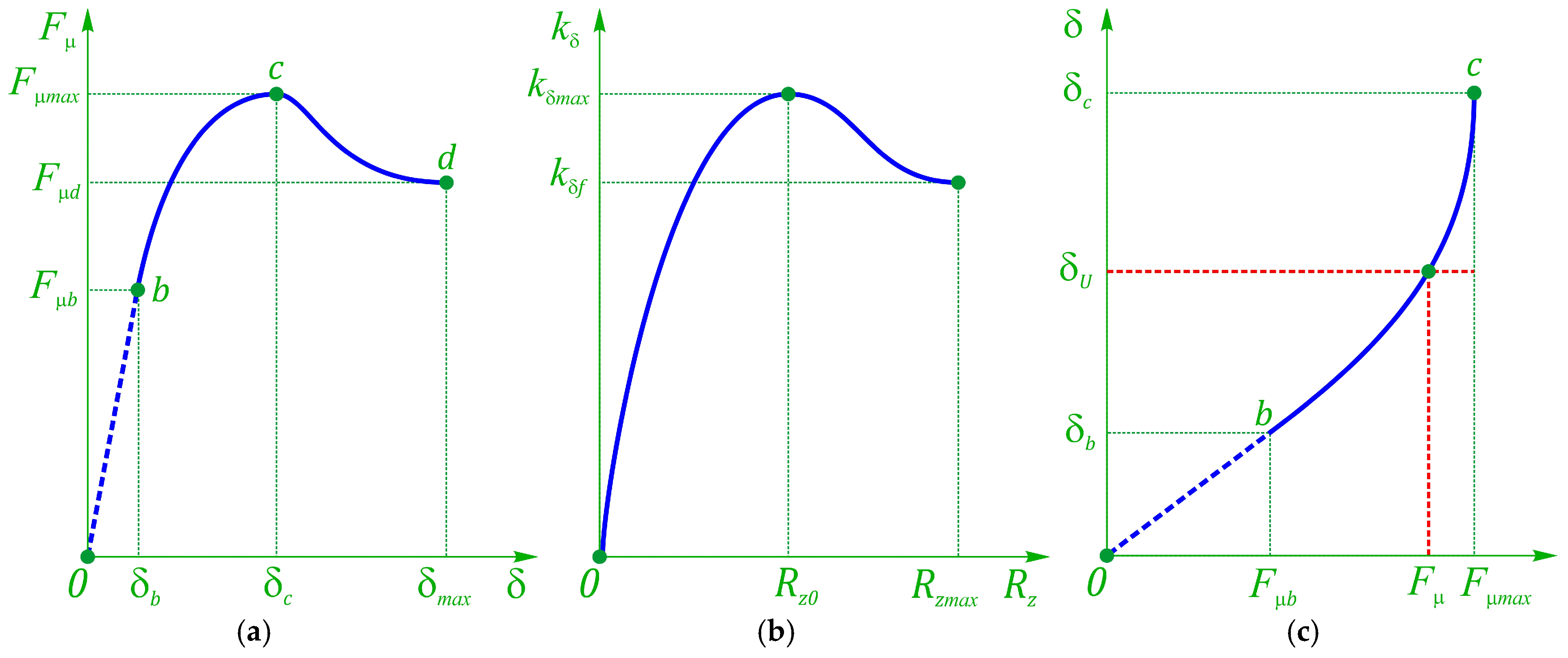
When the slip angel δ changes from zero to some value b (segment 0b, Figure 3a), which is different for various tires, normal loads, and tire–road friction coefficients, the dependence Fμ = f(δ) is almost linear,
F μ = k δ δ
This segment corresponds to Fμ, at which the slippage is small.
The segment bc corresponds to the Fμ values, at which the slip occurs on a significant part of the tire’s contact area, and the more intensively the larger δ is. At point c, the force Fμ reaches its maximum value according to the adhesion condition, and in segment cd, it is determined by the equality Fμmax = Rzφμmax, where φμmax is the coefficient of transverse adhesion. Conditionally, in segment 0c, the wheel lateral movement caused by the force Fμ is called the sideslip, and in segment cd it is called the pure slip. The angle value δc, at which sliding begins, depends on the tire structure, normal load, coefficient φμmax, and other factors. Usually, for a dry road surface δc = 12–20°. In terms of kinematics, it does not matter for what reason the velocity vector deviation from the rotation plane occurs; therefore, the angle δ is formed by the components of the wheel’s longitudinal and transverse speeds over the entire range 0d.
The vehicle steerability is largely defined by the dependence kδ = f(Rz) (Figure 3b). For passenger vehicles, kδ has a maximum value kδmax when the force Rzopt is close to that corresponding to the vehicle’s gross weight Rz0. The coefficient kδ value depends on the coefficient φμmax. In segment 0b, the coefficient kδ is practically independent of the coefficient φμmax. However, the smaller φμmax, the smaller the angle δ value corresponding to the point d. On a dry road surface with a force Rz corresponding to standards for a given tire, it can be taken equal to δb ≈ 3–4°. Formula (35) is also valid for the section bc, at which kδ = f(δ) or kδ = f(Fμ) (Figure 3c). In this segment, the smaller φμmax, the smaller the values of kδ.
During the vehicle motion, the change in value and direction of the wheel’s longitudinal force Rζ affects the dependence Fμ = f(δ). With an increase in Rζ/Rz, to obtain the same angles δ in the traction mode, a smaller force Fμ is needed. In the braking mode, at small Rζ/Rz, its increase leads to a slight growth in the force Fμ, and at larger Rζ/Rz—the Fμ decreases. If Rζ/Rz is small, then the effect of longitudinal forces Fμ = f(δ) is insignificant. The longitudinal forces exert the greatest influence at values of the Rζ forces that are close in value to the maximum adhesion.
Slippage starts when Rmax = Rzφmax. In this case, the adhesion coefficient φmax depends on the slip direction of the contact patch relative to the road surface, which coincides with the direction of the reaction R. When sliding in the rotation plane, the adhesion coefficient is φζ, and in the transverse direction φμ.
With the onset of lateral slip, slippage in the wheel’s rotation plane also occurs. The ratio between the speeds of the lateral and longitudinal slips is the same as between the lateral and longitudinal reactions.
Antonov D. A. [21] proposed considering the influence of various factors on the coefficient kδ by multiplying kδmax with several correction factors. With the wheel’s straight-line steady rolling on an even, nondeformable road surface
k δ = k δ m a x q φ q z q ζ q p
where kδmax = the driven wheel’s slip resistance coefficient on the dependence Fμ = f(δ) linear section at the maximum values of the dependences kδ = f(Rz) or kδ = f(pa). qφ = correction factor considering the slip resistance dependence on the angle δ while moving on roads with different φ (non-linear dependence Fμ = f(δ)), qz = correction factor considering the effect of normal load deviation from the optimum one, qζ = correction factor considering the influence of longitudinal forces on kδ, and qp = correction factor considering the effect of the tire’s air pressure pa deviation from the optimal pressure (supposedly neglected and equals 1).
The coefficients can be calculated from the following dependences
q φ = a r c t a n λ φ δ δ 0 λ φ δ δ 0 , λ φ = π k δ 0 2 φ μ R z
where kδ0 = the slip resistance factor at a given value of Rz in a linear section Fμ = f(δ), and δ0 = the slip angle corresponding to the transition from a linear section to a nonlinear section (regarding b). Usually, δ0 = 0.025–0.035 rad.
q z = 0.4 λ z 3 1.8 λ z 2 + 2.4 λ z , λ z = R z R z o p t R z R z 0
q ζ = 1 R ζ / R ζ m a x 2 1 + 0.375 φ ζ , φ ζ = R ζ R z , R ζ m a x = R z φ ζ m a x
The dependence Fμ = f(δ) corresponds to the steady-state wheel rolling when Fμ = const and the trajectory of the wheel’s center is a straight line. In most cases, this dependence can also be used to study controlled motion at Fμ = f(t).
As mentioned, the linear segment of the tire’s lateral force characteristic continues to the slip angle of about δb ≈ 3–4° under a static load and dry surface at the wheel’s driven mode, providing the maximum potential of φμ. Since a decrease in φμ leads to a reduction in kδ0, the angle δb also drops. Assuming a linear dependence, the initial angle δ0 of the linear zone can be calculated as
δ 0 0.4 R z φ μ k δ 0 δ b
Thus, the lateral force, considering the load, adhesion, and traction use, can be expressed as a dependence on the slip angle as
F μ = f δ = k δ 0 δ , 0 δ   δ 0 k δ 0 q φ δ , δ > δ 0   , k μ 0 = k δ m a x q z q ζ q p
This nonlinear characteristic will be used for determining the wheels’ side reactions.

2.3.4. Pseudo-Tires’ Lateral Deformations

The tire lateral deformation also directly affects the wheel slip angle and the trajectory offset relative to the rigid wheel option. At the same time, to ensure motion stability, it is expedient to provide the following condition:
m 1 k μ 01 = m 2 k μ 02
where kμ01,2 = the lateral stiffness coefficient at static deformation [22] (generally depends on deformation and tire pressure) and m1, m2 = gross masses distributed on every single front and rear suspension, correspondingly.
Then, for each wheel, the lateral deformation can be defined as
Δ μ = Δ F μ / k μ
In the process of tire vertical deformation, the height of its profile changes and, accordingly, the lateral stiffness change too. Usually, the lateral stiffness factor is specified for quasi-static deformation at nominal wheel load. If a shear model is used to estimate the lateral deformation, then the lateral stiffness in the first approximation can be represented as follows
k μ = G S h z , k μ 0 = G S h z 0 , h z = r w D r 2 , r w = r w 0 Δ r
where GS = the so-called rigidity of the cross-sectional area (supposed to be constant), rw0 = tire’s free radius, Δr = tire’s radial deformation, hz0 = tire’s profile height under static load, hz = tire’s profile dynamic height, and Dr = the diameter of wheel’s rim.
Then
k μ = k μ 0 h z 0 h z = k μ 0 r w 0 Δ r 0 D r / 2 r w 0 Δ r D r / 2
Δr0 = tire’s radial static deformation.
Obviously, at zero dynamic deformation, the lateral stiffness is equal to the initial kμ0 one. As the deformation Δr decreases, it leads to a decrease in lateral stiffness, and vice versa.

2.3.5. Evaluation of Lateral Reactions

Let us define the wheel’s traction force. Generally, the balance equation of rotational dynamics for the j-th wheel is [21]
R ζ j = T j / r w j R z j f r j I w j a ζ j / r e j / r w j
where for the j-th wheel: Tj = drive torque, rwj = dynamic radius, rej = effective radius, frj = rolling resistance, and Iwj = inertia of rotating masses tied and reduced to a wheel.
The rolling resistance at each wheel can be calculated from the dependence [23]
f r j = q s y 1 + q s y 3 v ζ j + q s y 4 v ζ j / v m 4
v ζ j = longitudinal speed in j-th wheel local coordinate system, v m = speed at which the empirical measurements were made, and qsy1, qsy3, qsy4 = coefficients [23].
The dynamic radius is evaluated by expressions [23]
r w j = r w 0 Δ r j , Δ r j = R z j / C f z j , C f z j = F z j 0 r w 0 q f z 1 2 + 4 q f z 2 2
where Δrj = radial deformation of the j-th wheel, Cfzj = the j-th tire’s radial stiffness, Fzj0 = static load on the j-th wheel, and qfz1, qfz2 = coefficients [23].
Centrifugal increment of the j-th wheel radius [23]
d r j = q v 1 r w 0 ω w j r w 0 v m 2
The effective radius of the j-th wheel [22]
r e j = r w 0 + d r j F z j 0 C f z D r e f a r c t a n B r e f Δ r j C f z F z j 0 + F r e f d r j C f z F z j 0
where Bref, Dref, Fref = coefficients [23].
Denote vectors
T w = T 1 T 2 T 3 T 4 ,   I w = I w 1 I w 2 I w 3 I w 4 ,   f r = f r 1 f r 2 f r 3 f r 4 ,   a w ζ = a ζ 1 a ζ 2 a ζ 3 a ζ 4 ,   r e = r e 1 r e 2 r e 3 r e 4 ,   r w = r w 1 r w 2 r w 3 r w 4
Then, for all wheels based on Equation (46), we can write
R ζ = i r w T w i f r R z i r w i r e D I w a w ζ = i r w T w i r w N
where
i r w = d i a g r w 1 , i f r = d i a g f r , i r e = d i a g r e 1 , D I w = d i a g I w , N = i r w 1 i f r R z + i r e D I w a w ζ
Now, let us consider the balance of dynamics. Since the transmission torque T determines the traction forces Rζj on the wheels, and the lateral reactions Rμ are unknown, we need five equations. The first three equations express the balances of forces and moments relative to the vehicle axes. Denote
k ζ = c 1 s 1 ζ 1 s 1 μ 1 c 1 1 0 μ 2 c 3 s 3 ζ 3 s 3 μ 3 c 3 1 0 μ 4 , k a = d i a g m m I , k μ = s 1 c 1 ζ 1 c 1 + μ 1 s 1 0 1 ζ 2 s 3 c 3 ζ 3 c 3 + μ 3 s 3 0 1 ζ 4 , a = a ζ a μ ε , k a d = 1 0 0
where m = vehicle gross mass, I = vehicle inertia relative to the mass center, and ζj, μj = coordinates of the j-th wheel center in the vehicle coordinate system.
Then, the plane dynamics equations can be represented in the vector-matrix form
k ζ R ζ + k μ R μ + k a d P a d = k a a
where Pad = aerodynamic drag force.
Due to the lack of equations, it is necessary to consider the redistribution of the lateral reactions between the same axle’s wheels. Considering Equation (41), we can introduce the ratios
R μ 1 R μ 3 = f δ 1 f δ 3 = k μ 13 δ 1 , δ 3 , R μ 2 R μ 4 = f δ 2 f δ 4 = k μ 24 δ 2 , δ 4
Either
R μ 1 R μ 3 k μ 13 δ 1 , δ 3 = 0 , R μ 2 R μ 2 k μ 24 δ 2 , δ 4 = 0
Denote
R μ = R μ 1 R μ 2 R μ 3 R μ 4 , δ = δ 1 δ 2 δ 3 δ 4 , k R μ = 1 0 0 1 k μ 13 0 0 k μ 24 , and k R μ R μ = 0 2
Note that the coefficients of lateral forces’ ratios depend nonlinearly on the distribution of vertical loads, traction forces, and slip angles.

2.4. Variants for Organizing Distributed Traction

2.4.1. Variants of Wheel Torque Control

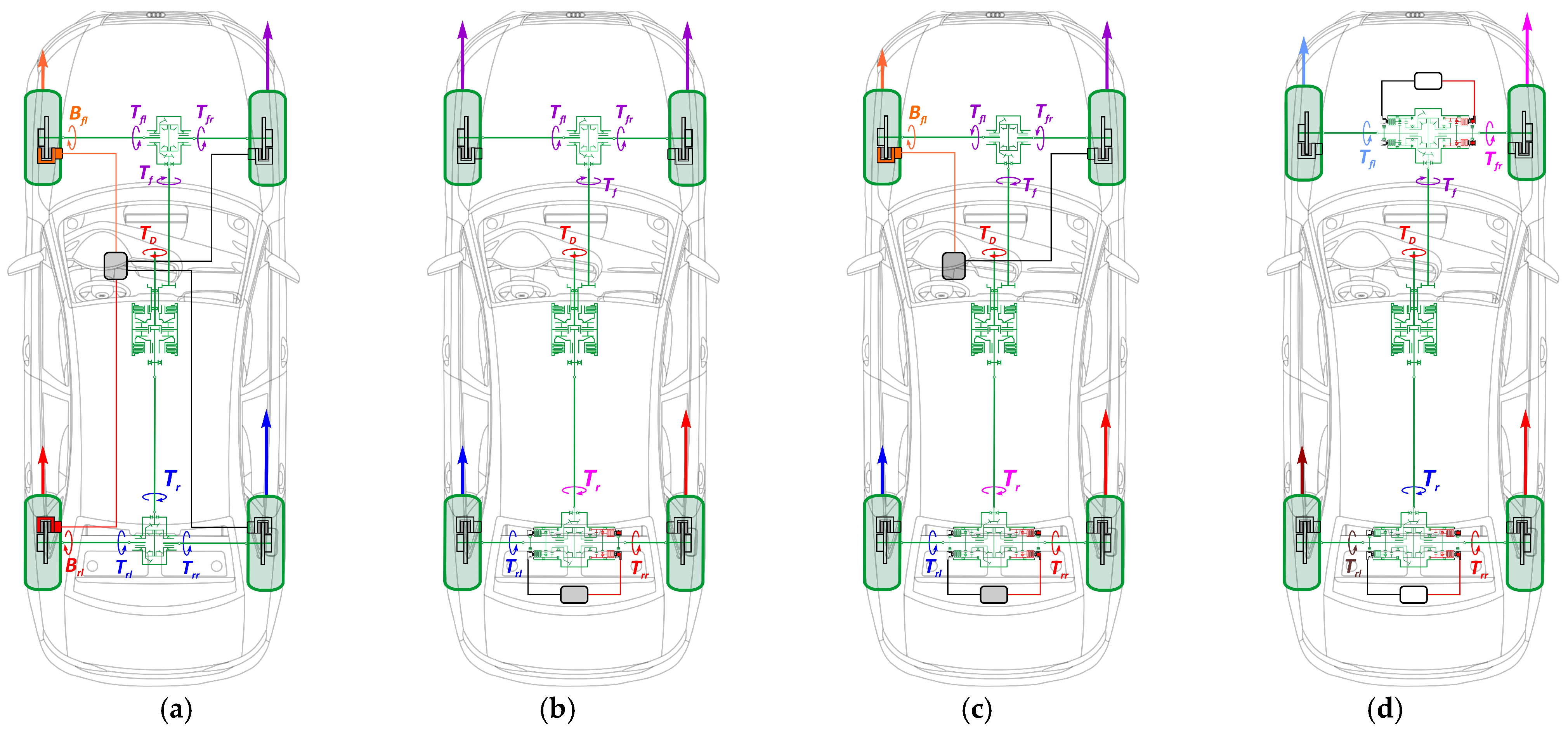
As a part of the objective of distributing the torque in the transmission of an all-wheel drive autonomous vehicle, four options can be implemented (Figure 4). Let us assume that the vehicle is equipped with a self-locking center differential (Audi Quattro), which does not require electronic control and distributes torques in a certain ratio depending on the output shafts’ resistances. Let us assume that at some motion moment, the longitudinal and lateral accelerations are positive, which causes a redistribution of vertical reactions to the rear axle and right side. We also make an important suggestion that the maximum friction coefficient φmax is the same for all wheels, that is, an unstable movement mode of any wheel occurs when the geometric sum of the longitudinal and lateral adhesion coefficients approaches the limit. Within the motion planning, we do not consider here the cases of control when the maximum possible adhesions on all wheels are different.
Let us consider the structural elements of transmissions in Figure 4 in more detail. The scheme in Figure 4a shows a variant of all-wheel drive with two symmetrical inter-wheel differentials, where the carriers’ drive torques are conditionally divided in half between the wheels’ semi-axles. In this scheme, to create an additional yaw moment stabilizing the vehicle steerability, it is necessary to slightly brake the wheels being in the worst adhesion conditions, that is, internal in this case. Due to the braking torques Bfl, Brl, it is possible to increase the drive moments of the axles and realize greater traction on the outer wheels.
The scheme in Figure 4b shows the case of using a sport differential (Tork Vectoring). Here, the front wheels are driven through a symmetrical differential, and the yaw moment is provided by redistributing the rear axle’s torques with a controlled (sport) differential. Since, for the case described, the outer rear wheel has more traction potential, by activating the hydraulic clutch larger torque is transferred to the wheel moving with the higher angular speed. At the same time, the torque on the inner wheel’s shaft is reduced. The difference in traction forces on the rear axle wheels produces a needed yaw moment.
The option in Figure 4c combines the rear axle’s sport differential and the front inner wheel’s brake activation. The variant in Figure 4d implements the full torque vectoring by using two inter-axle sport differentials. Structurally, this option is the most complex and expensive; however, obviously, it allows obtaining the best efficiency in torque redistribution.

2.4.2. Distribution Devices

Let us consider the transmission mechanisms ensuring the torque redistribution along with their dynamic and kinematic models.
Inter-axle (center) differential. Figure 5a shows the Audi Quattro self-locking differential belonging to the limited-sip (LSD) class. The different contact radii Rf, Rr of the output shafts’ crown gears (Figure 5b) give the initial asymmetry to the differential mechanism (DM) design. This leads to distributing the gearing torques with a ratio equal to 40/60 [24]. In normal conditions (both output shafts rotate with the same angular speed), the rear axle’s driving shaft transmits about 60% of the total torque, and the front axle −40%, correspondingly. Each crown gear has a friction clutch connecting it with the differential’s carrier. The relative sliding of friction elements generates moments that are redistributed according to the mechanism’s kinematic state. Thus, the output shaft’s torque may be reduced or increased. The clutch packs may be installed with precompression, stipulating the static friction torque by the pressing washers. With a decrease of one shaft’s resistance, its angular speed becomes greater than the carrier’s angular speed. The excessive power flow from an outrunning shaft returns to the carrier by the friction moment and increases the lagging shaft’s torque. A feature of this DM is the dynamic redistribution of friction moments due to the axial component of the gearing reaction. The greater the satellite’s force (Figure 5c), the greater the compression, and in turn, the greater the moment that can be passed by friction clutches.
The general kinematic relations for the asymmetric DM depicted in Figure 5, using the well-known Willis formula, may be reflected as follows
ω D = ω f + g f r ω r 1 + g f r
where ωD, ωf, and ωr = angular velocities of the differential carrier, front, and rear output shafts, respectively; and gfr = Rr/Rf = 60⁄40 = 3⁄2—algebraic ratio from the front drive axle to the rear drive axle.
The front and rear axles’ driving shafts’ angular speeds ωf, ωr can be estimated based on the symmetrical DM’s kinematic properties. Assuming that all wheels are rotating in approximately the same mode relative to the tires’ longitudinal slip, we can calculate with sufficient accuracy
ω f = i f ω f l + ω f r 2 = i f 2 v ζ 1 r e 1 + v ζ 3 r e 3 , ω r = i f ω r l + ω r r 2 = i f 2 v ζ 2 r e 2 + v ζ 4 r e 4
where ωfl, ωfr = angular speeds of the front left and right wheels, respectively, ωrl, ωrr = angular speeds of the rear left and right wheels, respectively, if = final gear ratio, v ζ j = longitudinal speed of the j-th wheel center in the wheel’s local coordinate system, and rej = wheel’s effective radius, j = [1, …, 4].
Thus, if during curvilinear motion, each wheel follows its trajectory without critical longitudinal slip, then, consequently, a certain ratio of output moments is established in the inter-axle (center) differential. This ratio is determined by the difference in angular speeds ωD, ωf, ωr. Note that the friction discs operate in an oily environment, which contributes to a smooth redistribution of output torques without the effects of sticking, and jamming, which are typical for cases close to dry friction. That is, to describe the frictional interaction, we may use an expression such as
μ F k = μ k tanh c k ω D ω k ,
where μFk = actual friction coefficient between friction pairs, μk = modulus of maximum friction coefficient, ck = intensity factor, k = f (front), and r (rear).
For each k = f, r shaft’s clutch, the dynamic friction torque Fkd is modeled as follows
F d k = n s P N k n F k R F k μ F k = n s P N k R k R F k R k n F k μ F k
where ns = number of satellites, PNk = axial gearing force, nFk = number of friction couples, Rk = average radius of side gear, and RFk = average friction radius.
Since the axial component PN of the gearing contact reaction, P depends neither on the direction of the shaft rotation nor on the direction of the tangential component PT, the friction moment’s dynamic part is written as follows
F d k = n s R k P T k tan α R F k R k n F k μ F k = M k η k , k = f , r
where PTk = tangential gearing force, α = gearing angle, Mk = side gear torque, and ηk = friction factor.
M k = n s R k P T k , η k = tan α R F k R k n F k μ F k
This DM also allows precompressing the friction clutches, which provides a static friction moment
F s k = P N 0 k R F k n F k μ F k
where PN0k = preliminary established axial compression force.
The preset friction moment can also be expressed in terms of the equivalent moment Mk0 on the side gears.
F s k = P N 0 k R k tan α tan α R F k R k n F k μ F k = P N 0 k R k tan α η k = M 0 k η k , k = f , r
Consider the distribution of moments without inertial forces for simplification. Let us introduce vector and matrix denotations
T = T f T r , M = M f M r , F d = F d f F d r , F s = F s f F s r , M 0 = M 0 f M 0 f , t D = 0.4 0.6 , E 2 = 1 0 0 1 , η = η f 0 0 η r , t M = t D t D
where vector tD is associated with initial torque redistribution.
The torques on the output shafts
T = M + F d + F s = E 2 + η M + η M 0
On the other hand, the drive torques on the side gears can be expressed in terms of the moment on the differential carrier TD
M = t D T D t M F d t M F s = t D T D t M η M t M η M 0
Whence
E 2 + t M η M = t D T D t M η M 0 , M = E 2 + t M η 1 t D T D t M η M 0
Substituting M in Equation (68), obtain
T = E 2 + η E 2 + t M η 1 t D T D t M η M 0 + η M 0
Denote
t E f = E 2 + η E 2 + t M η 1
Thus, if the kinematic distribution of the wheels’ angular speeds is given, the relations between the output shafts’ torques and the differential carrier’s torque
T = t E f t D T D + E 2 t E f t M η M 0
Note that the sensitivity of the moment distribution depends on the coefficient ck.
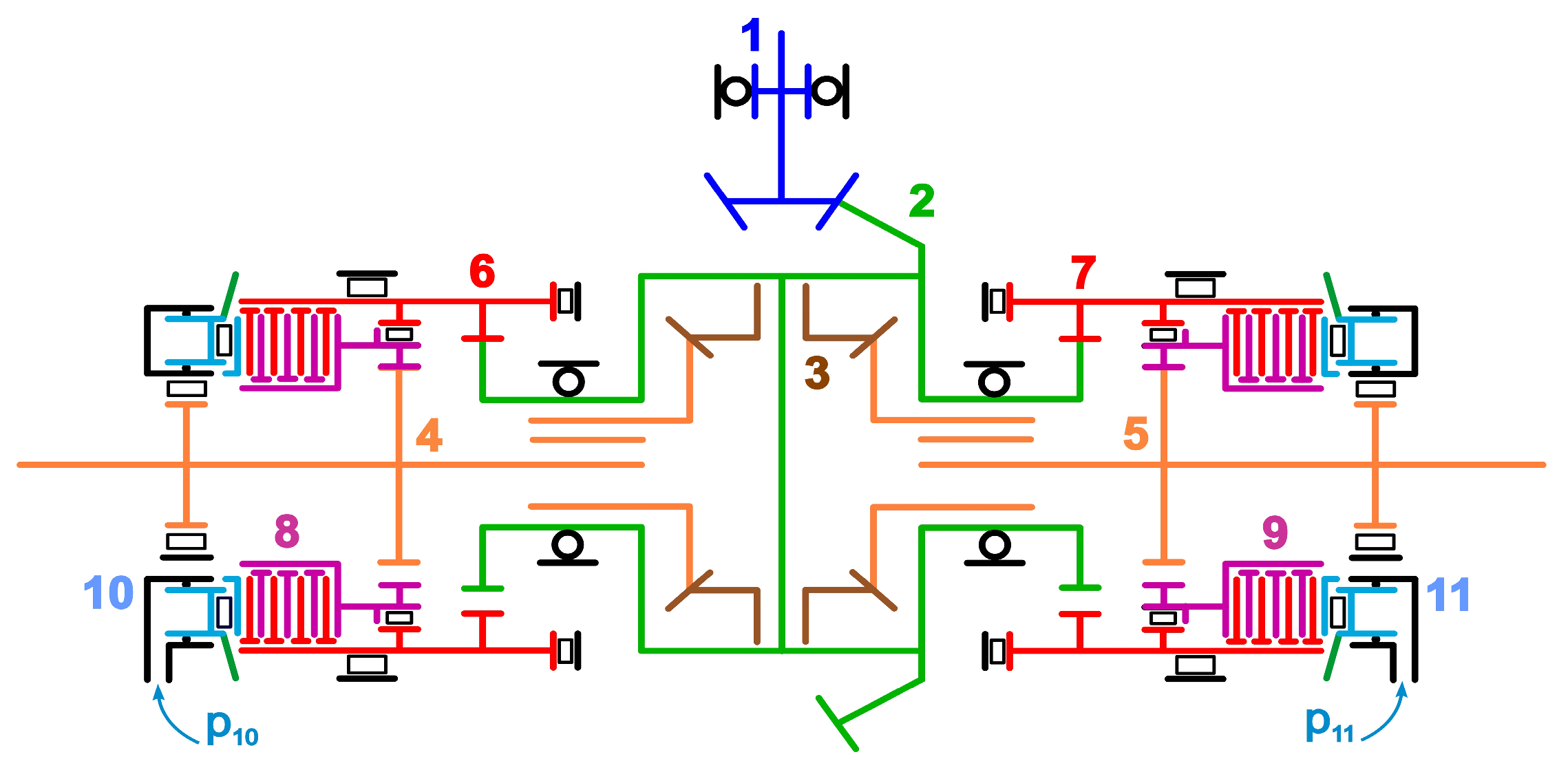
Inter-wheel Sport DM must ensure transmitting a larger torque to an outrunning axle, which causes additional cornering (yaw moment). Such a solution can be obtained using the design scheme and functioning of Audi Sport Differential shown in Figure 6.
The drive is carried out over the final gear pinion 1. The ring gear is rigidly connected to the differential carrier 2. Satellites 3, rotating around the axis fixed in the differential carrier, interact with side gears that drive the output axles 4 and 5 by the slots. The differential corps (carrier) has gear rims on the end sides for driving by internal gearing the coupling halves 6 and 7, in which rotational axes are, respectively, shifted relative to the carrier rotational axis. Using the frictional packs, the half-clutches 6 and 7 can drive the half-clutches 8 and 9, respectively, which are connected by internal gearing to the output shafts 4 and 5. Toroidal hydraulic cylinders 10 and 11 are installed from each side to act on the clutch packs using the pressure p10 and p11. Thus, by activating the required hydraulic cylinder, part of the carrier torque may be passed to the needed semi-axle using the frictional adhesion between the half-couplings over the two-step internal gearing (i28 = 0.8752, i26 = 1.2258, i84 = 0.714).
Since the Sport DM is formed based on a symmetrical one, it is possible to relate the moments on the output semi-axes Tl, Tr with the moment Td on the DM carrier and the moment ΔTlr of the friction clutch.
T l T r = t d T d Δ T l r , t d = 1 2 1 1 1 1 , T d Δ T l r = t s T l T r , t s = 1 1 1 1
Thus, the required friction clutch’s moment is equal to the difference of driving torques on the wheels’ semi-axles. Knowing the difference in the output shafts’ angular speeds, it is possible to calculate the required effect of the clutch drive.

2.4.3. Drivetrain Dynamics

Now, let us define the distribution and realization of traction forces on the wheels, considering the transmission type (Figure 4).
Since the drive of all wheels is realized by the same transmission, the drive torques can be linked to each other depending on the drive type. Let us consider options for using drives with torque vectoring (TV) between axles and wheels (Figure 4). Obviously, maximum vehicle controllability and stability are ensured when all the driving wheels work at the approximately same adhesion conditions. If we assume that each wheel realizes the same potential of longitudinal adhesion, then, consequently, all wheels will have a close potential of adhesion in the lateral direction. Let us search for distributing the transmission torques based on this ground.
Rewrite Equation (52) in the form regarding moments.
T j = R z j φ ζ j r w j + N j , N j = R z j f r j r w j + I w j a ζ j / r e j
where j = [1, 3] for the front axle, and j = [2, 4] for the rear axle.
Then, the ratios kf, kr of the moments on the front and rear axles’ wheels
R z 1 φ ζ 1 r w 1 R z 3 φ ζ 3 r w 3 = T 1 N 1 T 3 N 3 = k f , R z 2 φ ζ 2 r w 2 R z 4 φ ζ 4 r w 4 = T 2 N 2 T 4 N 4 = k r
As mentioned, we are trying to reach such a distribution of moments at which the adhesion potentials are the same and do not depend on the wheels’ loads. Then, optimally, φζ1 = φζ3 = φζf, which, after reduction, leads to equations
R z 1 r w 1 R z 3 r w 3 = k f , T 1 k f T 3 = N 1 k f N 3
Similarly, for the rear axle, based on the same principle that φζ2 = φζ4 = φζr,
R z 2 r w 2 R z 4 r w 4 = k r , T 2 k r T 4 = N 2 k r N 4
Note that with known distributions of speed and vertical reactions, the components Nj, as well as the coefficients kf, kr, can be obtained in advance.
Note that the wheels’ drive torques T1, T3 are generally not equivalent to the drive torques of the output shafts of the symmetrical differential Tfl = Tfr, nor are the torques T2, T4 with respect to the torques Trl = Trr.
Now, let us form a vector of driving moments for the cases using different DMs.
Case A. Front and rear symmetrical differentials share the torques Tf, Tr equally between the wheels’ semi-axles, i.e., Tfl = Tfr, Trl = Trr. The correction is fulfilled by activating the brake mechanisms, which stipulates the braking moments’ vector B. Then, the wheels’ torques will be related to semi-axle torques as follows
T w = t p T a B = t p t T i f T B
where tT is responsible for distributing the torque between the drive semi-axles, and tp is the matrix for permuting the Ta vector’s elements
T w = T 1 T 2 T 3 T 4 , T a = T f l T f r T r l T r r , t p = 1 0 0 0 0 0 1 0 0 1 0 0 0 0 0 1 ,
t T = 1 2 1 0 1 0 0 0 1 1 , B = B 1 B 2 B 3 B 4 , T = T f T r
At the same time, such a control vector B must be provided that satisfies the requirements of redistributing the moments from Equations (76) and (77) and minimizing the control in general.
T 1 k f T 3 = T f l B 1 k f T f r B 3 T 2 k r T 4 = T r l B 2 k r T r r B 4 B 1 B 3 = 0 ,   B 1 0 ,   B 3 0 B 2 B 4 = 0 ,   B 2 0 ,   B 4 0
Wheel torques in Equation (80) may be replaced according to Equations (76) and (77).
N 1 k f N 3 = T f l B 1 k f T f r B 3 N 2 k r N 4 = T r l B 2 k r T r r B 4
Then, the combination of additional linear and nonlinear conditions for braking torques will have the form
t A B B = t A t p T a N = t A t p t T i f T N
where
t A = 1 0 0 0 0 1 0 0 k f 0 0 0 0 k r 0 0 , t B = d i a g 0 0 B 1 B 2 , t A B = t A + t B
Note that we are only interested in positive values of the braking torques.
Substituting the expression from Equation (72) to Equation (78), we obtain
T w = t p t T i f t E f t D T D + E 2 t E f t M η M 0 B
Denote
k T D = i r w t p t T t E f t D i f , k M 0 = i r w t p t T E 2 t E f t M η i f
Substituting coefficients in Equation (52) yields
R ζ = i r w T w i r w N = k T D T D + k M 0 M 0 i r w N i r w B
Let us transform additional conditions
t A B B = t A t p t T i f t E f t D T D + E 2 t E f t M η M 0 t A N
Denote
k B T = t A t p t T t E f t D i f , k B M = t A t p t T E 2 t E f t M η i f
Substituting the expression from Equation (88) to Equation (87), we obtain additional conditions compactly
t A B B = k B T T D + k B M M 0 t A N
Thus, five unknowns are formed, such as torque TD and braking torques B.
Case B. The front symmetrical differential divides the torque Tf equally between the semi-axles without further correction, i.e., Tfl = Tfr = T1 = T3. The rear sport differential redistributes the drive torque Tr according to Equation (73). Then, the drive moments on the wheels will be related as follows
T f = T f l T f r = E 2 × 1 i f 2 T f , E 2 × 1 = 1 1 , T r = T r l T r r = t d T r i f Δ T r
Then, the vector of moments on the wheels’ drive shafts
T a = T f T r = 1 2 E 2 × 1 0 2 × 2 0 2 × 1 t d t f r i f T f i f T r Δ T r = t f r T t ,
where the matrix tfr = responsible for proportions of the distribution of moments, and
T t = i f T f i f T r Δ T r = i f T T r r T r l = i f T 1 k r T r r N 2 + k r N 4
Using Equation (92) and expanding Tt by components, we obtain
T a = t f r t T i f T + t a T a + t N N
where, considering E2 to be a 2 × 2 identity matrix,
t T = E 2 0 1 × 2 , t a = 0 0 0 0 0 0 0 0 0 0 0 1 k r , t N = 0 0 0 0 0 1 0 0 0 0 0 k r , N = N 1 N 2 N 3 N 4
Thus, the vector of semi-axles’ moments is expressed as
T a = E 4 t f r t a 1 t f r t T i f T + t N N = t e t f r t T i f T + t N N
Denote
t e = E 4 t f r t a 1
where vector tp ensures permuting the wheels’ numbering order, E4 = 4 × 4 identity matrix.
Then, the vector of wheels’ moments
T w = t p T a = t p t e t f r t T i f T + t N N
Substituting instead of T its expression from Equation (72) for the inter-axle differential drive, we obtain
T w = t p t e t f r t T i f t E f t D T D + E 2 t E f t M η M 0 + t N N   = t p t e t f r t T t E f t D i f T D + t p t e t f r t T E 2 t E f t M η i f M 0 + t p t e t f r t N N
Considering Equations (52) and (97), traction forces on the wheels can be calculated as follows
R ζ = i r w T w i r w N = i r w t p t e t f r t T t E f t D i f T D + i r w t p t e t f r t T E 2 t E f t M η i f M 0 + i r w t p t e t f r t N E 4 N
Denote
k T D = i r w t p t e t f r t T t E f t D i f , k M 0 = i r w t p t e t f r t T E 2 t E f t M η i f , k N = i r w t p t e t f r t N E 4
Then, in the compact form
R ζ = k T D T D + k M 0 M 0 + k N N
Case C. The front symmetrical differential divides the moment Tf equally between the semi-axles, i.e., Tfl = Tfr. The correction is made by activating the front brake mechanisms with braking torques B1, B3. The rear sport differential redistributes the drive torque Tr according to Equation (73). Then, the drive moments across the semi-axles will be related as follows
T w = t p T a t b B = t p t e t f r t T i f T + t N N t b B
T a = t e t f r t T i f T + t N N
By analogy with Equation (80)
T 1 k f T 3 = T f l B 1 k f T f r B 3 B 1 B 3 = 0 ,   B 1 0 ,   B 3 0 B 2 = B 4 = 0 , B = B 1 B 3 , t b = 1 0 0 0 0 0 1 0
Wheel moments in Equation (103) can be replaced according to Equation (76)
N 1 k f N 3 = T f l B 1 k f T f r B 3
Then, the combination of additional linear and nonlinear conditions for braking moments will have the form
t A B t b B = t A t p T a t A N = t A t p t e t f r t T i f T + t N N t A N
where
t A = 1 0 0 0 k f 0 0 0 , t B = 0 0 0 0 0 B 1 0 0 , t A B = t A + t B
Substituting the expression from Equation (72) to Equation (101), we obtain
T w = t p t e t f r t T i f t E f t D T D + E 2 t E f t M η M 0 + t N N t b B
Denote
i r w T w = i r w t p t e t f r t T t E f t D i f T D + i r w t p t e t f r t T E 2 t E f t M η i f M 0 + i r w t p t e t f r t N N i r w t b B , k T D = i r w t p t e t f r t T t E f t D i f , k M 0 = i r w t p t e t f r t T E 2 t E f t M η i f , k N = i r w t p t e t f r t N N E 4 , k B = i r w t b
Substituting the coefficients in Equation (52), we have
R ζ = i r w T w i r w N = k T D T D + k M 0 M 0 + k N N k B B
Denote
k B T = t A t p t e t f r t T t E f t D i f , k B M = t A t p t e t f r t T E 2 t E f t M η i f , k B N = t A t p t e t f r t N E 4
Then, the additional conditions
t A B t b B = k B T T D + k B M M 0 + k B N N
Case (d). In this scheme, the front and rear sport differentials redistribute the drive torques Tf, Tr following Equation (73). Then, the drive moments along all the semi-axles will be related as follows
T a = T f T r = t f r T t , t f r = t d 0 2 × 2 0 2 × 2 t d , T t = i f T f Δ T f i f T r Δ T r
where
T t = i f T f T f r T f l i f T r T r r T r l = i f T f 1 k f T f r N 1 + k f N 3 i f T r 1 k r T r r N 2 + k r N 4
Using Equation (113) and expanding Tt by components, we obtain
T a = t f r t T i f T + t a T a + t N N
where
t T = 1 0 0 0 0 1 0 0 , t a = 0 0 0 0 0 1 k f 0 0 0 0 0 0 0 0 0 1 k r , t N = 0 0 0 0 1 0 k f 0 0 0 0 0 0 1 0 k r
The subsequent technique corresponds to Equations (94)–(100).
Now, for drive variants in Figure 4, let us form systems of dynamics equations with additional conditions based on Section 2.2. Thus, each variant will have its own set of equations describing the traction dynamics and braking effect. Nevertheless, some equations describing the lateral forces will be common for all the schemes.
Case A. The system is nonlinear; therefore, we reformulate the equations of dynamics from Equation (54), substituting the vector Rζ from Equation (86).
E q 1 = k μ R μ k ζ i r w B + k ζ k T D T D + k ζ k M 0 M 0 k ζ i r w N k a a + k a d P a d = 0 3
The additional conditions for braking torques in the nonlinear form
E q 2 = t A B B k B T T D k B M M 0 + t A N = 0 4
Conditions for nonlinear tire’s lateral reactions based on Equation (41)
E q 3 = k R μ R μ = 0 2 , E q 4 = R μ f δ = 0 4
Then, the system of nonlinear equations and vector of variables are
E q = E q 1 E q 2 E q 3 E q 4 = 0 3 0 4 0 2 0 4 = 0 13 , x = R μ B T D δ
Cases B and D. These variants are distinguished by the generality of expressions and the absence of braking moments as unknowns. The equation of dynamics in the nonlinear form, given Equations (54) and (100).
E q 1 = k ζ k T D T D + k ζ k M 0 M 0 + k ζ k N N + k μ R μ + k a d P a d k a a = 0 3
In addition, we use Equation (117). Then, the system of nonlinear equations and vector of variables are
E q = E q 1 E q 3 E q 4 = 0 3 0 2 0 4 = 0 9 , x = R μ T D δ
Case C. The system is also nonlinear, therefore, we reformulate the equations of dynamic Equation (109), substituting the vector Rζ from Equation (54)
k μ R μ k ζ k B B + k ζ k T D T D + k ζ k M 0 M 0 + k ζ k N N k a a + k a d P a d = 0 3
Also, rewrite Equation (111) in the form
t A B t b B k B T T D k B M M 0 k B N N = 0 2
Then, the system of equations for unknown lateral reactions, front wheels’ braking moments and drive torque have a form similar to Equation (118). Note that the solution of nonlinear systems can be performed using the MATLAB lsqnonlin function.

3. Optimization

3.1. Generalized Approach to Speed Model

We proceed from the fact that some trajectory for the AV along a distance D has already been built. This question was extensively reflected in our previous studies. Using the general approach, let us compose models for obtaining the speed in finite elements (FE). The distance D may be divided on n FEs, each i-th of which is represented by the length Li and parameter ξ ∈ [0, 1]. Thus, the current linear space is x = ξLi. The basis functions Fξ are the form functions corresponding to the nodal degree of freedoms (DOFs) Qv. The number of nodal DOFs depends on the degree p of Lagrangian polynomial: d = (p + 1)/2. Then, any function y(x) within i-th FE may be expressed as follows:
l i = L i 0 L i d , L i = d i a g l i l i , y i x = y i Q v i , L i , ξ = Q v i T L i F ξ
We will use the second speed derivative as the basic model to reduce the polynomial extent p, the quantity of nodal unknowns, and speed up computations. Then, it can be written
d 2 V ζ i d x 2 = Q v i T L i F ξ , d 3 V ζ i d x 3 = Q v i T L i L i d F ξ d ξ
where nodal and FE parameters are
q v i = d 2 V ζ d x 2 i d 3 V ζ d x 3 i T , Q v i = q v i q v i + 1
Thus, d = 2 and we need the cubic Lagrangian polynomial to provide the smooth conjugating functions between all the segments. The first derivative of the longitudinal speed within i-th segment can be derived from the first integral
d V ζ i d x = d 2 V ζ i d x 2 d x + d V ζ i d x 0
where dVζi/dx(0) = integration constant defined from initial conditions.
The antiderivative is determined as
d 2 V ζ i d x 2 d x = Q v i T L i F ξ d x = Q v i T L i F ξ L i d ξ = Q v i T L i L i F ξ d ξ
The longitudinal speed Vζi in the i-th segment is found by repeating integration of Equation (126)
V ζ i = d 2 V ζ i d x 2 d x 2 + d V ζ i d x 0 x + V ζ i 0
where Vζi0 = integration constant corresponding to the initial speed for i-th segment.
Components of Equation (128) are found as follows
d 2 V ζ i d x 2 d x 2 = Q v i T L i L i 2 F ξ d ξ 2 , d V ζ i d x 0 x = L i d V ζ i d x 0 ξ

3.2. Optimization Technique

Minimization of an objective function S has the quadratic form and, considering nonlinear constraints, uses the SQP method. It can be written as
min q S q   subject   to   c e q q = 0 A e q q = b e q q L q q U , q = q 1 q n + 1 , q i = q d i 1 + 1 q d i 1 + d
where q = vector of nodal parameters; ceq(q) = vector function of nonlinear equality constraints; Aeq, beq = matrix and vector of linear equality constraints, respectively; qL, qU = lower and upper limits; and i  [1, n] = segment number.
The objective function may be a sum of integrals across all FEs. The integrals can be solved numerically using an N-point Gaussian quadrature scheme. Then, any integrand zi(x), replacing x = ξL, within an interval [xi−1, xi] can be evaluated as follows
x i 1 x i z i x d x = L i 0 1 z i Q v i , L i , ξ d ξ L i k = 1 N w k z i ξ ϑ k d e t J ϑ k
where wk = integration weight in the k-th point; ϑk = k-th point in the master–element coordinate system; J = Jacobian; k  [1, N]; and N = number of integration points.
For one-dimensional FE
ξ ϑ k = ξ 1 ξ 0 2 ϑ k + 1 + ξ 0 = 1 2 ϑ k + 1 , d e t J = ξ 1 ξ 0 2 = 1 2
Using vector designations,
ϑ = ϑ 1 ϑ N , w = w 1 w N , ξ = ξ 1 ξ N T , z i = z i , 1 z i , N T
we obtain a short expression for calculating the integral of Equation (71) along all n segments
i = 1 n L i 0 1 z i ξ d ξ 1 2 i = 1 n L i z i w = 1 2 L s z w
where Ls = vector of segment lengths; z = matrix of integrand values of n × N size; and
L s = L 1 L n T , z = z 1 z n = z 1 , 1 z 1 , N z n , 1 z n , N
Here, we use N = 6-point scheme enough for quality and performance.
Now, let us choose optimization criteria.
Longitudinal Speed Deviation relative to a preset upper-level VζU value along the path s.
I v = 0 s V ζ U V ζ 2 d s = 0 D V ζ U V ζ 2 s x d x = i = 1 n L i 0 1 z v i ξ d ξ
Denoting the integrand zvi(ξ), using a set of FE speed parameters Qvi from the model of Equation (124), a preset of the trajectory (curvature’s derivative) parameters Qti, and the approach of Equation (134), we have
z v i ξ = V ζ U V ζ Q v i , L i , ξ 2 s x Q t i , L i , ξ , z v i = z v i Q t i , Q v i , L i , ξ ϑ T , I v 1 2 L s z v w
where the trajectory scale factor is
s x = 1 + d y / d x 2
Third Derivative of Longitudinal Speed
I d 3 v = 0 s d 3 V ζ d x 3 2 d s = 0 D d 3 V ζ d x 3 2 s x d x = i = 1 n L i 0 1 z d 3 v i ξ d ξ
Denoting the integrand zd3vi(ξ) and considering the approach above, we obtain
z d 3 v i ξ = d 3 V ζ d x 3 Q v i , L i , ξ 2 s x Q t i , L i , ξ , z d 3 v i = z d 3 v i Q t i , Q v i , L i , ξ ϑ T , I d 3 v 1 2 L s z d 3 v w
Fourth Derivative of Longitudinal Speed
I d 4 v = 0 s d 4 V ζ d x 4 2 d s = 0 D d 4 V ζ d x 4 2 s x d x = i = 1 n L i 0 1 z d 4 v i ξ d ξ
Denoting the integrand zd4vi(ξ) and by analogy with the previous, we obtain
z d 4 v i ξ = d 4 V ζ d x 4 Q v i , L i , ξ 2 s x Q t i , L i , ξ , z d 4 v i = z d 4 v i Q t i , Q v i , L i , ξ ϑ T , I d 4 v 1 2 L s z d 4 v w
The speed’s objective function Sv is derived as the sum of the weighted criteria. Then, the following must be satisfied
S v = S v q v = W v T I v q v m i n
where qv = vector of speed’s second derivative’s nodal parameters (DOFs); Iv = vector of objective criteria integrals; and Wv = vector of weight factors.
W v = W v W d 3 v W d 4 v , I v = I v q v = I v q t , q v I d 3 v q t , q v I d 4 v q t , q v
where Wv, Wd3v, Wd4v = weight coefficients for quadratic velocity deviations and its third and fourth derivatives, respectively; and qt = vector of curvature’s (trajectory’s) derivative nodal parameters (DOFs).

4. Constraints

General Integral Approach to Nonlinear Equality Constraints. Since the kinematic, dynamic, and physical vehicle motion parameters have been formed, let us consider the integral technique of composing equality constraints. Suppose that smooth piecewise polynomial functions describe all the parameters based on the nodal DOFs of the speed and curvature derivatives. Since the numerical integration based on the Gaussian scheme is applied for optimization, the same scheme will be used to form restrictions. Assume that some parameter Ψ changes along the path s so that it does not exceed the upper ΨU and lower ΨL boundaries. Then, the sum of the areas between the upper limit ΨU and the function Ψ and between the lower limit ΨL and the function Ψ must be strictly equal to the area within boundaries. That is, for i-th FE and along the trajectory
x i 1 x i Ψ U Ψ L s x i d x = x i 1 x i Ψ U Ψ s x i d x + x i 1 x i Ψ Ψ L s x i d x
Integrals can be calculated numerically, for which we introduce the following denotations.
For integrals between bounds (UL), upper bound and function (UF), and function and lower bound (FL), we may denote:
z Ψ i U L ξ = Ψ U Ψ L s x i , z Ψ i U F ξ = Ψ U Ψ s x i , z Ψ i F L ξ = Ψ Ψ L s x i
Then, for the i-th path segment, using Equation (131), vectors of Equation (146) functions are represented as follows
z Ψ i k = z Ψ i k ξ ϑ T , k = U L ,   U F ,   F L
Combining all the segments, the integrals can be calculated numerically as
I Ψ k 1 2 L s z Ψ k w , k = U L ,   U F ,   F L
Thus, the requirement of nonlinear equality constraint along all the segments for a parameter Ψ, according to Equation (145) is expressed as follows
c Ψ = I Ψ U L I Ψ U F I Ψ F L = 0
Kinematic Parameters’ Constraints. Using this scheme above, we form a vector Ψk of nonlinear integral constraints for a series of kinematic parameters such as longitudinal speed, yaw rate, angular acceleration, and longitudinal jerk, where each j-th element corresponds to Ψkj.
Ψ k = V ζ ω ε j ζ , Ψ k U = V ζ U ω U ε U j ζ U , Ψ k L = V ζ L ω L ε L j ζ L , c k = c V ζ c ω c ε c j ζ = 0 4
where ΨkU, ΨkL = upper and lower limits of kinematic parameters, ck = vector of constraints corresponding to kinematic parameters.
Dynamic Parameters’ Constraints. The vector Ψd of dynamic parameters includes slip angles δ, tire lateral deformations Δμ, roll angle ψ, and longitudinal acceleration aζ as a function of speed. The maximum allowable roll angle at 0.4 g should not exceed 7°. For passenger cars, the recommended limit value is ψU = (10.8 − 4.3 B24/hg/2)°. We may accept 7.5°. Thus, introducing the limits ψL = −ψU. Let us use symmetrical limits.
A particular case is the limitation of the vehicle’s traction potential. The vehicle’s maximum acceleration depends on the speed and is due to design features. Thus, if the vehicle speed–acceleration characteristic is known, the condition must be met
V ζ i m i n V ζ i m a x a ζ U a ζ L d V ζ = V ζ i m i n V ζ i m a x a ζ U a ζ i d V ζ + V ζ i m i n V ζ i m a x a ζ i a ζ L d V ζ
where aζU, aζL = upper and lower limit values of acceleration potentially implemented by the vehicle.
The tire’s lateral deformation limits are ΔμL = −ΔμU. Combining the parameters, we obtain the vectors
Ψ d = δ Δ μ ψ a ζ , Ψ d U = δ U Δ μ U ψ U a ζ U , Ψ d L = δ L Δ μ L ψ L a ζ L , c d = c δ c Δ c ψ c a ζ = 0 10
Adhesion Constraints. Having calculated the necessary traction forces on the wheels according to Equation (54), including Equations (55) and (56), we determine the degree of using the longitudinal and lateral adhesions on each j-th wheel.
φ ζ j = R ζ j / R z j < φ m a x , φ μ j = R μ j / R z j
Then, the basic condition regarding the j-th wheel’s adhesion potential can be formed as follows
φ j = φ ζ j 2 + φ μ j 2 φ m a x
Using Equation (154), it is possible to impose physical restrictions on the conditions of all tire–road adhesions. Then
Ψ a = φ 1 φ 2 φ 3 φ 4 , Ψ a U = φ m a x 1 1 1 1 , Ψ a L = 0 0 0 0 , c a = c φ 1 c φ 2 c φ 3 c φ 4 = 0 4
Boundary Parameters’ Constraints. Another type of constraint determines the boundary conditions of kinematic parameters. Thus, one can require, for example, that the initial (0) and final (f) values of the predicted acceleration and jerk must correspond to preset constant values Aζ0(f) and Jζ0(f). That is,
Ψ b = a ζ 0 j ζ 0 a ζ f j ζ f , Ψ b 0 = A ζ 0 J ζ 0 0 0 , Ψ b f = 0 0 A ζ f J ζ f , c b = Ψ b Ψ b 0 Ψ b f = 0 4
The desired final speed may also be included.
Total restricting conditions. Thus, the complete sets of parameters, bounds, and nonlinear constraints are
Ψ = Ψ k Ψ d Ψ a Ψ b , Ψ U = Ψ k U Ψ d U Ψ a U Ψ b 0 , ψ L = Ψ k L Ψ d L Ψ a L Ψ b f , c e q = c k c d c a c b = 0 22

5. Simulation

Trajectory. As an example, consider planning a speed mode on a curvilinear section shown in Figure 7. Let us assume that the maneuver trajectory has already been determined by the inverse method described in our previous studies.
Before optimizing the speed mode, let us set the values of weight coefficients Wv in Equation (144) and limit values.
W v = 1 3 1 T
Speed derivative model limits
d V ζ d x U = 5.7   1 s , d 2 V ζ d x 2 U = 1   1 m s , d 3 V ζ d x 3 U = 0.1   1 m 2 s
Initial and limiting values of kinematic parameters
V ζ 0 = 60   k m h , V ζ U = 100   k m h , V ζ L = 50   k m h , a ζ U = φ m a x g   m s 2 , a ζ L = 0.5   m s 2 , a ζ 0 = a ζ f = 0   m s 2 , ω U = 0.5   r a d s , ε U = 3   r a d s 2 , j ζ U = 5   m s 3 , j ζ L = 2.5   m s 3 , j ζ 0 = j ζ f = 0   m s 3 δ U = 12   ° , Δ μ U = 2.5   c m , ψ U = 7.5   °
We use the data of Audi A4 3.2 FSI [24] to represent the AV. All the calculations are accomplished by using MATLAB tools [25].
Comparison of drive cases’ outputs. Figure 8 shows the results of output parameters for the various torque vectoring schemes corresponding to the variants (A, B, C, D) in Figure 4. Note that the same initial conditions and vehicle data are applied for all variants. Let us consider a case of road conditions that provide the maximum adhesion coefficient φmax = 0.5.
Longitudinal speed and acceleration. As seen in Figure 8a,b, all variants provide a smooth and similar shape increase in speed. The lowest peak values of speed and acceleration belong to variant (B) with single rear sport DM. Variants (A) and (D) show close results, which are explained by the same strategy of using the longitudinal adhesion potential for the same axle wheels. In this case, it does not matter in which way the redistribution of drive torques on the same axle’s wheels is achieved—due to internal or external moments relative to the semi-axles of the inter-wheel differential. Finally, the greatest speed and acceleration are achieved with variant (C), combining the rear sport DM and front brakes. This is because at the moment of vehicle acceleration, the inner front wheel is braked, which leads to an increase in resistance on its semi-axle with a subsequent torque raising on the opposite outer semi-axle. This results in growing the torque on the inter-axle differential’s output shafts. That is, this variant provides not only the torque distribution over the same axle wheels but partially over the axles too.
Jerk and roll angle. As seen in Figure 8c, longitudinal jerks differ in amplitude but do not exceed the specified limits, while simultaneously meeting the requirements of zero initial and final values. Obviously, with an increase in acceleration amplitude, the jerk also grows; nevertheless, the curves’ unambiguity and smoothness are ensured for all drive variants. This indicates a certain positive effect of the torque vectoring on the smoothness and stability of the curvilinear motion.
Figure 8d shows pseudo-roll angles reflecting the potential vehicle’s body roll due to predominantly centrifugal forces. Since the trajectory curvature determines the lateral acceleration, which is the same for all variants, the roll angles differ little and do not exceed the critical values.
Yaw rate and angular acceleration. As seen in Figure 8e,f, the curves of yaw rates and angular accelerations are almost the same for different drive control options. This is because the trajectory for all variants is the same and only the motion speed character stipulates the differences. Owing to the unprecedented smoothness and continuity of the angular acceleration functions, it is possible to successfully apply the inverse modeling approach, i.e., to evaluate force and dynamic parameters using the predefined kinematic ones. Note that the smoothness of all reference functions is one of the most important factors for the AV’s stable control.
Inter-axle (central) DM torques. Figure 8g shows the torques on the central differential’s carrier. As expected, the highest power costs correspond to variant (A), since the drive torques on the inner wheels are limited by the braking moments. That is, despite the high-quality regulation, this option requires excessive energy costs. The lowest energy consumption is provided by variant (B) with a rear sport DM, which requires almost 250 Nm less than in the case of variant (A). Variant (C) also ensures less torque than (A) and, nevertheless, more speed. Variant (D) is characterized by the lowest specific power costs regarding the speed mode since the torque redistribution is provided by internal and not external moments relative to the wheels’ driving semi-axles.
Figure 8h shows the distribution of torques between the vehicle axles by the variants. Note that the main difference in the values of the axles’ drive torques is observed in the first phase of acceleration since the effect of redistributing the vertical reactions is especially sensitive for the rear axle. As the steering angles and acceleration begin to diminish when the curvature decreases (about 35 m of the path), the rear tires’ kinematic radii instantly become smaller than the same radii of the front wheels. As a result, this leads to the temporal effect of equalizing the axles’ drive torques. Subsequently, owing to decreasing the influence of redistributing the vertical reactions and approaching the trajectory to a straight line, the ratio of torques becomes close to the mechanically preset in the inter-axle differential (i.e., 40/60).
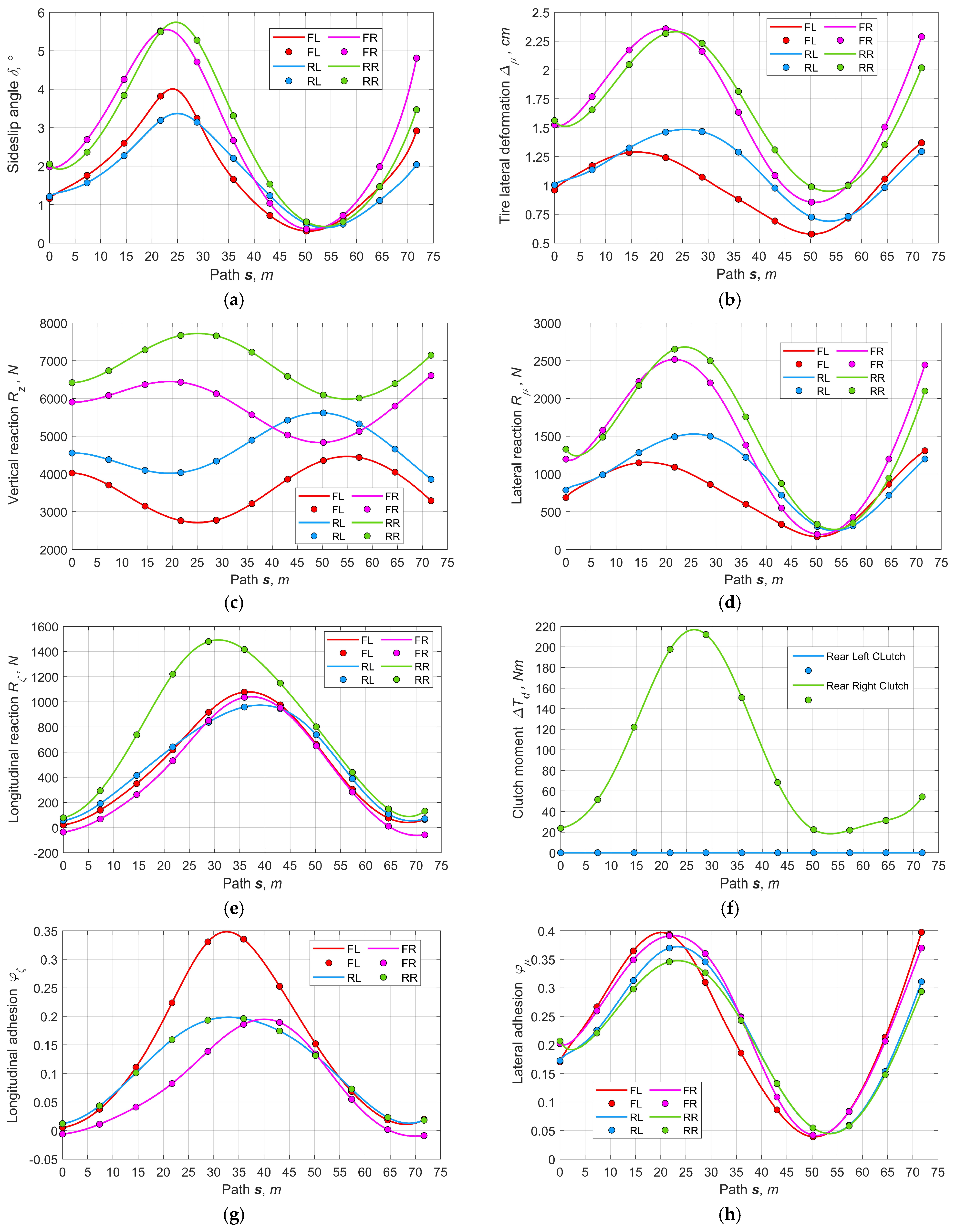
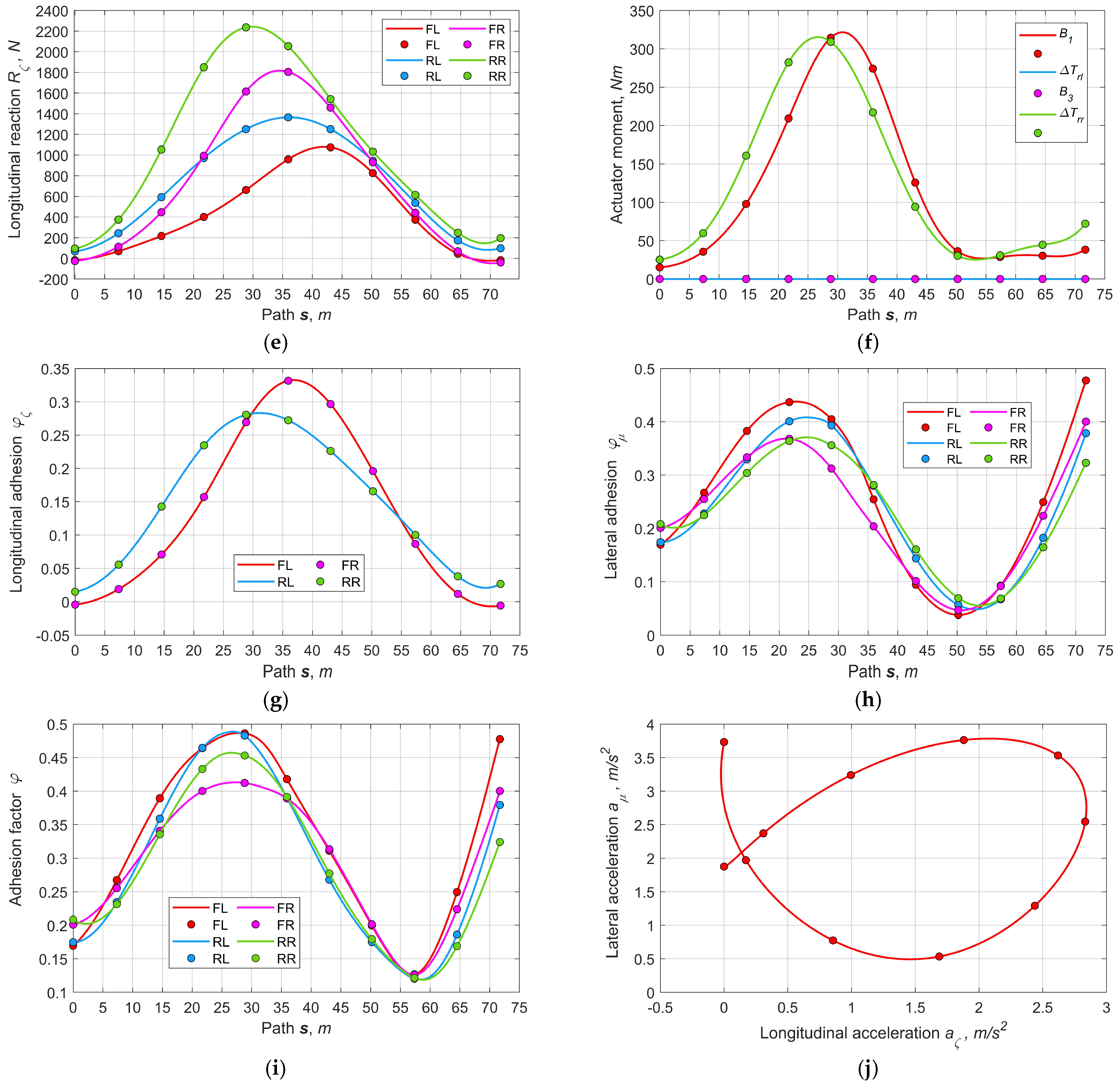
Case A. Figure 9 summarizes the results of optimizing the parameters for the variant by controlling the rear and front brakes. As seen (Figure 9a,b), the sideslip angles and the tires’ lateral deformations change smoothly and do not exceed the preset limits. The peak sideslip angles are reached by the front inner and rear outer wheels. In this case, the front inner wheel moves along the path with the greater curvature, and the rear outer wheel has the maximum vertical load (Figure 9c). The distribution of lateral forces (Figure 9d) is mostly proportional to the wheel loads. Due to individual adjustment, all longitudinal forces (Figure 9e) on the wheels are different. The braking moments are of greatest interest (Figure 9f).
As seen, the braking moments of the inner wheels change smoothly, and the front inner wheel’s braking moment is greater than that of the rear one. This is due to the need for withdrawing a larger moment from the front inner wheel, which is in worse adhesion conditions. At the same time, the braking moments of the outer wheels remain zero. Owing to the proposed strategy for distributing torques between the same axle wheels, the longitudinal adhesion potentials are pairwise the same for the wheels of the front and rear axles, respectively (Figure 9g). The lateral adhesion factor (Figure 9h) and total adhesion (Figure 9i) are represented by relatively narrow bunches of the common tendency curves. At the same time, none of the wheels violates the adhesion limit requirements. Figure 9j depicts the relation between the acceleration’s longitudinal and transversal components, showing continuity, smoothness, and good agreement with the trajectory curvature and the longitudinal speed’s derivatives as well.
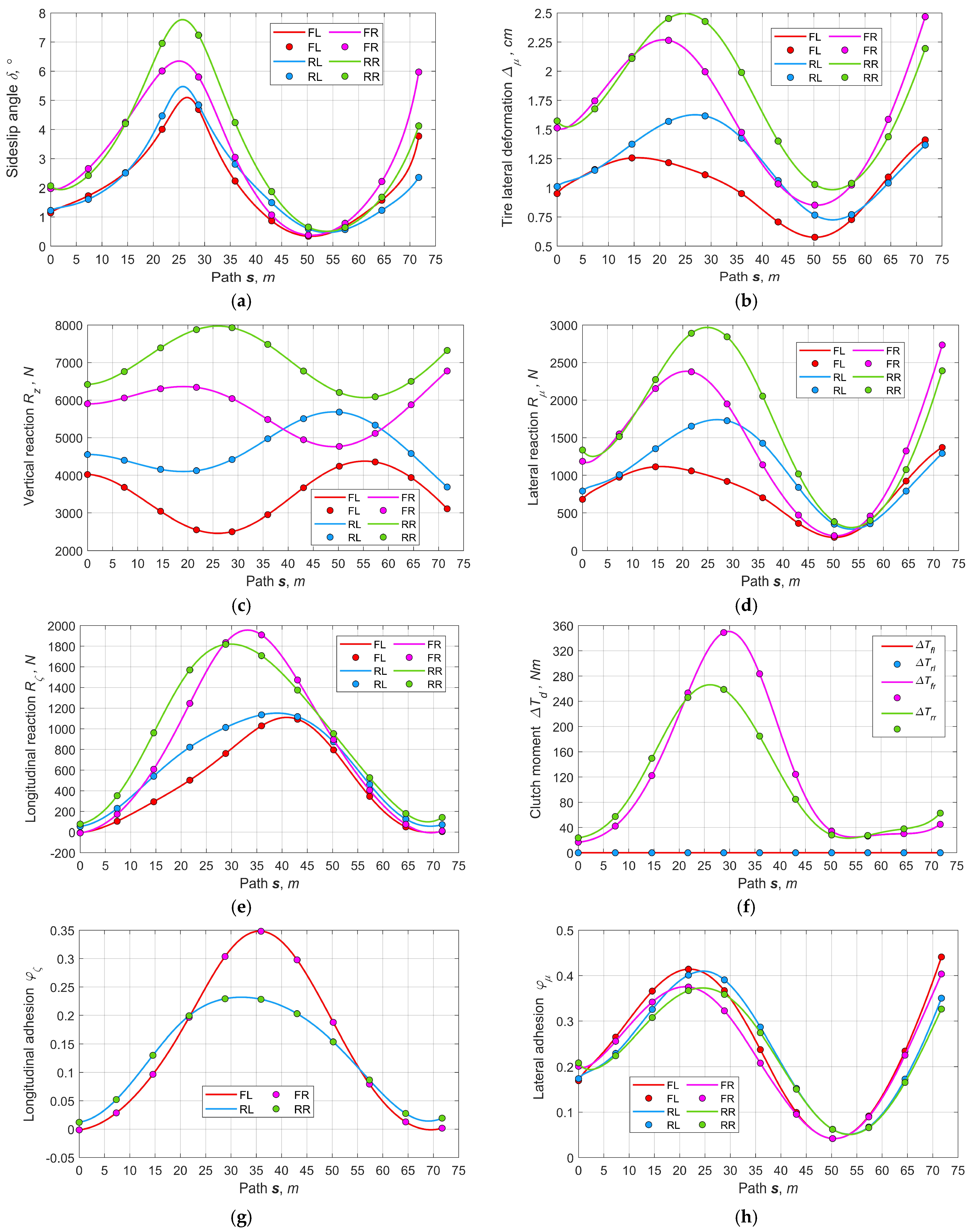
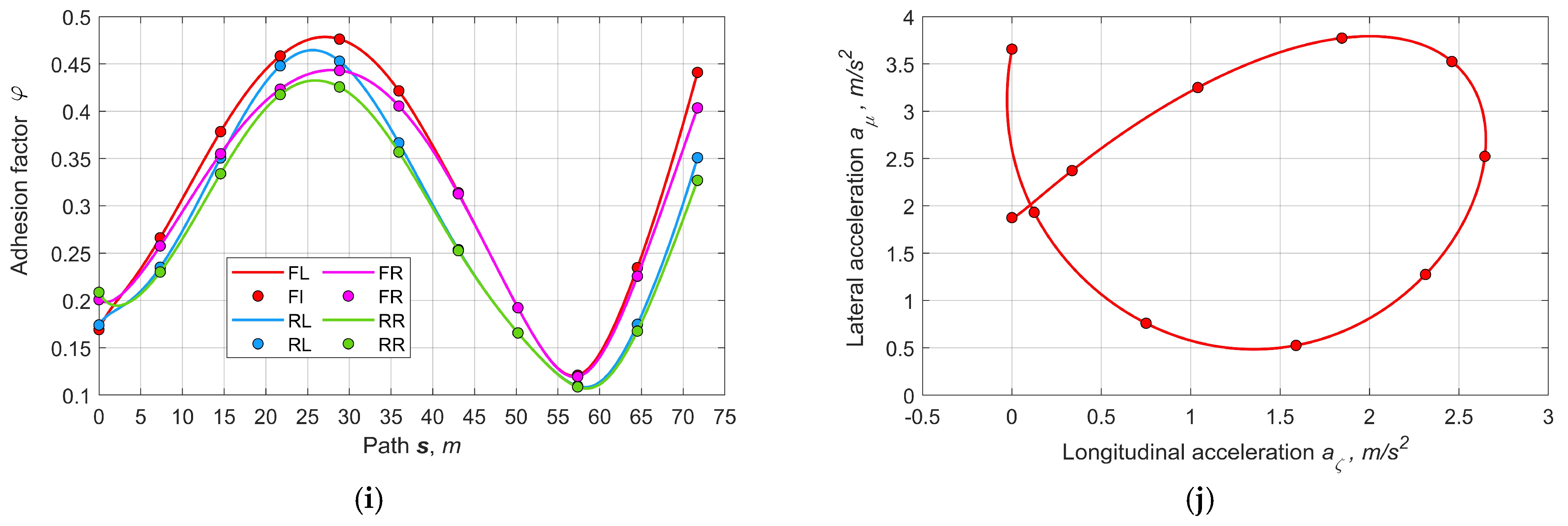
Case B. Figure 10 shows the results of optimizing parameters for the variant with a controlled rear sport DM. As seen (Figure 10a,b), the sideslip angles and the tires’ lateral deformations have the smallest values among all the variants since the speed is also the lowest. In Figure 10e reflecting the longitudinal reactions, as noted, the traction forces on the front wheels are almost coincident, which is explained by the equality of the drive torques on the semi-axles of the symmetric (open) front DM. Figure 10f depicts the internal moment of the rear sport DM, which is positive for the outer wheel’s clutch and zero for the inner wheel’s clutch. In Figure 10g, the rear wheels’ adhesion potentials are the same, unlike the front wheels. Thus, the adjustment possibilities are limited by the adhesion of the inner front wheel. Given the drive design at the specified road and initial conditions, this variant partially underuses the adhesion limit but provides good smoothness of the vehicle dynamics.
Case C. Figure 11 reflects the results of optimizing the parameters for the combined control variant with the rear sport DM and front brakes. As seen (Figure 11a,b), the sideslip angles and tires’ lateral deformations reach the largest values among all options since the speed is also the highest. In Figure 11e the wheels’ traction forces differ significantly in the maneuver’s first phase and converge in the second phase after decreasing the curvature. Figure 11f depicts the moments required for the rear sport DM’s clutches and front brakes. These moments are positive for the rear outer wheel’s clutch and front inner wheel’s brake, and they are zero for the rear inner wheel’s clutch and front outer wheel’s brake. In Figure 11g, the adhesion potentials of the front and rear wheels are pairwise coincident, which emphasizes the strategy’s effectiveness. Thus, the control possibilities are expanded and make it possible to bring the wheels to modes close to the limiting adhesion conditions if needed.
Case D. Figure 12 shows the results of optimizing the parameters for the variant with two controlled inter-wheel sport DMs. As seen (Figure 12a,b), the sideslip angles and tires’ lateral deformations are characterized by smoothness and their values do not exceed the corresponding limits. In Figure 12e the front wheels’ traction forces for this variant play the greatest role in comparison with other schemes, which has a positive effect on the vehicle steerability. Figure 12f depicts the internal moments of the sport DMs’ clutches, which are positive for the outer wheels’ clutches and zero for the inner wheels’ clutches. In Figure 12g, the front and rear wheels’ adhesion potentials are pairwise coincident. Thus, the possibilities of regulating motion stability and vehicle controllability are maximized.
Note that this drive variant is characterized by the highest cost despite the high efficiency and economy since there is no external resistance applied to the wheels’ semi-axle.
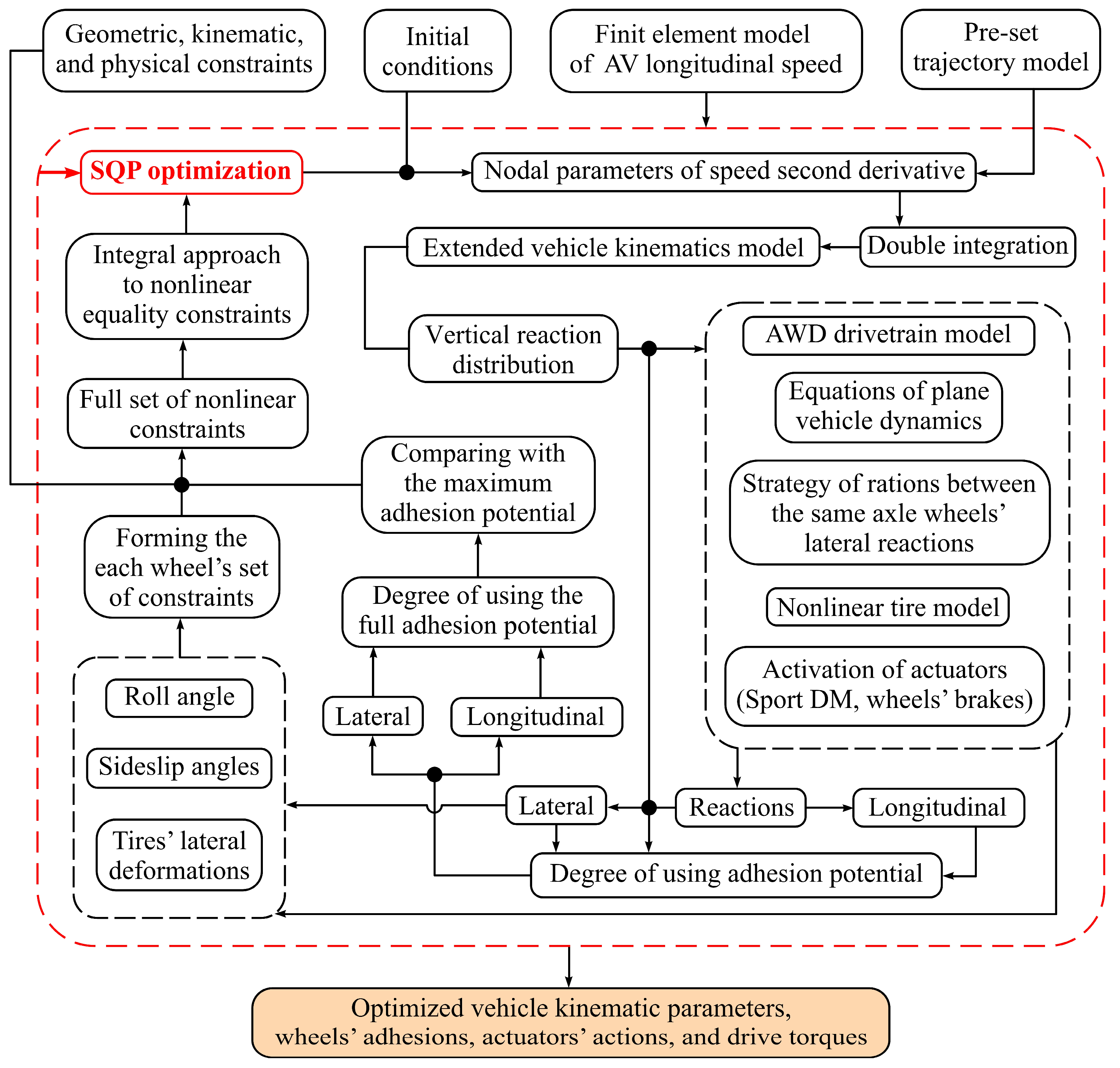
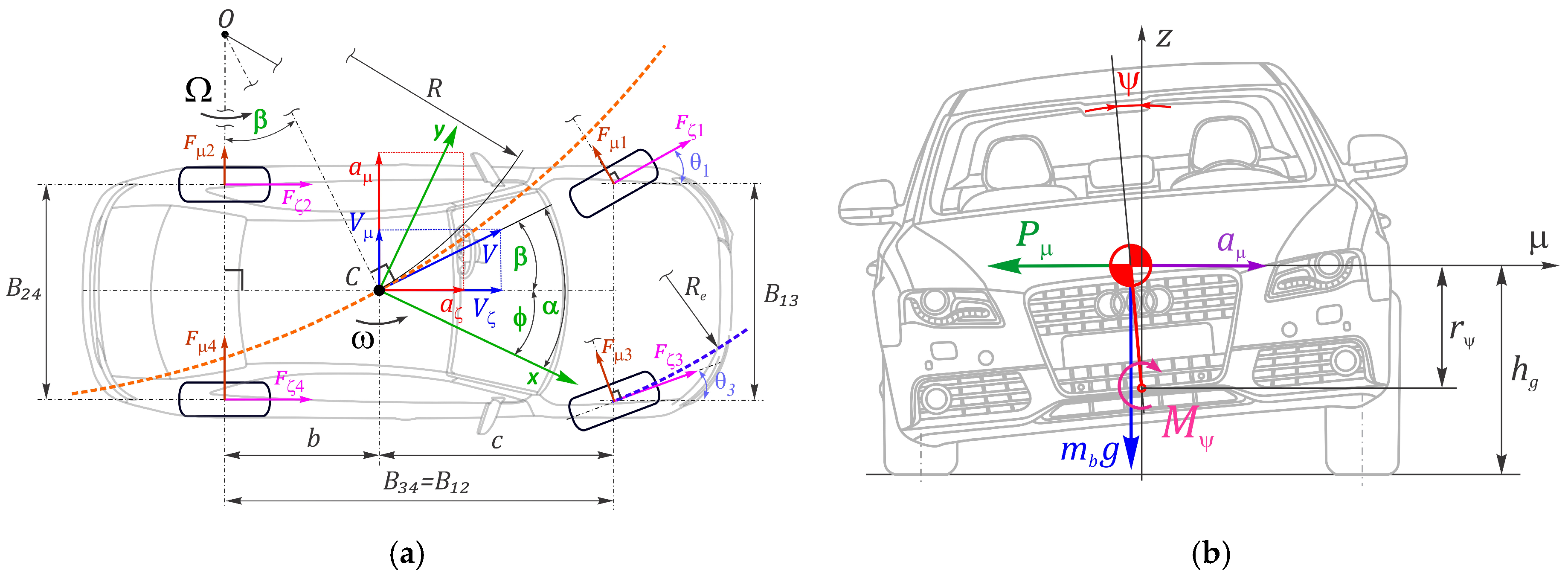
6. Conclusions

The main goal of this study is to improve the inverse modeling techniques for tasks on planning AV’s speed modes, considering the design features of the drivetrain structure. Based on the results, the following may be highlighted:
  • The proposed technique is highly efficient. The inverse approach provides stable, unambiguous functions for all kinematic, dynamic, and physical parameters, which are characterized by continuity and smoothness. In addition, the method’s performance is distinguished by its relative simplicity and versatility, confirmed by the successfully applied technique for predicting both trajectory and speed.
  • The vehicle’s motion dynamics significantly influences the formation of motion planning reference curves. This is facilitated by various dynamic and physical constraints built on the kinematic parameters to be optimized. The number of restrictions positively, in general, affects forecasts’ realism, considering the design features of vehicle’s drive, as well as the speed mode’s safety within the limits of vehicle capabilities.
  • Pseudo-parameters, such as sideslip, lateral tire deformation, and body roll, were used as extended criteria for motion safety, which allowed these physical parameters to be included in the nonlinear constraints of the AV kinematic model. Even though these parameters express equivalent values, their use increases the accuracy of forecasts and reduces the probability of critical regimes.
  • Parameters such as sideslip and tire lateral elasticity are the most sensitive to the curvilinear motion mode. The graphs show these parameters do not exceed the preset limits. However, the tangent angles of these curves at points close to the limit levels may be critical for the subsequent curves’ inflection at the next planning cycle. In this regard, the use of restricted derivatives for slip angles and tire lateral deformation may also be expedient.
  • The considered schemes of transmissions and control for distributing torques provide the effective capability of planning the actuators’ impact based on the AV kinematic model. At the same time, in accordance with the strategy of equal longitudinal adhesion potential of the same axle wheels, the curves’ smoothness of braking moments and friction clutches’ torques of sport DMs is ensured, which has a positive effect on maintaining the stability of both control and motion. The predetermined continuous kinematic parameters, such as yaw rate and angular acceleration make it possible to calculate with sufficient accuracy and smoothness a set of force parameters required for the vehicle model’s dynamic equilibrium.
  • Using a nonlinear tire model in the proposed approach had advantages and disadvantages. On the one hand, this leads to more accurate predictions of lateral forces, and on the other hand, due to the inevitable use of iterations in solving nonlinear equations, the optimization performance is worsened. Thus, regarding further improving the approach, a compromise between the modeling quality and the forecasting rapidity is needed, which may require the use of linearization followed by transiting from direct parameters to their increments with subsequent accumulation.

Author Contributions

Conceptualization, M.D. and S.M.E.; methodology, M.D.; software, M.D.; validation, M.D. and S.M.E.; formal analysis, S.M.E.; investigation, M.D.; resources, S.M.E.; data curation, M.D.; writing-original draft preparation, M.D.; writing-review and editing, S.M.E.; visualization, M.D.; supervision, S.M.E.; project administration, S.M.E.; funding acquisition, S.M.E. All authors have read and agreed to the published version of the manuscript.

Funding

This research is financially supported by the Natural Sciences and Engineering Research Council of Canada (grant No. RGPIN-2020-04667).

Institutional Review Board Statement

Not applicable.

Informed Consent Statement

Not applicable.

Data Availability Statement

Some or all data, models, or codes that support the findings of this study are available from the corresponding author upon reasonable request.

Conflicts of Interest

The authors declare no conflicts of interest.

References

  1. Vo, C.P.; Jeon, J.H. An Integrated Motion Planning Scheme for Safe Autonomous Vehicles in Highly Dynamic Environments. Electronics 2023, 12, 1566. [Google Scholar] [CrossRef]
  2. Ruof, J.; Mertens, M.B.; Buchholz, M.; Dietmayer, K. Real-Time Spatial Trajectory Planning for Urban Environments Using Dynamic Optimization. Robotics, Systems and Control. In Proceedings of the IEEE Intelligent Vehicles Symposium 2023, Anchorage, AK, USA, 4–7 June 2023. [Google Scholar] [CrossRef]
  3. Bianco, C.G.L.; Piazzi, A.; Romano, M. Velocity planning for autonomous vehicles. In Proceedings of the IEEE Intelligent Vehicles Symposium, Parma, Italy, 14–17 June 2004; pp. 413–418. [Google Scholar] [CrossRef]
  4. Kong, J.; Pfeiffer, M.; Schildbach, G.; Borrelli, F. Kinematic and dynamic vehicle models for autonomous driving control design. In Proceedings of the 2015 IEEE Intelligent Vehicles Symposium (IV), Seoul, Republic of Korea, 28 June–1 July 2015; pp. 1094–1099. [Google Scholar] [CrossRef]
  5. Mizushima, Y.; Okawa, I.; Nonaka, K. Model Predictive Control for Autonomous Vehicles with Speed Profile Shaping. IFAC-PapersOnLine 2019, 52, 31–36. [Google Scholar] [CrossRef]
  6. Piccinini, M.; Taddei, S.; Larcher, M.; Piazza, M.; Biral, F. A Physics-Driven Artificial Agent for Online Time-Optimal Vehicle Motion Planning and Control. IEEE Access 2023, 11, 46344–46372. [Google Scholar] [CrossRef]
  7. Altché, F.; Polack, P.; de La Fortelle, A. High-Speed Trajectory Planning for Autonomous Vehicles Using a Simple Dynamic Model. In Proceedings of the IEEE 20th International Conference on Intelligent Transportation, Yokohama, Japan, 16–19 October 2017. [Google Scholar]
  8. Ajanović, Z.; Regolin, E.; Shyrokau, B.; Ćatić, H.; Horn, M.; Ferrara, A. Search-Based Task and Motion Planning for Hybrid Systems: Agile Autonomous Vehicles. Eng. Appl. Artif. Intell. 2023, 121, 105893. [Google Scholar] [CrossRef]
  9. Cataffo, V.; Silano, G.; Iannelli, L.; Puig, V.; Glielmo, L. A Nonlinear Model Predictive Control Strategy for Autonomous Racing of Scale Vehicles. In Proceedings of the 2022 IEEE International Conference on Systems, Man, and Cybernetics (SMC), Prague, Czech Republic, 9–12 October 2022; pp. 100–105. [Google Scholar] [CrossRef]
  10. Rowold, M.; Ögretmen, L.; Kasolowsky, U.; Lohmann, B. Online Time-Optimal Trajectory Planning on Three-Dimensional Race Tracks, Robotics. In Proceedings of the 34th IEEE Intelligent Vehicles Symposium (IV), Anchorage, AK, USA, 4–7 June 2023. [Google Scholar] [CrossRef]
  11. Lamouik, I.; Yahyaouy, A.; Abdelouahed, S. Model Predictive Control for Full Autonomous Vehicle Overtaking. Transp. Res. Rec. J. Transp. Res. Board. 2023, 2677, 1193–1207. [Google Scholar] [CrossRef]
  12. Wu, H.; Long, X.; Lu, D. Trajectory Planning and Tracking for Four-Wheel Independent Drive Intelligent Vehicle Based on Model Predictive Control. SAE Int. J. Adv. Curr. Pract. Mobil. 2023, 5, 2471–2485. [Google Scholar] [CrossRef]
  13. Chen, Y.; Xin, R.; Cheng, J.; Zhang, Q.; Mei, X.; Liu, M.; Wang, L. Efficient Speed Planning for Autonomous Driving in Dynamic Environment with Interaction Point Model. IEEE Robot. Autom. Lett. 2022, 7, 11839–11846. [Google Scholar] [CrossRef]
  14. Zhou, S.; Tian, Y.; Walker, P.; Zhang, N. Impact of the tyre dynamics on autonomous vehicle path following control with front wheel steering and differential motor torque. IET Intell. Transp. Syst. 2023, 17, 1629–1648. [Google Scholar] [CrossRef]
  15. Xu, S.; Peng, H.; Song, Z.; Chen, K.; Tang, Y. Accurate and Smooth Speed Control for an Autonomous Vehicle. In Proceedings of the IEEE Intelligent Vehicles Symposium (IV), Changshu, China, 26–30 June 2018; pp. 1976–1982. [Google Scholar] [CrossRef]
  16. Kim, C.; Yoon, Y.; Kim, S.; Yoo, M.; Yi, K. Trajectory Planning and Control of Autonomous Vehicles for Static Vehicle Avoidance in Dynamic Traffic Environments. IEEE Access 2023, 11, 5772–5788. [Google Scholar] [CrossRef]
  17. Kim, C.; Yi, K.; Park, J. Hierarchical Motion Planning and Control Algorithm of Autonomous Racing Vehicles for Overtaking Maneuvers; SAE Technical Paper 2023-01-0698; SAE International: Pittsburgh, PA, USA, 2023. [Google Scholar] [CrossRef]
  18. Gao, J.; Claveau, F.; Pashkevich, A.; Chevrel, P. Real-time motion planning for an autonomous mobile robot with wheel-ground adhesion constraint. Adv. Robot. 2023, 37, 649–666. [Google Scholar] [CrossRef]
  19. Zulkifli, A.; Peeie, M.H.; Zakaria, M.A.; Ishak, M.I.; Shahrom, M.; Kujunni, B. Motion Planning and Tracking Trajectory of an Autonomous Emergency Braking Pedestrian (AEB-P) System Based on Different Brake Pad Friction Coefficients on Dry Road Surface. Int. J. Automot. Mech. Eng. 2022, 19, 10002–10013. [Google Scholar] [CrossRef]
  20. Jianshi, L.; Lou, J.; Li, Y.; Pan, S.; Xu, Y. Trajectory Tracking of Autonomous Vehicle Using Clothoid Curve. Appl. Sci. 2023, 13, 2733. [Google Scholar] [CrossRef]
  21. Grishkevich, A.I. Automobiles: Theory: Textbook for High Schools; Minsk High School: Minsk, Belarus, 1986; Volume 208, pp. 431–438. [Google Scholar]
  22. Krmela, J.; Beneš, L.; Krmelová, V. Tire Experiments on Static Adhesor for Obtaining the Radial Stiffness Value. Period. Polytech. Transp. Eng. 2014, 42, 125–129. [Google Scholar] [CrossRef]
  23. Pacejka, H.B. Tire and Vehicle Dynamics, 3rd ed.; Elsevier: Oxford, UK, 2012. [Google Scholar]
  24. Audi A4 Quatro Characteristics. 2023. Available online: http://www.automobile-catalog.com/car/2011/1187660/audi_a4_3_2_fsi_quattro_attraction_tiptronic.html (accessed on 19 January 2023).
  25. MATLAB R2022b. Available online: https://www.mathworks.com/ (accessed on 22 January 2023).
Figure 1. General scheme of the proposed approach.
Vehicles 06 00008 g001
Figure 2. Scheme of the 2.5D vehicle model: (a) ideal kinematics, (b) roll, (c) longitudinal, and (d) transversal dynamics.
Vehicles 06 00008 g002aVehicles 06 00008 g002b
Figure 3. Highlights of nonlinear tire slip: (a) effect of sideslip on side force, (b) effect of vertical load on slip coefficient, (c) slip inverse determination by the side force response.
Vehicles 06 00008 g003
Figure 4. Variants of wheel torque control individually: (a) using the same vehicle side’s brakes (Case A), (b) by driving the rear wheels through a sport differential (Case B), (c) by combining a rear sport differential and a front wheel’s brake (Case C), (d) by combining two sport differentials (Case D).
Vehicles 06 00008 g004
Figure 5. Asymmetric self-locking inter-axle DM with proportional friction moments: (a) design, (b) scheme, and (c) proportional action between satellites and crown gears.
Vehicles 06 00008 g005
Figure 6. Scheme of Audi Sport Differential.
Vehicles 06 00008 g006
Figure 7. Preplanned maneuver’s trajectory.
Vehicles 06 00008 g007
Figure 8. Comparison of kinematic and dynamic outputs by the drive variants (A, B, C, D): (a) speed, (b) longitudinal acceleration, (c) longitudinal jerk, (d) pseudo-roll angle, (e) yaw rate, (f) angular acceleration, (g) inter-axel differential carrier’s driving torque, (h) inter-axel differential’s front Tf and rear Tr output torques.
Vehicles 06 00008 g008
Figure 9. Basic output parameters for the variant of controlling the traction with wheels’ braking actuators (A): (a) sideslip pseudo-angles, (b) tires’ lateral pseudo-deformations, (c) vertical reactions, (d) lateral reactions, (e) longitudinal reactions, (f) wheels’ braking moments, (g) longitudinal adhesion factor, (h) lateral adhesion factor, (i) full adhesion factor, (j) relation between longitudinal and lateral accelerations.
Vehicles 06 00008 g009aVehicles 06 00008 g009b
Figure 10. Basic output parameters for the variant of controlling the traction with rear sport differential (B): (a) sideslip pseudo-angles, (b) tires’ lateral pseudo-deformations, (c) vertical reactions, (d) lateral reactions, (e) longitudinal reactions, (f) moments of rear SD’s clutches, (g) longitudinal adhesion factor, (h) lateral adhesion factor, (i) full adhesion factor, (j) relation between longitudinal and lateral accelerations.
Vehicles 06 00008 g010aVehicles 06 00008 g010b
Figure 11. Basic output parameters for the variant of combined controlling the traction with both the rear sport differential and the front brake actuators (C): (a) sideslip pseudo-angles, (b) tires’ lateral pseudo-deformations, (c) vertical reactions, (d) lateral reactions, (e) longitudinal reactions, (f) moments of rear SD’s clutches and front brakes, (g) longitudinal adhesion factor, (h) lateral adhesion factor, (i) full adhesion factor, (j) relation between longitudinal and lateral accelerations.
Vehicles 06 00008 g011aVehicles 06 00008 g011b
Figure 12. Basic output parameters for the variant of controlling the traction with rear sport differential (B): (a) sideslip pseudo-angles, (b) tires’ lateral pseudo-deformations, (c) vertical reactions, (d) lateral reactions, (e) longitudinal reactions, (f) moments of the front and rear SDs’ clutches, (g) longitudinal adhesion factor, (h) lateral adhesion factor, (i) full adhesion factor, (j) relation between longitudinal and lateral accelerations.
Vehicles 06 00008 g012aVehicles 06 00008 g012b
Disclaimer/Publisher’s Note: The statements, opinions and data contained in all publications are solely those of the individual author(s) and contributor(s) and not of MDPI and/or the editor(s). MDPI and/or the editor(s) disclaim responsibility for any injury to people or property resulting from any ideas, methods, instructions or products referred to in the content.