A Curb-Detection Network with a Tri-Plane BEV Encoder Module for Autonomous Delivery Vehicles

Abstract

Curb detection tasks play a crucial role in the perception of the autonomous driving environment for logistics vehicles. With the popularity of multi-modal sensors under the BEV (Bird’s Eye View) paradigm, curb detection tasks are increasingly being integrated into multi-task perception networks, achieving robust detection results. This paper modifies and integrates the tri-plane spatial feature representation method of the EG3D network from the field of 3D reconstruction into a BEV-based multi-modal sensor detection network, including LiDAR, pinhole cameras, and fisheye cameras. The system collects a total of 24,350 frames of data under real road conditions for experimentation, proving the effectiveness of the proposed method.

1. Introduction

With the rise of applications of AI in the field of autonomous deliveries, more and more specific subdivided tasks are emerging. With respect to autonomous logistics vehicles used in urban areas, the task of curb detection plays an important role not only for its safe navigation and precision in delivery, but also for autonomous parking.

In coping with the challenge of adverse weather and varying lighting conditions, LiDAR is usually a required item for sensor choice. Furthermore, the combination of telephoto cameras and fisheye cameras is beneficial for achieving both a 360-degree field of view and ensuring obstacle detection coverage. Early curb detection tasks were based on either pure vision [1,2] or pure mobile laser scanning [3] or LiDAR sensors [4]. As the requirements for environmental information in autonomous driving tasks have gradually increased, recent approaches have seen the emergence of deep learning-based, multi-modal detection methods. For instance, Deac [5] utilized a fisheye with LiDAR method, while Ma [6] employed a satellite imagery with LiDAR approach.

The combination of LiDAR and multi-view cameras in the BEV perspective is a popular paradigm in the industrial realm of autonomous driving perception. Curb detection methods based on this paradigm can also be more conveniently integrated into other road object detection and even prediction tasks, especially those involving the detection of lane lines, which are also road elements.

For these reasons, this paper analyzes relevant research on BEV feature representation methods (Section 2), proposes a deep learning network for multi-modal fusion curb detection using multiple fisheye cameras, pinhole cameras, and LiDAR (Section 3), validates the effectiveness of this method with real vehicle tests on a logistics vehicle (Section 4), and finally, analyzes the results (Section 5). The conclusions are summarized in Section 6.

2. Related Work

Due to the optical principles of lens imaging, object coordinates in the three-dimensional physical coordinate system often need to be mapped to the pixel plane through an appropriate camera projection model, while the reverse 2D-to-3D conversion process involves uncertainty. Moreover, to obtain a more accurate relationship for 3D-to-2D coordinate transformation, it is necessary to acquire a precise optical model of the camera through a rigorous camera calibration process. In these processes, fisheye cameras, because of their significant optical distortion, present additional challenges to obtaining more accurate 3D coordinate mapping relationships or extracting features through conventional image convolution methods. Consequently, in addition to traditional physical modeling methods [7], in recent years, many approaches based on deep learning, especially GAN-based [8] methods, have emerged for the distortion correction of fisheye camera images. Instead of estimating the heterogeneous distortion parameters, Liao et al. [9] constructed a distortion distribution map that intuitively indicates the global distortion features of a distorted image.

In the context of the BEV perception paradigm, it is a challenge to transform 2D features from multi-view camera images into 3D representations, contrasting with the natural three-dimensionality of LiDAR point clouds. The transformation process including geometric prior information, crucial for establishing directional accuracy, hinges on whether the optical model and camera extrinsic parameters are explicitly utilized for feature space transformation. Research in this area is broadly categorized into two main approaches. The first approach explicitly employs geometric prior information to project 2D features into the 3D space [10]. Conversely, the second approach begins with features in the BEV coordinates, facilitating interaction with 2D feature representations through 3D-to-2D feature map query modules derived mainly from transformer technology [11,12].

Furthermore, multi-view visual perception methods in BEV are transitioning from two-dimensional (front- or top-view) to three-dimensional (occupancy grid) representations. Occupancy grids partition the physical space into a voxel grid using a strategy that does not emphasize object classification but is dedicated to detecting whether there are obstacles in the road space.

Feature extraction in the field of 3D reconstruction typically involves optimizing a differentiable 3D spatial feature representation using multi-view images [13,14]. The seminal work NeRF [15] implicitly represents scenes using positional encoding and fully connected layers, which is relatively computationally expensive; explicit discrete voxel grid representation methods [16] present a significant challenge to memory space, whereas local implicit representations [17] and hybrid explicit–-implicit representations [18] adopt a compromise approach, achieving a favorable balance between the above-mentioned two.

This paper is inspired by the spatial feature representation of the generator in the EG3D [19] network within the field of 3D reconstruction and modifies its tri-plane feature representation method to the feature space transformation in BEV in the task of curb detection.

Furthermore, for the spatial interaction and feature fusion of multi-view camera images, we utilize the attention mechanism, which is widely employed in transformer-derivative networks, to establish the interaction between multi-view cameras. Moreover, to reduce the computational cost of queries, we integrate the mechanism of deformable attention [20] into the feature fusion method.

3. Methodology

To complete the projection transformation from 2D image space to 3D BEV perspective, inspired by the generator in the EG3D network, this paper designs a “modified tri-plane BEV-encoder” to accomplish the BEV feature encoding task for multi-view camera information. This module is then applied to the curb detection network of a logistic vehicle. Section 3.1 introduces the structure of the “modified tri-plane BEV-encoder”, and Section 3.2 explains how the images from fisheye cameras are rectified. Section 3.3 discusses the construction of the multi-modal sensor curb detection network.

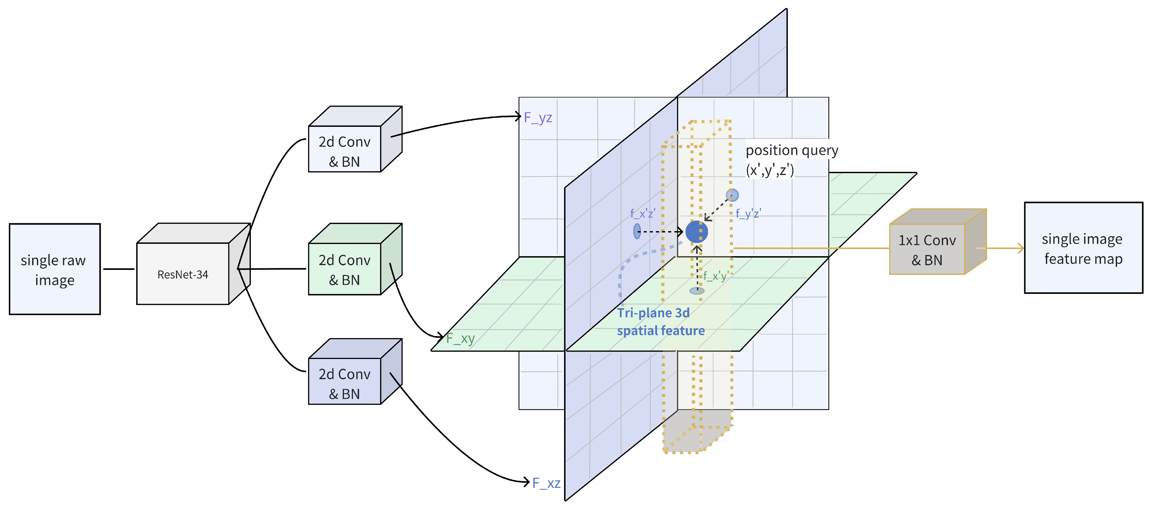
3.1. Modified Tri-Plane BEV-Encoder

Figure 1 shows the schematic diagram of the “modified tri-plane BEV-encoder” structure exemplified by data from a single camera. After preprocessing the original image, features are extracted using ResNet-34 and then passed through three different modules composed of 2D convolutions and BN (Batch Normalization) layers. These modules split and map the feature channels extracted by the backbone into three feature planes (namely $F_{xy}$, $F_{yz}$, $F_{xz}$ planes), thereby dividing the 3D space into a corresponding number of voxels using the grid of the three planes.

Unlike the direct voxel representation method, where the memory occupied by the features grows cubically with the width of the feature map, to save memory consumption, this paper employs the tri-plane method of spatial feature representation [19]. The blue sphere represents the “tri-plane” feature at a certain spatial position coordinate ($x^{\prime }$, $y^{\prime }$, $z^{\prime }$) in the 3D voxel space. Its position coordinates are projected onto the $F_{xy}$, $F_{yz}$, $F_{xz}$ planes, and the features on the three planes are, respectively, indexed as $f_{x^{\prime }{y}^{\prime }}$, $f_{y^{\prime }{z}^{\prime }}$, $f_{x^{\prime }{z}^{\prime }}$. By adding these features together, we obtain the “tri-plane 3D spatial feature”. Subsequently, the spatial features located on the same “pillar” in the BEV perspective are encoded using 1D convolution and a BN (Batch-Normalization) layer, thus obtaining the output feature map.

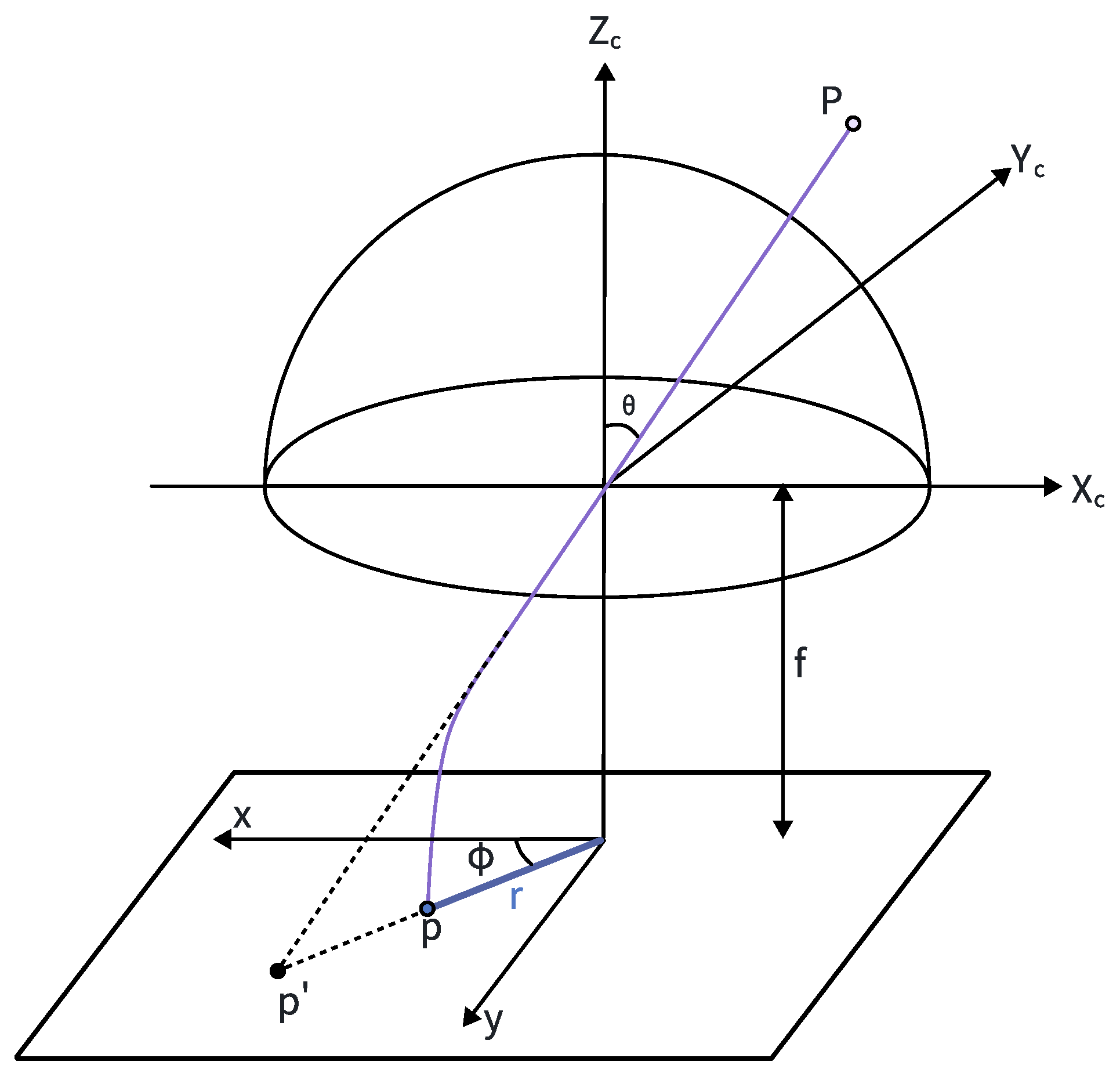
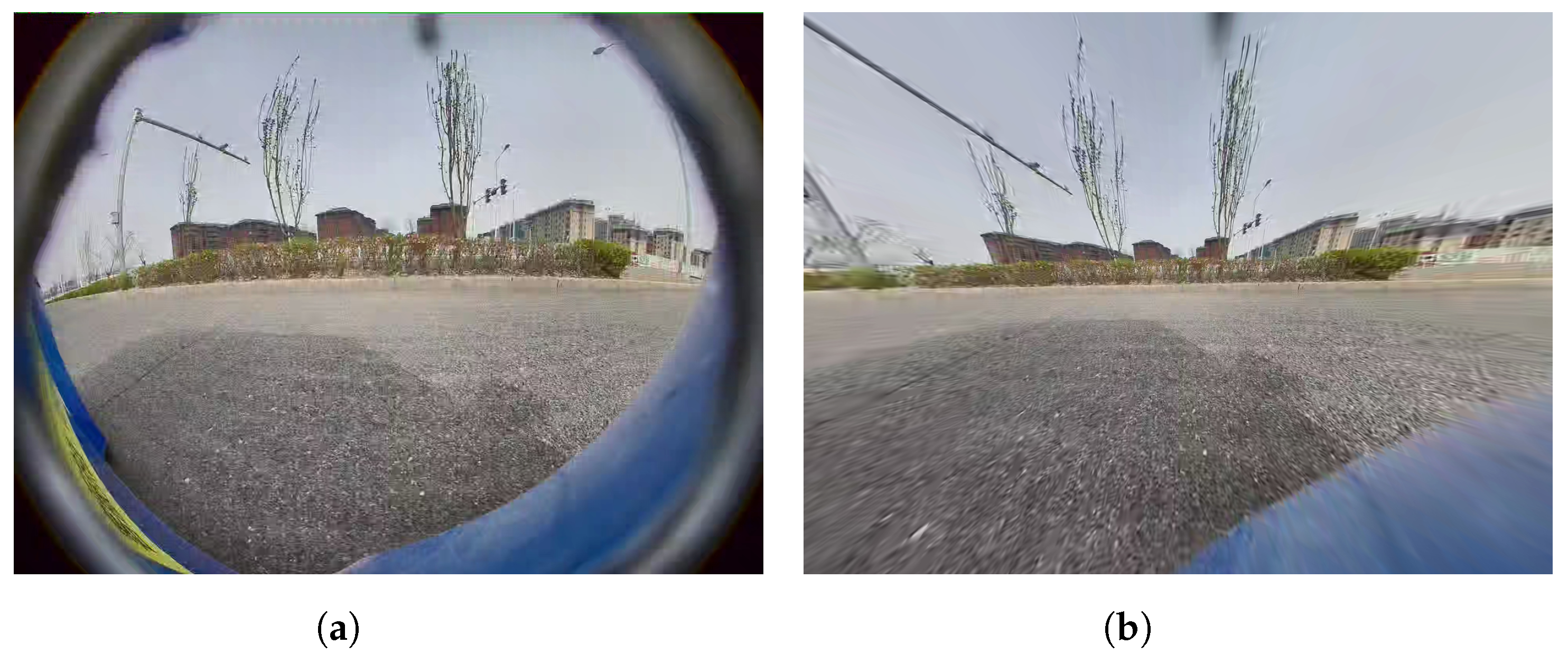
3.2. A Fisheye-Camera Rectification Module

The perspective projection of a general pinhole camera can be described by Equation (1), where f represents the focal length of lens, $\theta$ is the angle between the ray from the camera’s principal axis to the point P in the real word and the principal axis itself, and r refers to the distance between the image point and the principal point.

$$r=ftan\theta ,$$

(1)

Due to the unique distortion characteristics of fisheye cameras, however, distinct models for projection are employed, such as orthogonal projection (Equation (2)), equidistant projection (Equation (3)), etc.

$$r=fsin\left(\theta \right)$$

(2)

$$r=f\theta$$

(3)

To obtain a universal expression, in the research by Kannala and Brandt [21], a general radially symmetric model (Equation (4)) is used to represent the perspective projection model of traditional, wide-angle, and fisheye lens cameras, and a corresponding calibration method is provided.

$$r\left(\theta \right)=k_1\theta +k_2{\theta }^3+k_3{\theta }^5+k_4{\theta }^7+k_5{\theta }^9+\dots$$

(4)

Here, as is shown in Figure 2, $r\left(\varphi \right)$ represents the radial distance from a point on the image plane to the principal point, and $k_1$, $k_2$, and … are the model parameters.

This model has been extensively applied in the industry, such as the fisheye camera model implemented in OpenCV [22]. By employing higher-order polynomials, the model can approximate real lens distortions with high accuracy; however, to balance the cost of calibration, employing a second-order polynomial is a common practice. Therefore, this paper employs the following simplified model, which is implemented by OpenCV [23], to correct the distortion from fisheye cameras in the pixel coordinate:

$$\left[\begin{array}{c}{x}^{\prime }\\ y^{\prime }\end{array}\right]=\left(1+K_1{r}_d^2+K_2{r}_d^4\right)\left[\begin{array}{c}x\\ y\end{array}\right]+\left[\begin{array}{c}2p_{1}xy+p_2\left(r_d^2+2x^2\right)\\ 2p_1\left(r_d^2+2y^2\right)+2p_{2}xy\end{array}\right]$$

(5)

$$r_d^2=x^2+y^2$$

(6)

where $p_1$, $p_2$ are tangential distortion coefficients and $K_1$, $K_2$ are radial distortion coefficients.

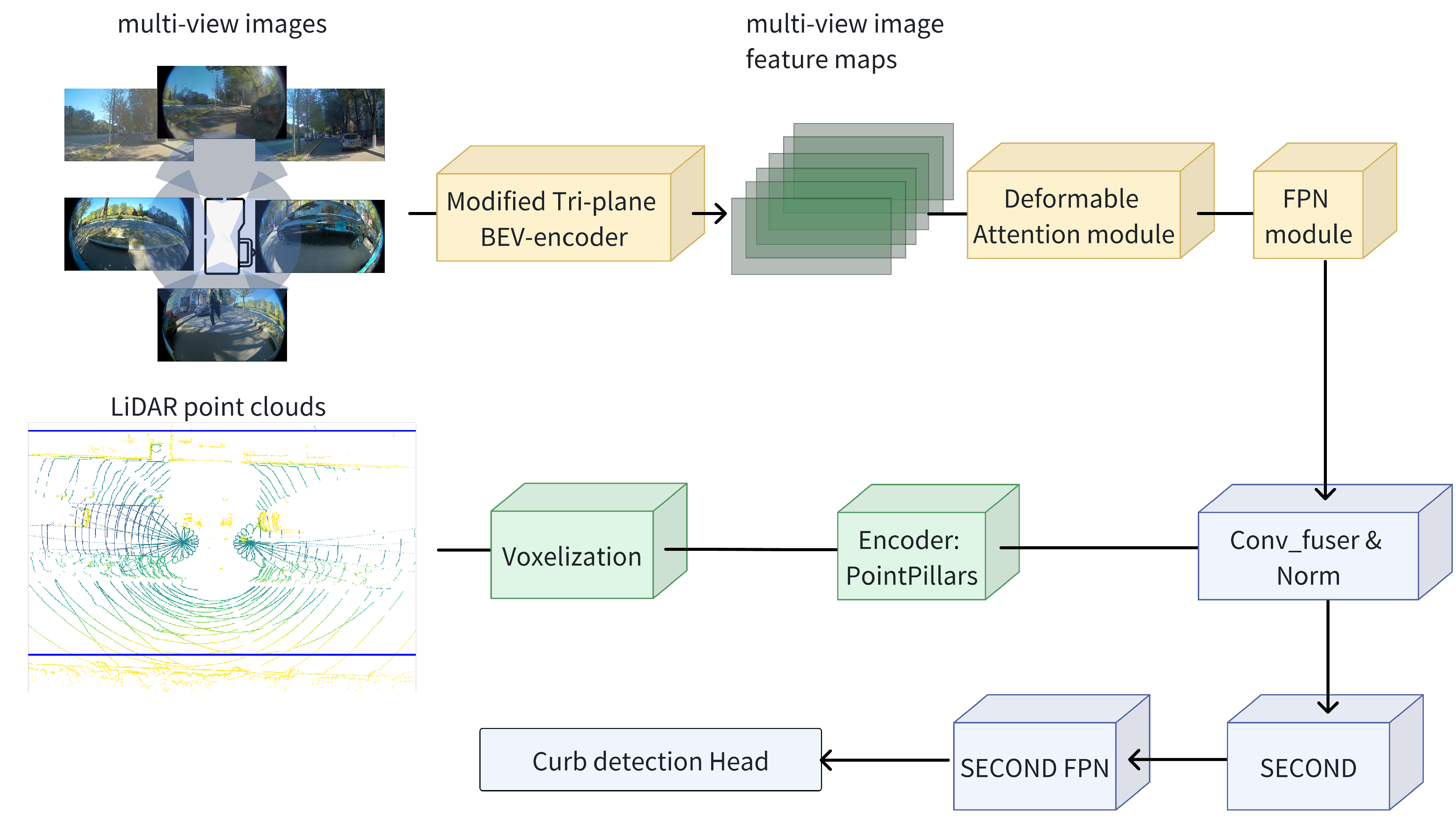
3.3. A Curb-Detection Algorithm Using LiDAR–Camera Fusion with a Tri-Plane BEV-Encoder

To fuse multi-modal sensor data (to fuse multi-modal sensor data from a setup comprising five LiDAR and six cameras, including both pinhole and fisheye types), this paper designs a curb detection network structure as shown in Figure 3 and implements it using the MMDetection [24] framework.

For the camera branch: after preprocessing and data augmentation, the original images are fed into the “modified tri-plane BEV-encoder” module described in Section 3.2 to obtain multi-camera feature maps. These are then processed with deformable attention to extract and fuse spatial information of interest from multiple viewpoints in the BEV perspective. Subsequently, multi-scale features are fused through the FPN (Feature Pyramid Network) module.

For the LiDAR branch, data outside the region of interest is filtered out. The point cloud is voxelized in the manner of PointPillars and input into the PointPillarsEncoder [25], which consists of the PillarFeatureNet as points voxel encoder and the PointPillarsScatter as points middle encoder, to obtain the point cloud feature map in the BEV perspective.

Then, the data from the two modalities are fused using convolutional methods and are input into the decoder composed of the SECOND backbone and SECOND FPN for curb detection [26].

The curb detection head is composed of three branches. Bilinear interpolation is applied to the ground truth annotations of curbs as needed, allowing for loss calculation of the following three branches by querying the relationship between the BEV grid and the actual 3D space coordinates:

• Semantic Segmentation Branch: a binary classification semantic segmentation branch for predicting whether each BEV grid cell belongs to the lane line;
• Instance Segmentation Branch: used to distinguish between different lane lines instances;
• Position Offset Branch: predicts the minimum distance of lane line instances from the center of the BEV grid cells, serving as the position offset loss for curb detection in order to enhance detection accuracy. The output channel number is 2, corresponding to the offset in the x and y directions.

4. Experiments

4.1. Dataset Setup

The experimental logistics vehicle was equipped with six cameras and five LiDAR sensors: one telephoto pinhole camera and one wide-angle pinhole camera were mounted in the front-view direction, while four fisheye cameras were installed at the front, back, left, and right views, respectively; there are two livox LiDARs at the front and the back view; one 16-line LiDAR on both the left and right sides; and a 32-line LiDAR mounted on the top (as shown in Figure 3).

The logistics vehicle collected a total of 24,350 frames of data in urban areas, including conditions during clear weather, rainy weather, and nighttime driving.

For the curb instance annotation, a set of key-points was used, selecting sufficient key-points on the curb to represent its shape, and these points were annotated with their spatial two-dimensional Cartesian coordinates in the vehicle’s ego-coordinate system (In the vehicle’s coordinate system, the direction in front of the vehicle is defined as the positive direction of the x-axis, and the left side of the vehicle is defined as the positive direction of the y-axis, with the z-axis direction being disregarded).

4.2. Fisheye Camera Rectification

To test whether correcting the distortion of fisheye cameras affects feature extraction, this paper employs the Kannala–Brandt model [21] to correct the original images from fisheye cameras before using them as the initial input for network training, as is shown in Figure 4. It also compares the impact on detection performance with and without the fisheye camera distortion correction step.

4.3. Comparison with Existing Image-to-BEV Feature Projection Method

As outlined in Section 2, establishing a relationship between image features and BEV-space features based on prior knowledge such as the physical rotation and translation relationships as well as the optical model of camera imaging is an intuitive approach. This method, by leveraging prior information instead of encoding features through hidden layers in deep learning network, conserves a significant number of learnable parameters. Consequently, it offers substantial advantages in training and inference speed due to the reduced computational complexity.

Drawing from the foundational concepts of M²BEV [27], fast-BEV [28] enhances the view transformation process introduced by M²BEV. It adopts a strategy similar to the edge-3D’s use of a look-up table to associate tri-plane features with voxel features in the BEV space (Equation (7)), where the 3D voxel projection technique is predicated on the hypothesis that the depth distribution along a camera ray is uniform. That implies that each voxel intersected by the same ray possesses identical features derived from a single pixel in the pixel coordinate system.

$$\left[F_{i,j}\right|D]=IE{V}_{i,j,k},$$

(7)

In the experiment carried out, $F\in {\mathbb{R}}^{H\times W\times c}$ is an image-feature extracted by ResNet-34 backbone with c channels and of height H and width W; E is the camera’s extrinsic matrix; I is the camera’s intrinsic matrix; and $V\in {\mathbb{R}}^{X_c\times Y_c\times Z_c\times C}$ is the voxel tensor in 3D space with C channels. In the experiment in this article, the 2D-to-3D view transformation (Equation (7)) is compared with the from-EG3D-adapted tri-plane BEV-encoder, as described in Figure 1. The comparison result is shown in

Table 1. Overall result of the overall experiments.

	Experiment Setting		Precision	Recall
Tri-Plane Encoder	M2BEV’s Image-to-BEV Feature Projection	Fisheye Rectification
	✓		62.2%	66.0%
	✓	✓	65.7%	64.6%
✓			64.8%	66.6%
✓		✓	66.6%	67.3%
			60.0%	62.9%
		✓	60.1%	62.6%

.

4.4. Evaluation Metrics

For the evaluation of curb detection performance, this paper employs recall and precision metrics to assess the model. The calculation of these metrics can be summarized in the following three steps:

4.4.1. Instance Matching for Detected and Ground Truth Curbs

Similar to the trained detection head, based on the configured resolution of the BEV perspective, generate a binary semantic segmentation map under the BEV top-down view for the curb ground truths along with matching instance labels. Subsequently, calculate the intersection over union (IoU) for the semantic segmentation maps of the ground truth and the network-predicted curbs. Based on the IoU, use the Hungarian matching algorithm to calculate the matching relationship between ground truth instances and predicted instances.

4.4.2. Calculation of Matching Information for Each Curb Instance

Since the network employs an xy-offset task to calculate the deviation of the predicted curb points from the BEV grid center points, the predicted curb points are roughly uniformly distributed according to the configured BEV resolution. Perform linear interpolation on the curb ground truths according to the resolution, thereby aligning the true and predicted points’ coordinates in the x-direction. Then, based on the offset in the y-direction, classify the predicted points as TP (True Positives), FP (False Positives), TN (True Negatives), and FN (False Negatives).

4.4.3. Aggregation and Statistical Metrics

Aggregate the matching results of the current frame and calculate positives and negatives based on the Euclidean distance, thereby computing the recall, precision, and IoU metrics for the current frame. Additionally, for the direction in front of and behind the vehicle, results can be categorized and analyzed according to different distance groups based on the x-direction distance in the vehicle’s coordinate system.

5. Results and Discussion

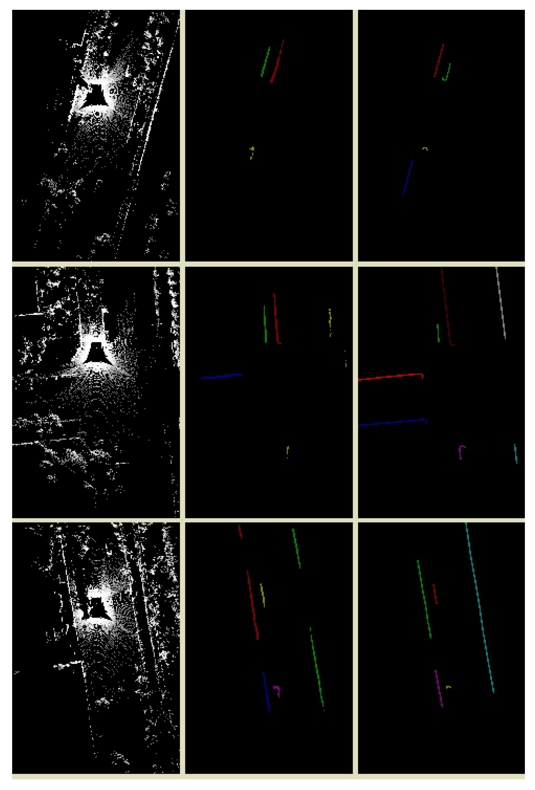
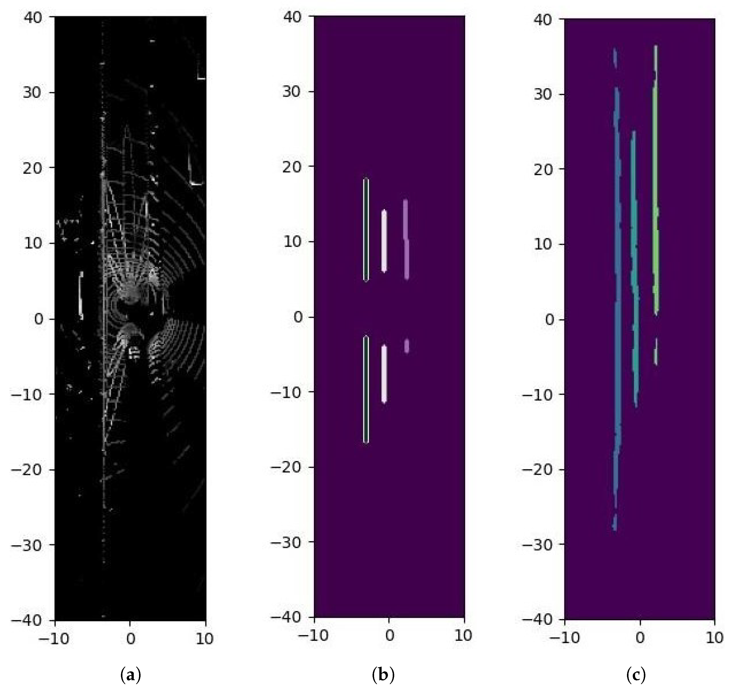
5.1. Methodology and Criteria for Data Presentation Selection

In the coordinate system of the ego vehicle, the direction of the road edge is generally considered the boundary of the vehicle’s lateral (y-axis) movement range. From the perspective of motion control, lateral constraints on the movement planning of autonomous logistic vehicles are primarily imposed, encompassing aspects such as lane selection and the obstacle avoidance strategy choices of the autonomous delivery vehicle. On the other hand, given the current situation in which autonomous logistic vehicles predominantly operate in urban-area bicycle lanes and exhibit a lower average traveling speed compared to passenger cars, the precision of predictions in the y-direction is relatively more critical than in the x-direction. Therefore, this study defines the area of interest for evaluating the proposed perception algorithms as the range shown in Figure 5. A resolution of 2 m in the near field and 3 m in the further field on the lateral side (y-direction) is utilized to ensure that the evaluation area sufficiently covers lane planning and prevents collisions with road edges. A resolution of 20 m in the longitudinal direction (x-axis) is adopted in order to meet the requirements for maintaining a safe following distance. Additionally, the evaluation metrics introduced in Section 4.4 are employed to calculate the quantified average perception performance within each segmented area.

The overall comparative experiments are conducted between modules “modified tri-plane BEV-encoder” and “M²BEV’s image-to-BEV feature projection” (Section 4.3), and both utilize the network architecture depicted in Figure 1. Specifically, in the experiments conducted for module “M²BEV’s image-to-BEV feature projection”, only the tri-plane module presented in Figure 1 was substituted with the module itself (with the same backbone, ResNet-34), with all the remaining components of the network unchanged. Concurrently, the experiment denoted as “fisheye rectification” refers to the network’s image preprocess of undistorting fisheye camera images based on calibration results and the rectification model described in Section 3.2. The result is shown in Table 1.

The comparative analysis of the effectiveness of different parts of the ROI region for the fisheye camera distortion correction method and the tri-plane BEV-encoder is presented in

Table 2. Recall result using proposed evaluation metrics in different parts of the ROI.

y_Range (m)	x_Range (m)	With Tri-Plane Encoder & without Fisheye Rectification	With Tri-Plane Encoder & with Fisheye Rectification	Without Tri-Plane Encoder & without Fisheye Rectification	Without Tri-Plane Encoder & with Fisheye Rectification
2~5	−40~−20	78.7%	80.6%	77.8%	77.8%
	−20~0	83.3%	79.7%	82.3%	82.6%
	0~20	71.2%	77.2%	72.5%	72.6%
	20~40	75.6%	69.7%	76.4%	76.2%
0~2	−40~−20	52.7%	48.2%	65.7%	61.2%
	−20~0	81.3%	78.5%	77.5%	75.3%
	0~20	58.6%	78.1%	49.9%	51.6%
	20~40	45.2%	75.0%	38.7%	41.7%
−2~0	−40~−20	58.9%	53.8%	63.8%	63.5%
	−20~0	93.4%	93.2%	87.4%	86.1%
	0~20	96.3%	96.1%	90.2%	89.6%
	20~40	71.8%	50.2%	70.9%	70.6%
−5~−2	−40~−20	80.8%	64.3%	81.3%	80.3%
	−20~0	57.7%	53.8%	52.0%	52.2%
	0~20	48.4%	56.2%	44.8%	45.3%
	20~40	59.3%	59.2%	60.9%	60.7%

and

Table 3. Precision result using proposed evaluation metrics in different parts of the ROI.

y_Range (m)	x_Range (m)	With Tri-Plane Encoder & without Fisheye Rectification	With Tri-Plane Encoder & with Fisheye Rectification	Without Tri-Plane Encoder & without Fisheye Rectification	Without Tri-Plane Encoder & with Fisheye Rectification
2~5	−40~−20	34.7%	43.0%	36.6%	37.4%
	−20~0	88.8%	91.4%	89.8%	89.9%
	0~20	88.9%	93.4%	89.6%	89.3%
	20~40	69.0%	75.5%	68.1%	68.1%
0~2	−40~−20	21.9%	44.2%	21.4%	21.2%
	−20~0	45.2%	65.6%	35.8%	37.3%
	0~20	64.7%	76.7%	42.4%	45.1%
	20~40	32.2%	54.5%	26.3%	26.9%
−2~0	−40~−20	39.8%	45.0%	36.3%	37.7%
	−20~0	64.5%	67.3%	57.6%	57.2%
	0~20	81.4%	81.6%	76.3%	75.7%
	20~40	43.9%	42.8%	44.0%	45.0%
−5~−2	−40~−20	82.6%	83.3%	82.3%	84.2%
	−20~0	82.6%	88.0%	81.0%	80.8%
	0~20	74.7%	88.5%	73.1%	73.3%
	20~40	65.6%	68.4%	62.6%	62.9%

.

Within a $\pm 40$-m range to the front and rear and a $\pm 5$-m range to the left and right in the vehicle’s coordinate system, both of the two proposed modules contribute to an improvement in detection accuracy for the curb detection network. The network’s inference results are visualized in Figure 6 and Figure 7.

5.2. Comparative Experimental Analysis of Algorithm Modules

From the results presented in Table 1, the following observations can be made:

• The modified tri-plane BEV-encoder module, compared to the M²BEV’s image-to-BEV feature projection module, demonstrated superior average precision and recall rates in the urban-area road experiments conducted for autonomous delivery vehicles in this article under conditions both with and without the fisheye rectification preprocessing step for fisheye camera images;
• The presence of a fisheye camera distortion correction preprocessing step showed relatively minor performance differentiation when neither of the above-mentioned spatial transformation modules were utilized. However, when employing the M²BEV’s image-to-BEV feature projection module, considering both the average accuracy and recall, the fisheye camera distortion correction preprocessing did not result in a notable improvement in performance. In contrast, with the implementation of the tri-plane encoder module, this preprocessing step led to a certain degree of performance enhancement.

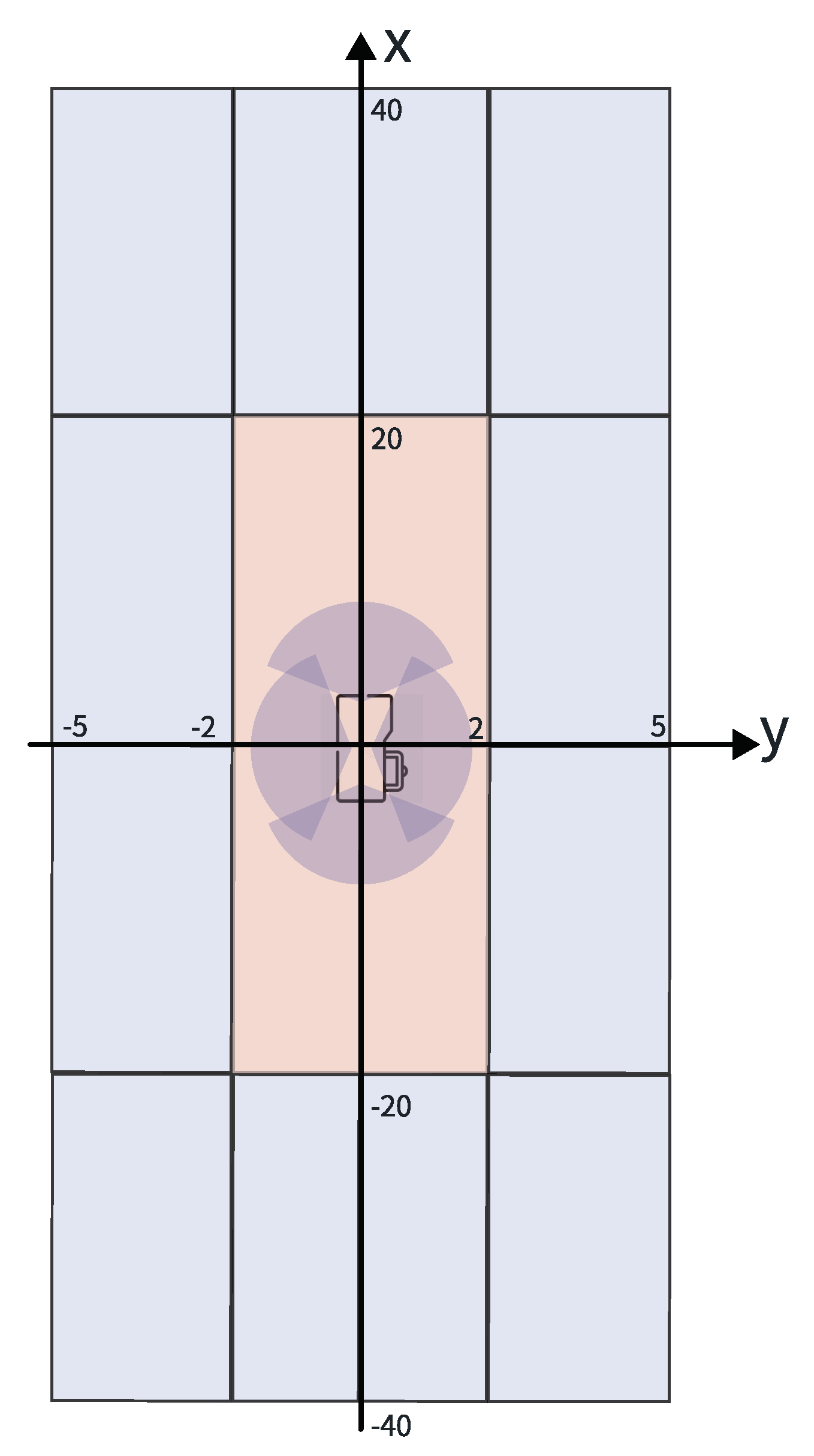
5.3. Performance Analysis of ROI Partitioning in Algorithms

This section conducts a quantitative analysis and discussion on the performance of the multi-modal curb detection network across different parts of the ROI for autonomous delivery vehicles. The evaluation aims to assess the network’s effectiveness in its applied scenario and whether its ability meets the task’s requirements.

According to the results presented in Table 2 and Table 3, the multi-modal network incorporating the tri-plane encoder and fisheye rectification module exhibits higher detection precision in areas close to the ego-vehicle (i.e., within $\pm 2$ m in the x-direction and $\pm 20$ m in the y-direction) than that in those more distant regions (i.e., $\pm 2$~$\pm 5$ m in the x-direction and $\pm 20$~$\pm 40$ m in the y-direction). In those further parts of ROI, although a certain degree of performance degradation is observed, detection precision remains above 50% on average. This performance reduction is consistent with the inherent properties of LiDAR point clouds, which are denser near the sensor and sparser at greater distances, and the challenges associated with detecting distant objects using visual detection algorithms.

Additionally, it is notable that, due to the test set’s characteristics, the average distribution of the curb in the ego-vehicle coordinate system does not guarantee strict symmetry. Furthermore, more sensors are mounted in the front side of the vehicle in order to obtain a robust perception result in the driving direction. Consequently, the evaluation metrics within the ROI do not exhibit spatial symmetry.

In summary, for applications involving autonomous delivery vehicles operating at relatively low speeds, the proposed multi-modal curb detection network demonstrates significant utility.

6. Conclusions

6.1. The Effectiveness of the Modified Tri-Plane Encoder

Based on the observations in Section 5.2, we can draw the following conclusions:

• The tri-plane BEV-encoder module, adapted and introduced from the domain of 3D image reconstruction, has shown potential for application in tasks such as curb detection. This is evidenced by its comparative analysis with an existing similar method, despite the well-acknowledged inherent randomness associated with deep learning-based approaches.
• The rectification of fisheye camera images contributes to an improvement in the performance of the aforementioned spatial transformation module.

6.2. The Effectiveness of the Proposed Multi-Modal Edge Detection Network

Based on the analysis presented in Section 5.3, it can be concluded that for applications involving autonomous delivery vehicles operating at relatively low speeds, the proposed multi-modal curb detection network exhibits a certain degree of utility.

6.3. Highlight of Contributions

The contributions of this paper are summarized as follows:

• The spatial transformation of features, particularly the conversion of image features to Bird’s Eye View (BEV) space, remains a focal issue in the field of autonomous driving detection. We observed that the tri-plane encoder within the EG3D network from the domain of 3D image reconstruction achieves a balance between parameter quantity and the volume of spatial representation information. Consequently, this feature space transformation module was fine-tuned and integrated into a multi-modal network.
• This paper introduces a multi-modal curb detection network that supports LiDAR, pinhole telephoto cameras, and fisheye cameras. In addition to the camera branch featured in the above-mentioned module, the network’s LiDAR branch employs one of the industry’s most widely used models from the PointPillar series; meanwhile, the task head for curb detection takes a weighted sum of a semantic segmentation loss in BEV space, a longitudinal and lateral detection offset loss in the BEV plane, and a clustering loss for different curb instances.
• We utilized a logistics vehicle equipped with LiDAR, pinhole telephoto, and fisheye cameras to collect 24,350 frames of real-world data on urban roads for training and testing the proposed model. This data also served to validate the effectiveness of the tri-plane encoder module and assess the impact of fisheye camera image distortion removal preprocessing on the network relative to a baseline comparison.
• Based on the results analyzed, the introduced tri-plane encoder module exhibits considerable performance in curb detection tasks. Furthermore, the proposed multi-modal curb detection network meets the fundamental application requirements for this scenario.

6.4. Limitations and Future Directions of the Study

Within this paper, the following research limitations and inadequacies are acknowledged, which can be discussed in further research:

• A fisheye camera correction model of limited precision was employed, without comparison to more refined correction models or novel correction modules based on GAN networks, etc.
• The study did not subdivide specific curb scenarios and hard case for detection, which would have allowed for targeted optimization in scenarios where the detection algorithm under performs.
• The introduced tri-plane encoder module requires further investigation into these aspects:
  • Its placement relative to other components of the network, such as being positioned before the FPN module or integrated within it;
  • The optimization of voxel resolution settings in relation to the ego-vehicle’s ROI size.

References

1. Siegemund, J.; Pfeiffer, D.; Franke, U.; Farstner, W. Curb reconstruction using Conditional Random Fields. In Proceedings of the IEEE Intelligent Vehicles Symposium (IV), La Jolla, CA, USA, 21–24 June 2010; pp. 203–210. [Google Scholar]
2. Panev, S.; Vicente, F.; De la Torre, F.; Prinet, V. Road Curb Detection and Localization with Monocular Forward-View Vehicle Camera. IEEE Trans. Intell. Transp. Syst. 2018, 20, 3568–3584. [Google Scholar] [CrossRef]
3. Mi, X.; Yang, B.; Dong, Z.; Chen, C.; Gu, J. Automated 3D Road Boundary Extraction and Vectorization Using MLS Point Clouds. IEEE Trans. Intell. Transp. Syst. 2021, 23, 5287–5297. [Google Scholar] [CrossRef]
4. Rato, D.; Santos, V. LIDAR based detection of road boundaries using the density of accumulated point clouds and their gradients. Robot. Auton. Syst. 2021, 138, 103714. [Google Scholar] [CrossRef]
5. Deac, S.E.C.; Giosan, I.; Nedevschi, S. Curb detection in urban traffic scenarios using LiDARs point cloud and semantically segmented color images. In Proceedings of the IEEE Intelligent Transportation Systems Conference (ITSC), Auckland, New Zealand, 27–30 October 2019; pp. 3433–3440. [Google Scholar]
6. Ma, L.; Li, Y.; Li, J.; Marcato Junior, J.; Nunes Gonçalves, W.; Chapman, M. BoundaryNet: Extraction and Completion of Road Boundaries with Deep Learning Using Mobile Laser Scanning Point Clouds and Satellite Imagery. IEEE Trans. Intell. Transp. Syst. 2021, 23, 5638–5654. [Google Scholar] [CrossRef]
7. Schneider, D.; Schwalbe, E.; Maas, H.G. Validation of geometric models for fisheye lenses. ISPRS J. Photogramm. Remote Sens. 2009, 64, 259–266. [Google Scholar] [CrossRef]
8. Liao, K.; Lin, C.; Zhao, Y.; Gabbouj, M. DR-GAN: Automatic radial distortion rectification using conditional GAN in real-time. IEEE Trans. Circuits Syst. Video Technol. 2019, 30, 725–733. [Google Scholar] [CrossRef]
9. Liao, K.; Lin, C.; Zhao, Y.; Xu, M. Model-free distortion rectification framework bridged by distortion distribution map. IEEE Trans. Image Process. 2020, 29, 3707–3718. [Google Scholar] [CrossRef]
10. Philion, J.; Fidler, S. Lift, splat, shoot: Encoding images from arbitrary camera rigs by implicitly unprojecting to 3d. In Computer Vision–ECCV 2020, Proceedings of the 16th European Conference, Glasgow, UK, 23–28 August 2020; Proceedings, Part XIV 16; Springer International Publishing: Berlin/Heidelberg, Germany, 2020; pp. 194–210. [Google Scholar]
11. Chen, S.; Cheng, T.; Wang, X.; Meng, W.; Zhang, Q.; Liu, W. Efficient and robust 2d-to-bev representation learning via geometry-guided kernel transformer. arXiv 2022, arXiv:2206.04584. [Google Scholar]
12. Wang, Y.; Guizilini, V.C.; Zhang, T.; Wang, Y.; Zhao, H.; Solomon, J. Detr3d: 3d object detection from multi-view images via 3d-to-2d queries. In Conference on Robot Learning; PMLR: Baltimore, MD, USA, 2022; pp. 180–191. [Google Scholar]
13. Karras, T.; Aittala, M.; Hellsten, J.; Laine, S.; Lehtinen, J.; Aila, T. Training generative adversarial networks with limited data. In Proceedings of the Advances in Neural Information Processing Systems (NeurIPS), Virtual, 6–12 December 2020; Volume 33, pp. 12104–12114. [Google Scholar]
14. Oechsle, M.; Peng, S.; Geiger, A. UNISURF: Unifying neural implicit surfaces and radiance fields for multi-view reconstruction. In Proceedings of the IEEE International Conference on Computer Vision (ICCV), Montreal, BC, Canada, 11–17 October 2021. [Google Scholar]
15. Mildenhall, B.; Srinivasan, P.P.; Tancik, M.; Barron, J.T.; Ramamoorthi, R.; Ng, R. Nerf: Representing scenes as neural radiance fields for view synthesis. Commun. ACM 2021, 65, 99–106. [Google Scholar] [CrossRef]
16. Lombardi, S.; Simon, T.; Saragih, J.; Schwartz, G.; Lehrmann, A.; Sheikh, Y. Neural volumes: Learning dynamic renderable volumes from images. ACM Trans. Graph. 2019, 38, 1–14. [Google Scholar] [CrossRef]
17. Reiser, C.; Peng, S.; Liao, Y.; Geiger, A. KiloNeRF: Speeding up neural radiance fields with thousands of tiny MLPs. In Proceedings of the IEEE International Conference on Computer Vision (ICCV), Montreal, BC, Canada, 11–17 October 2021. [Google Scholar]
18. DeVries, T.; Bautista, M.A.; Srivastava, N.; Taylor, G.W.; Susskind, J.M. Unconstrained scene generation with locally conditioned radiance fields. arXiv 2021, arXiv:2104.00670. [Google Scholar]
19. Chan, E.R.; Lin, C.Z.; Chan, M.A.; Nagano, K.; Pan, B.; De Mello, S.; Gallo, O.; Guibas, L.J.; Tremblay, J.; Khamis, S.; et al. Efficient geometry-aware 3D generative adversarial networks. In Proceedings of the IEEE/CVF Conference on Computer Vision and Pattern Recognition, New Orleans, LA, USA, 18–24 June 2022; pp. 16123–16133. [Google Scholar]
20. Zhu, X.; Su, W.; Lu, L.; Li, B.; Wang, X.; Dai, J. Deformable detr: Deformable transformers for end-to-end object detection. arXiv 2020, arXiv:2010.04159. [Google Scholar]
21. Kannala, J.; Brandt, S.S. A generic camera model and calibration method for conventional, wide-angle, and fish-eye lenses. IEEE Trans. Pattern Anal. Mach. Intell. 2006, 28, 1335–1340. [Google Scholar] [CrossRef]
22. OpenCV Documentation. Available online: https://docs.opencv.org/3.4/db/d58/group__calib3d__fisheye.html (accessed on 4 March 2024).
23. OpenCV Documentation. Available online: https://docs.opencv.org/3.4/da/d54/group__imgproc__transform.html#gab75ef31ce5cdfb5c44b6da5f3b908ea4 (accessed on 4 March 2024).
24. Chen, K.; Wang, J.; Pang, J.; Cao, Y.; Xiong, Y.; Li, X.; Sun, S.; Feng, W.; Liu, Z.; Xu, J.; et al. MMDetection: Open MMLab Detection Toolbox and Benchmark. arXiv 2019, arXiv:1906.07155. [Google Scholar]
25. Lang, A.H.; Vora, S.; Caesar, H.; Zhou, L.; Yang, J.; Beijbom, O. Pointpillars: Fast encoders for object detection from point clouds. In Proceedings of the IEEE/CVF Conference on Computer Vision and Pattern Recognition, Long Beach, CA, USA, 15–20 June 2019; pp. 12697–12705. [Google Scholar]
26. Yan, Y.; Mao, Y.; Li, B. Second: Sparsely embedded convolutional detection. Sensors 2018, 18, 3337. [Google Scholar] [CrossRef] [PubMed]
27. Xie, E.; Yu, Z.; Zhou, D.; Philion, J.; Anandkumar, A.; Fidler, S.; Luo, P.; Alvarez, J.M. M2BEV: Multi-Camera Joint 3D Detection and Segmentation with Unified Birds-Eye View Representation. arXiv 2022, arXiv:2204.05088. [Google Scholar]
28. Huang, B.; Li, Y.; Xie, E.; Liang, F.; Wang, L.; Shen, M.; Liu, F.; Wang, T.; Luo, P.; Shao, J. Fast-BEV: Towards Real-time On-vehicle Bird’s-Eye View Perception. arXiv 2023, arXiv:2301.07870. [Google Scholar]
Figure 1. The architecture of the proposed modified tri-plane BEV-encoder taking a single camera input as an example. (The blue sphere represents the feature map value of the position ( x , y , y ) in the 3D feature-map grid coordinates).
Vehicles 06 00024 g001
Figure 2. The general, radially symmetric projection model proposed by Kannala and Brandt. The image of the point P is p, whereas it would be p in the case of a pinhole camera.
Vehicles 06 00024 g002
Figure 3. The framework of the proposed curb detection network.
Vehicles 06 00024 g003
Figure 4. Fisheye camera undistortion test visualization. (a) Raw fisheye camera image. (b) Rectified fisheye camera image using Kannala–Brandt model.
Vehicles 06 00024 g004
Figure 5. Schematic diagram of the evaluation region of interest with dimensions in meters.
Vehicles 06 00024 g005
Figure 6. Curb detection network result visualization, where different colors represent different instances. (the unit of the distance range is meters). (a) LiDAR points in BEV perspective. (b) Ground truth curb instance. (c) Predicted curb instance.
Vehicles 06 00024 g006
Figure 7. Schematic illustration of curb detection results. From right to left, the first to third columns represent the LiDAR points BEV diagram, ground truth annotations of curb instances on the BEV plane, and visualization of the network’s detection results, respectively. (Different colors represent different curb instances).
Vehicles 06 00024 g007