
Cooperative Vehicle Localization in Multi-Sensor Multi-Vehicle Systems Based on an Interval Split Covariance Intersection Filter with Fault Detection and Exclusion


Abstract
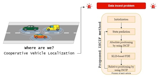
1. Introduction
- The ISCIF algorithm is proposed and implemented for vehicle localization in MSMVs in both absolute and relative positioning steps.
- The proposed ISCIF method can avoid the inverse of the interval matrix compared with the IEKF.
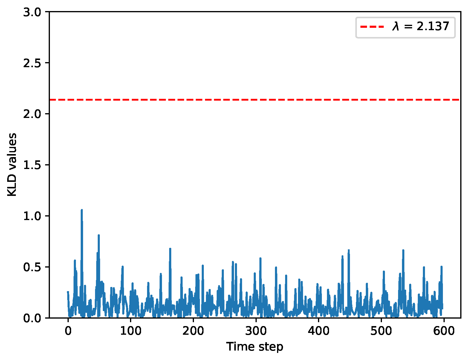
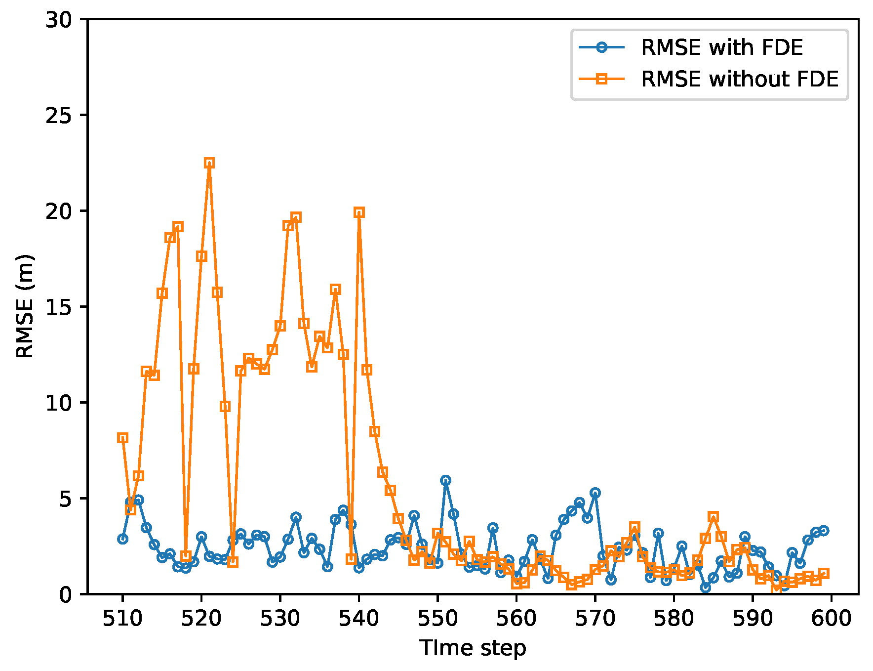
- A KLD-based FDE method is implemented to reduce the RMSE of the localization results when faults are present in the system.
- Based on the simulation results, our proposed method can achieve better accuracy than that of the SCIF. In addition, the implemented FDE method can achieve better accuracy when faults are present in the system.
2. Related Techniques and the Proposed ISCIF
2.1. Interval Analysis
2.2. Interval Constraint Propagation (ICP)
2.3. Interval Kalman Filter (IKF) and the Proposed Interval Split Covariance Intersection Filter
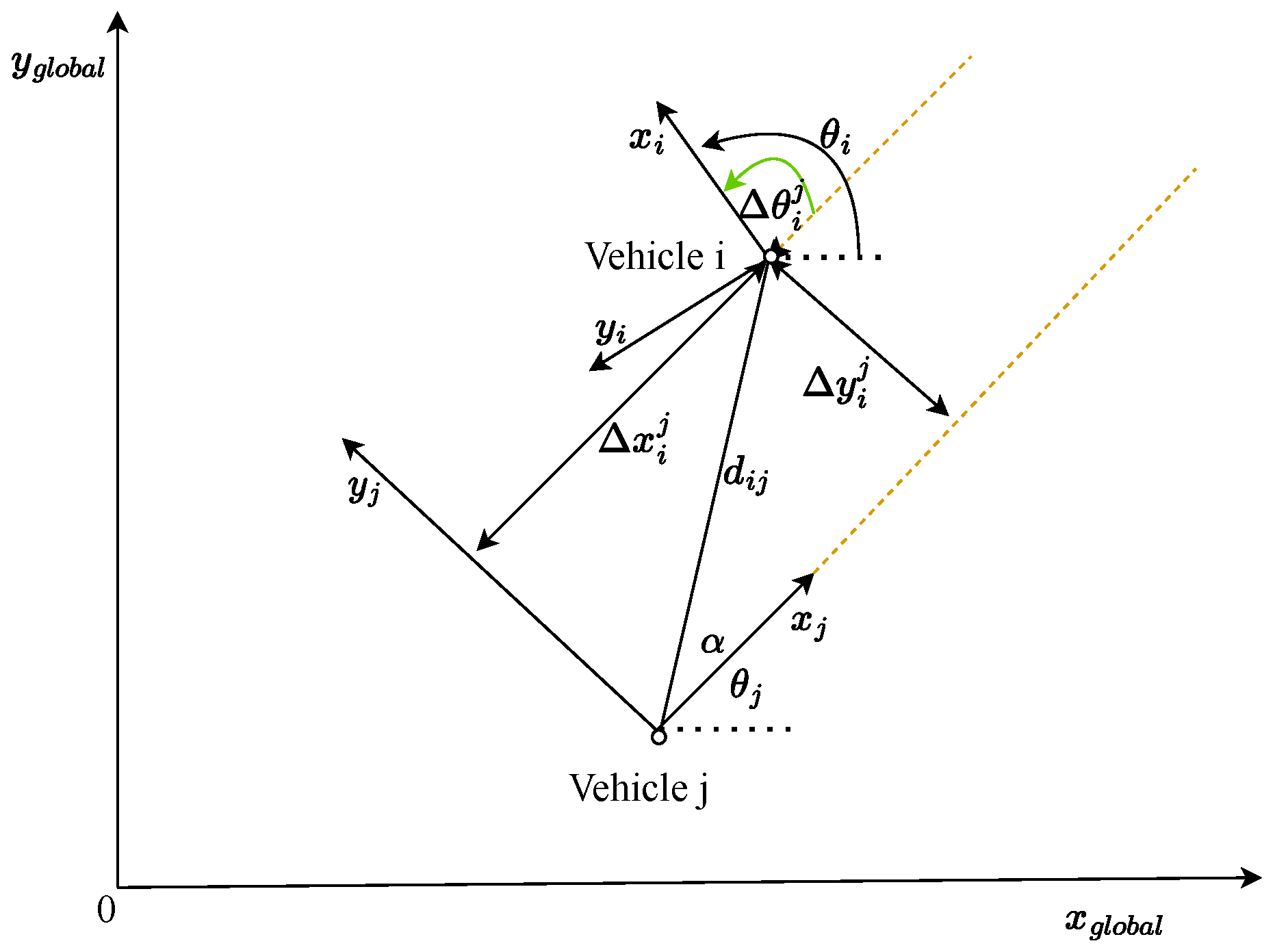
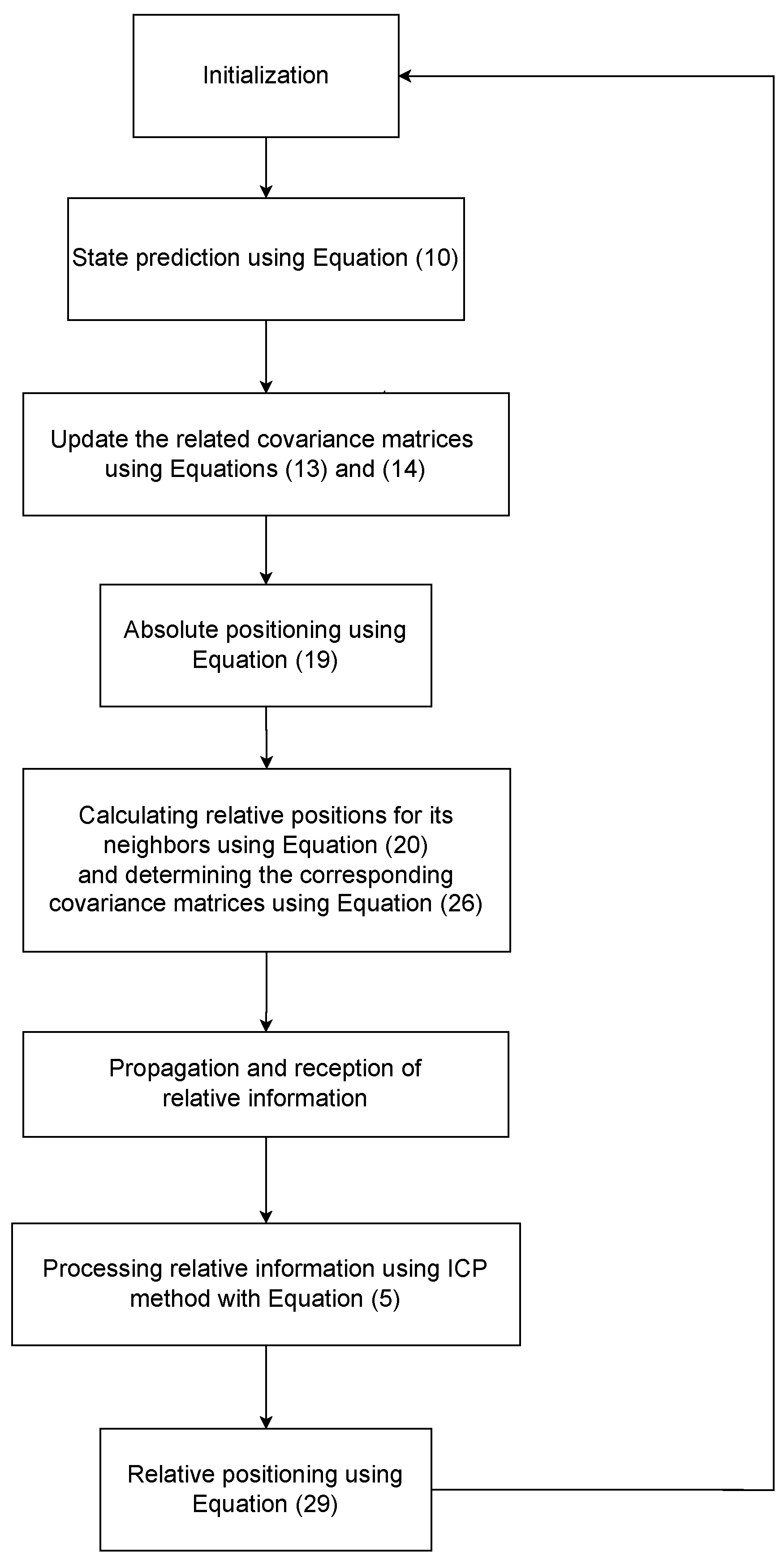
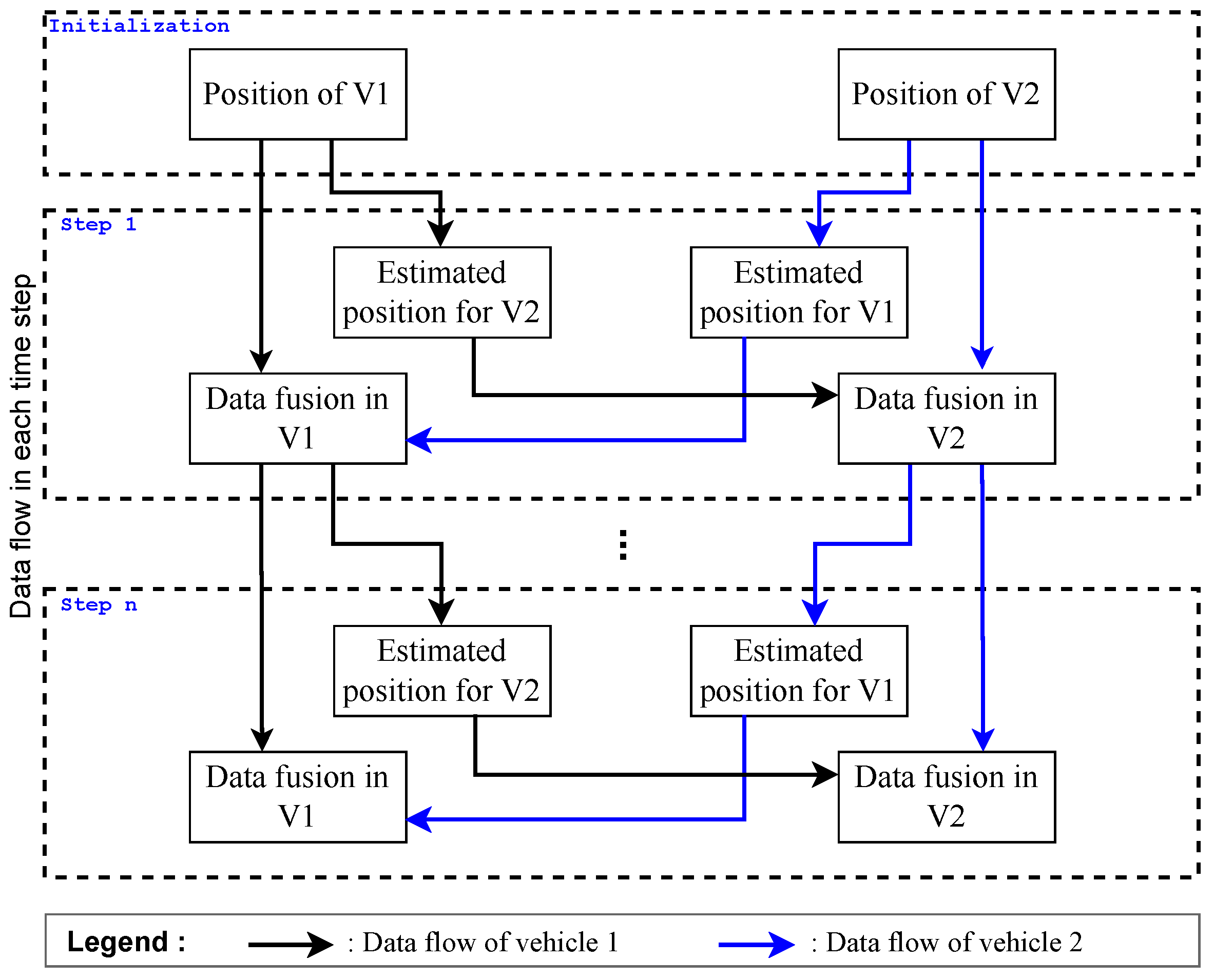
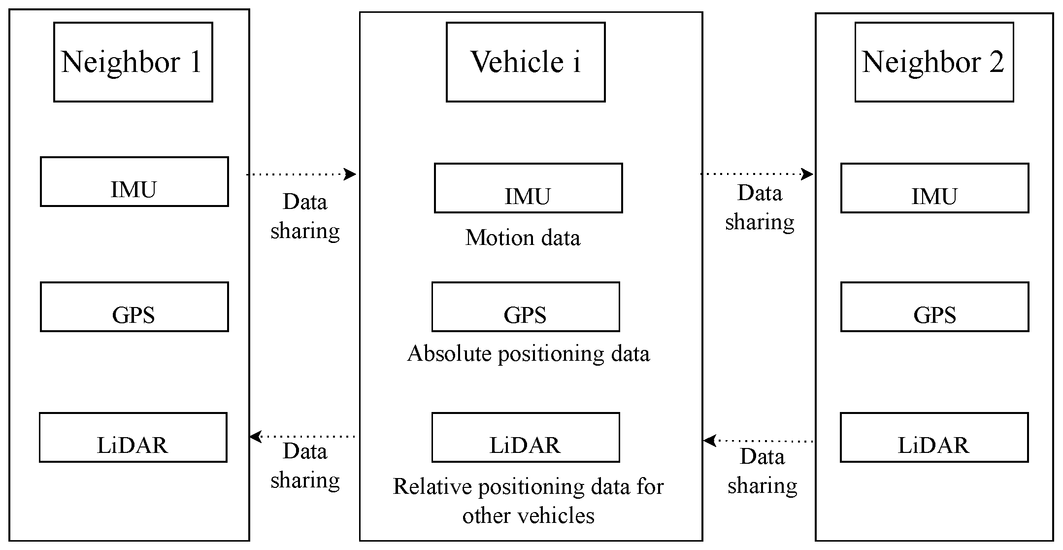
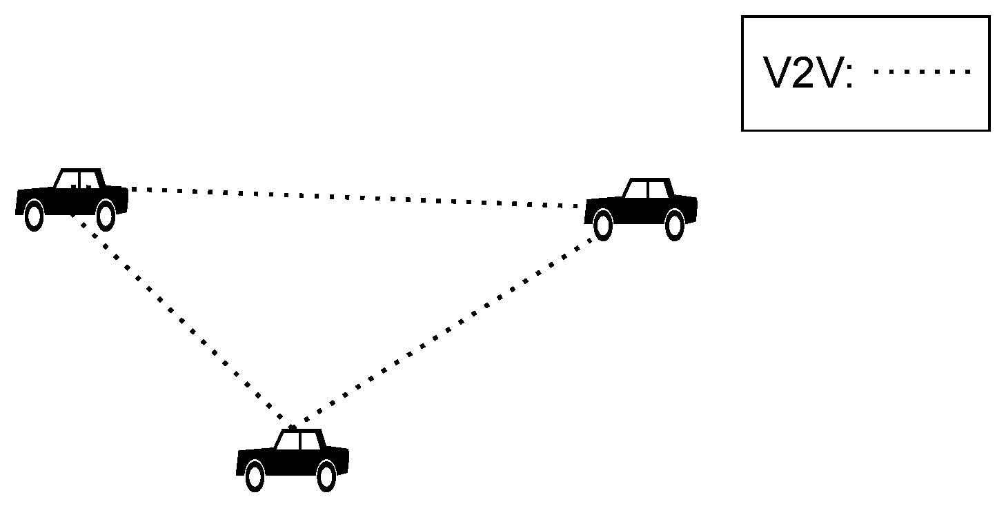
3. Cooperative Vehicle Localization with MSMVs by Using the ISCIF
3.1. System Model
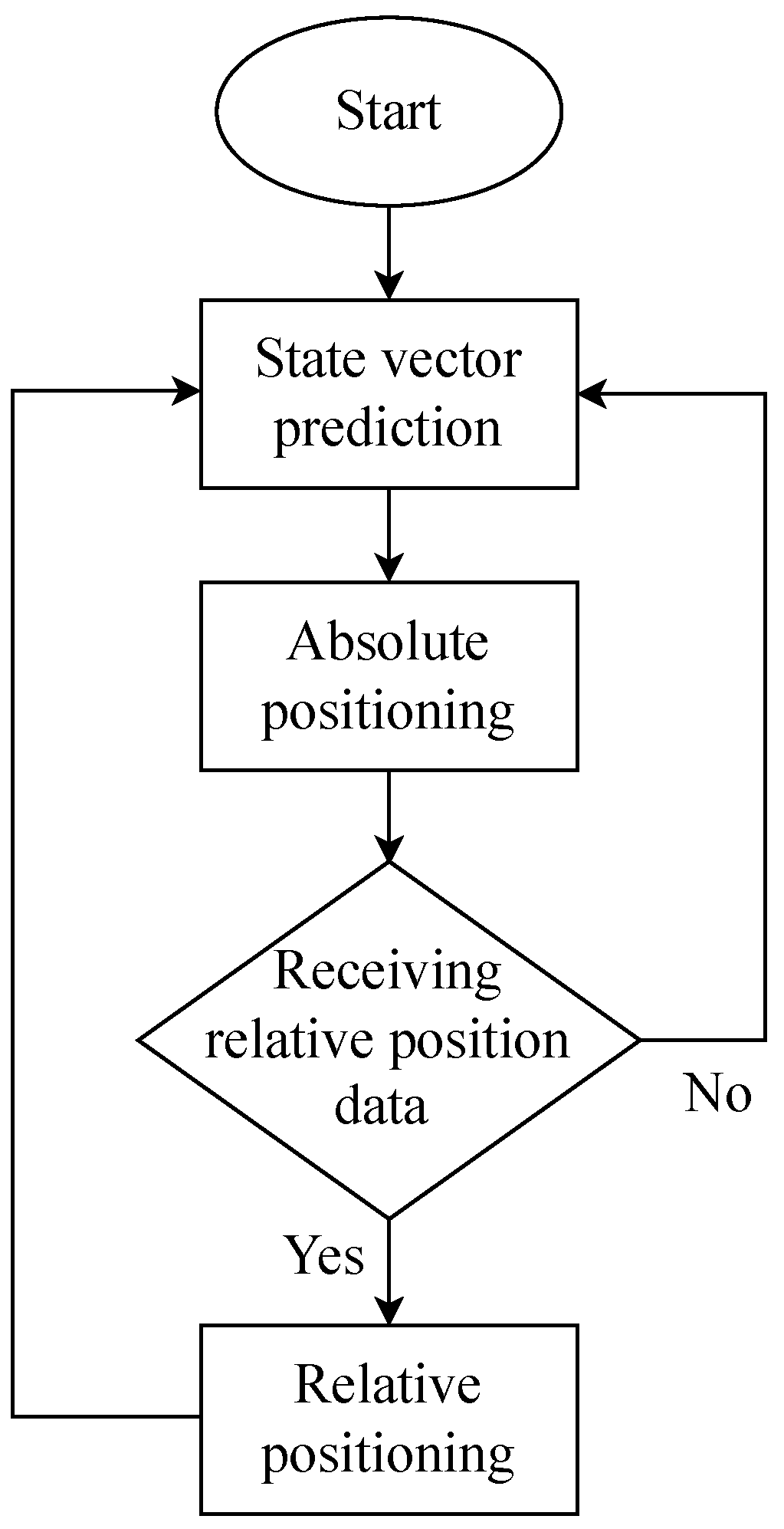
3.2. Prediction of the State Vector
3.3. Absolute Positioning
3.4. Relative Positioning
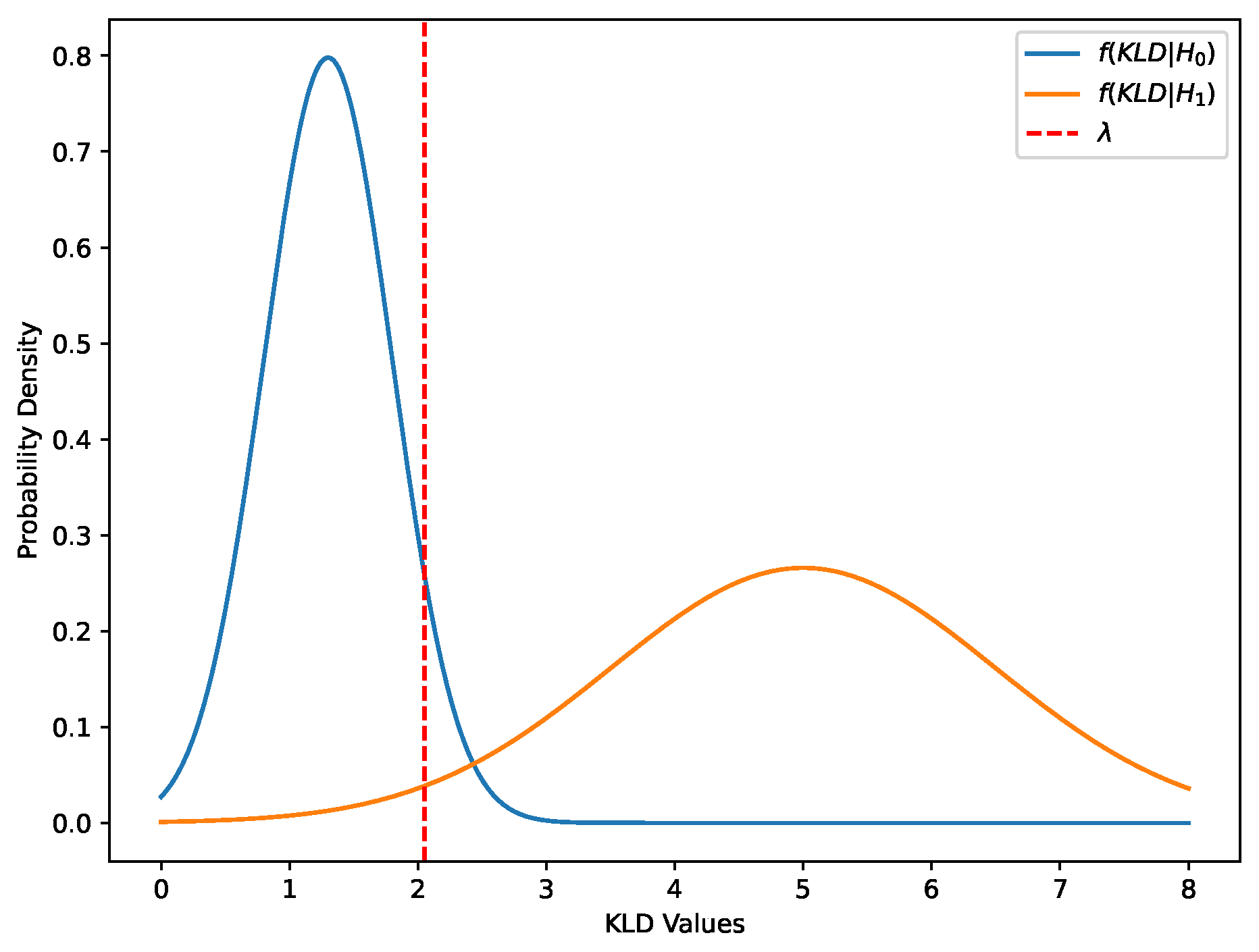
4. Fault Detection and Exclusion
5. Simulation Results
5.1. Simulation Scenarios and Parameters
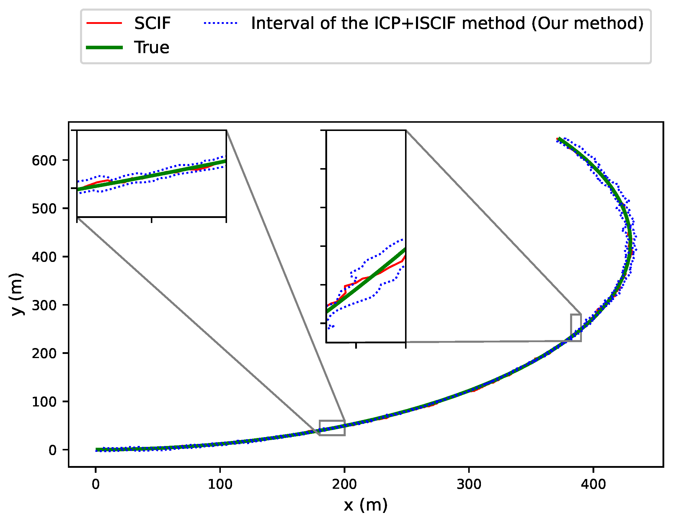
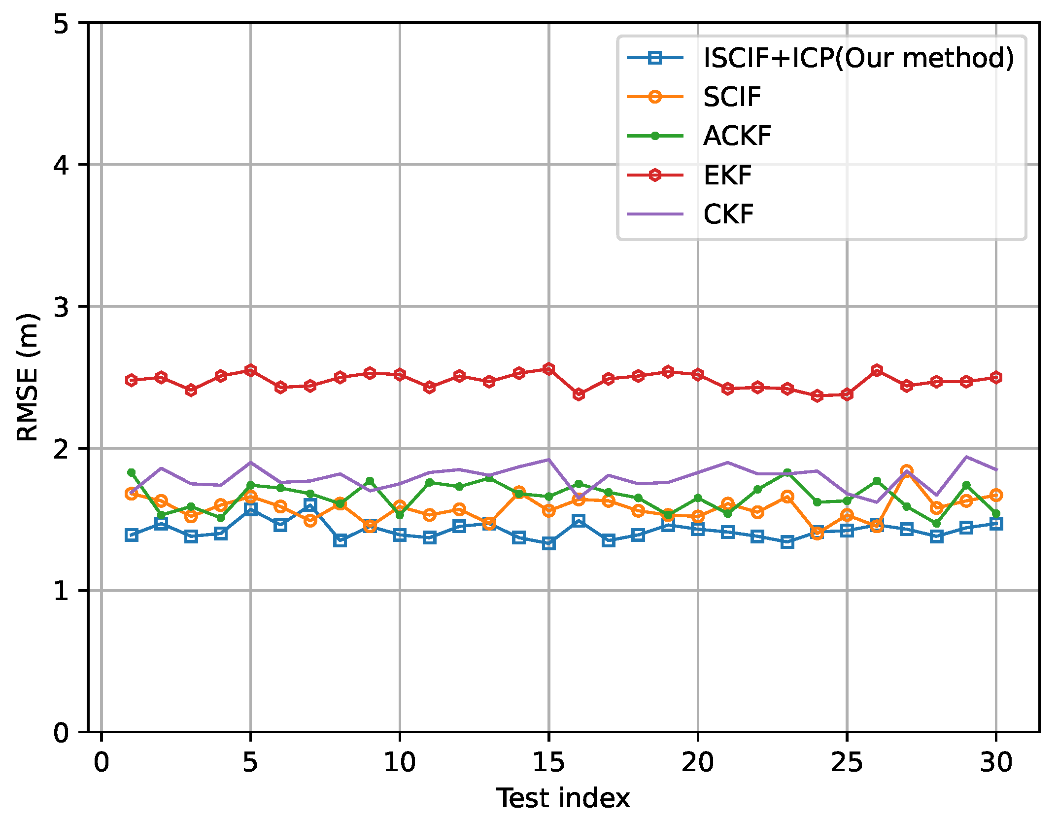
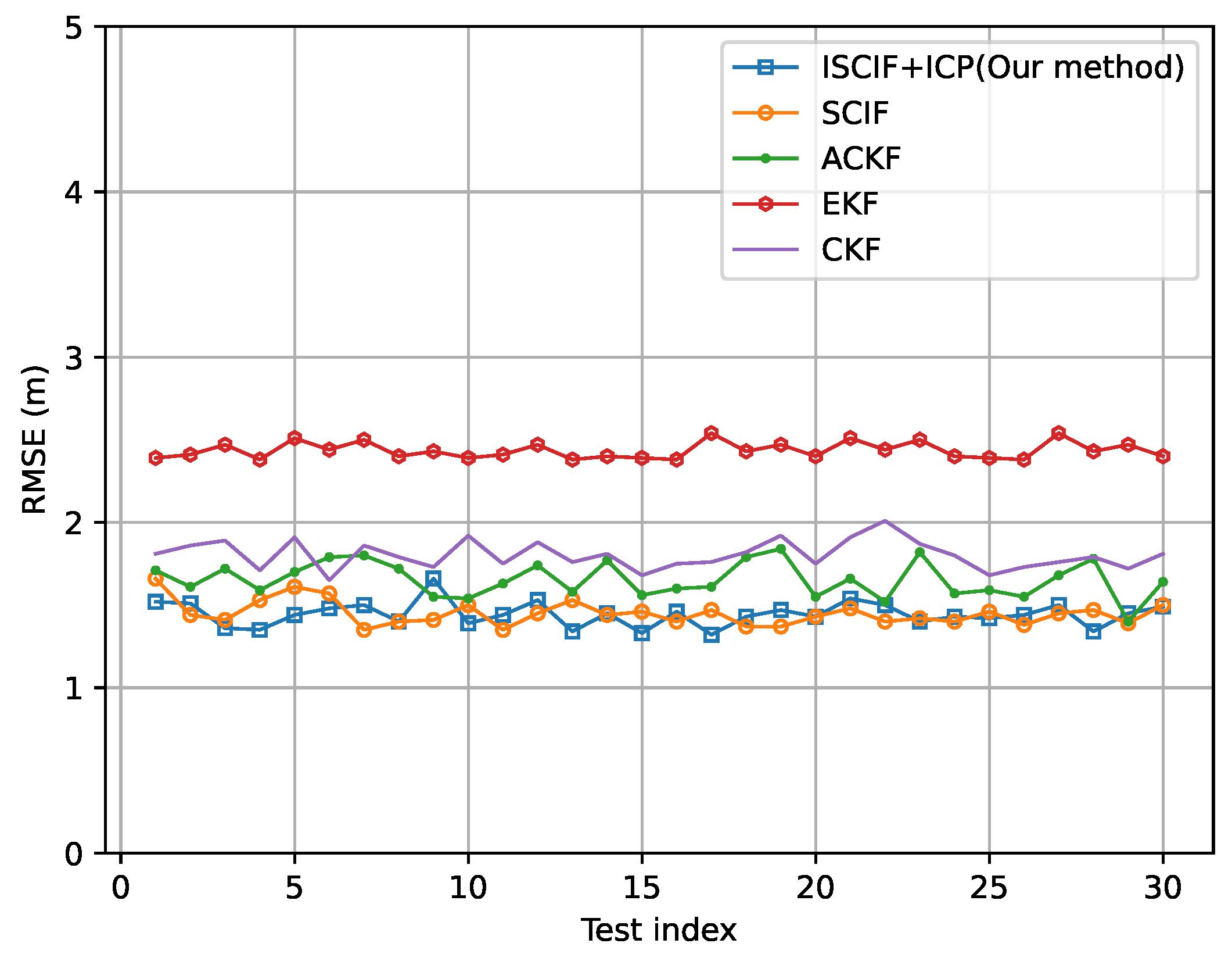
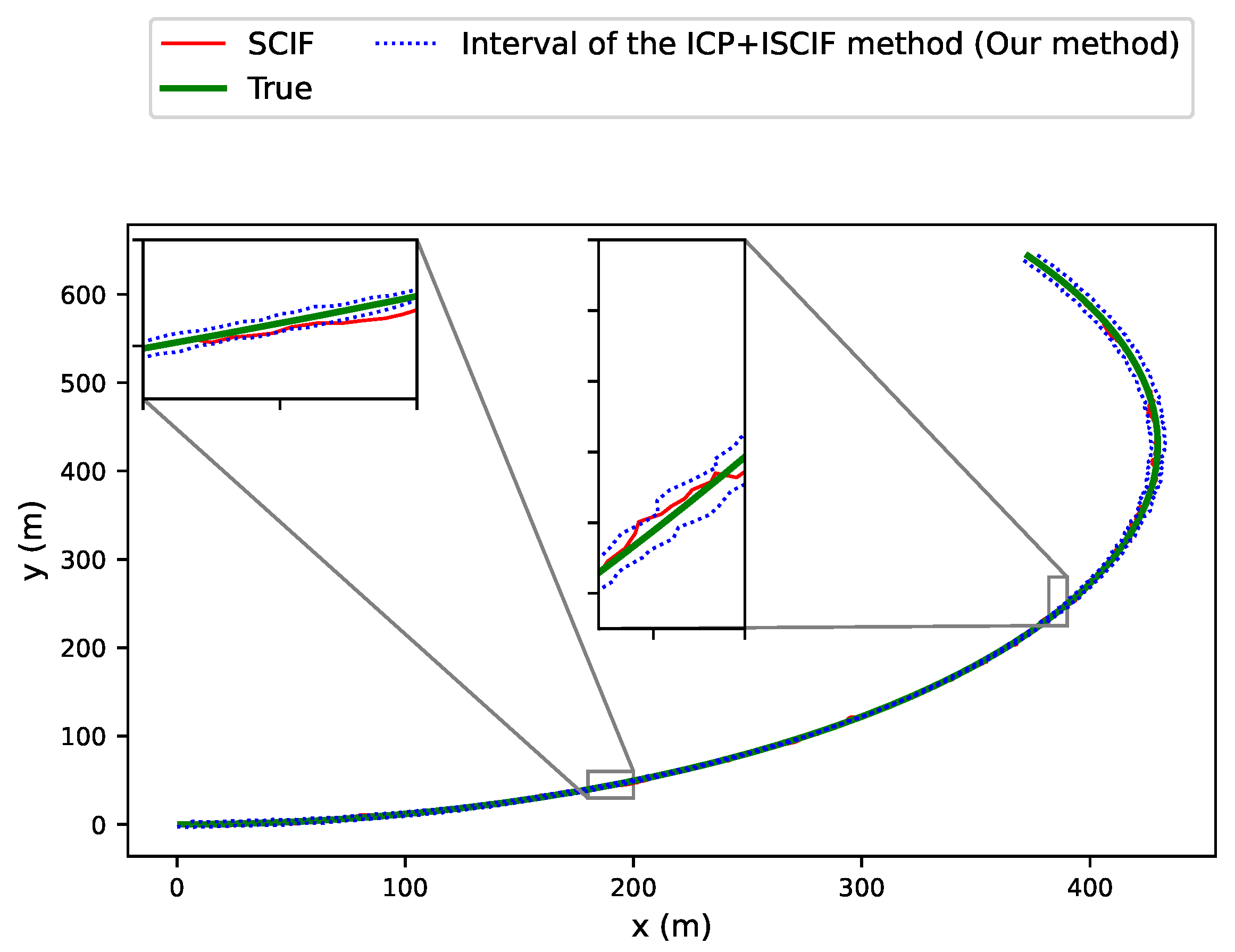
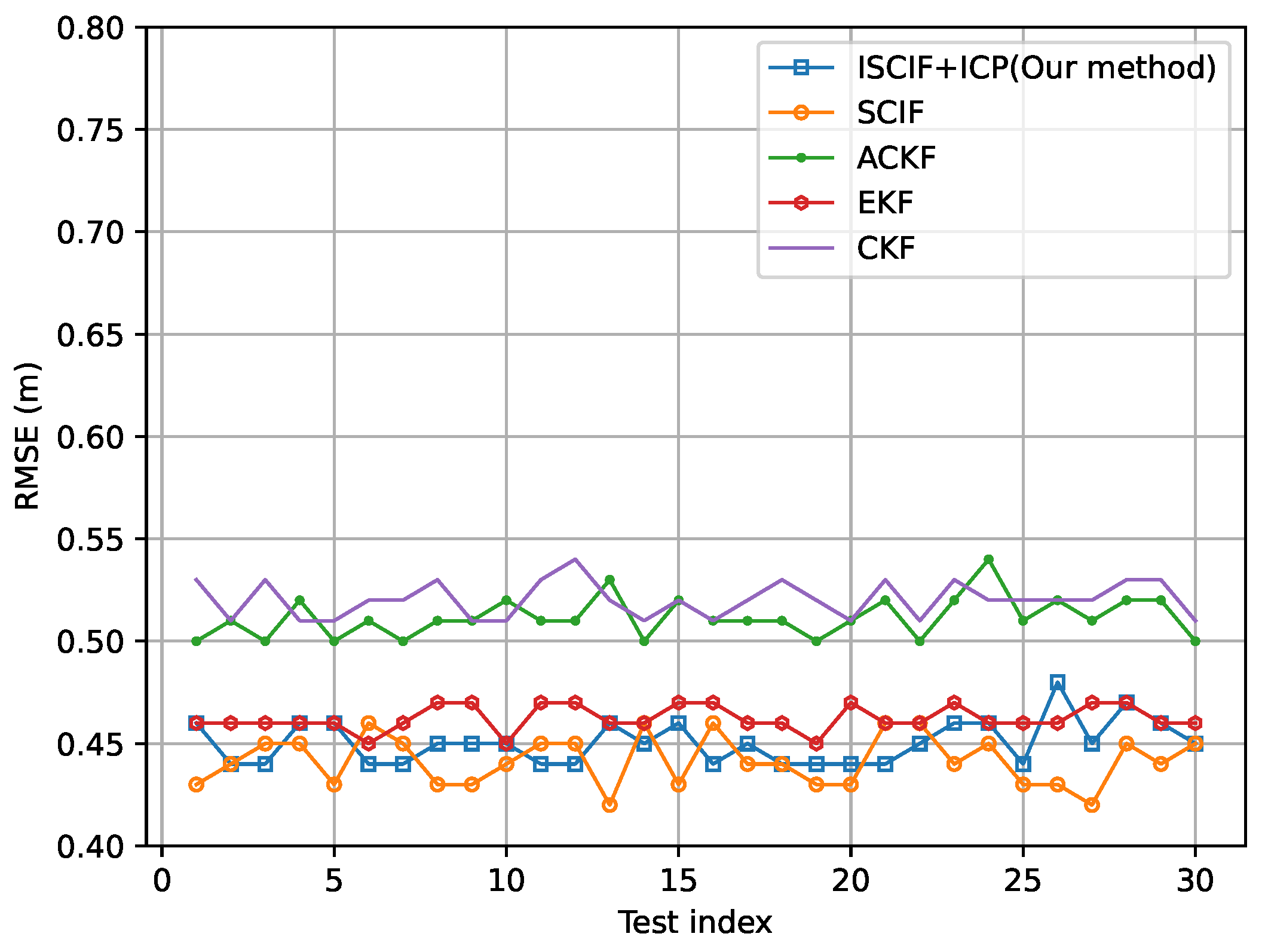
5.2. Results of Scenario 1: All Vehicles Have the Same Absolute Positioning Ability
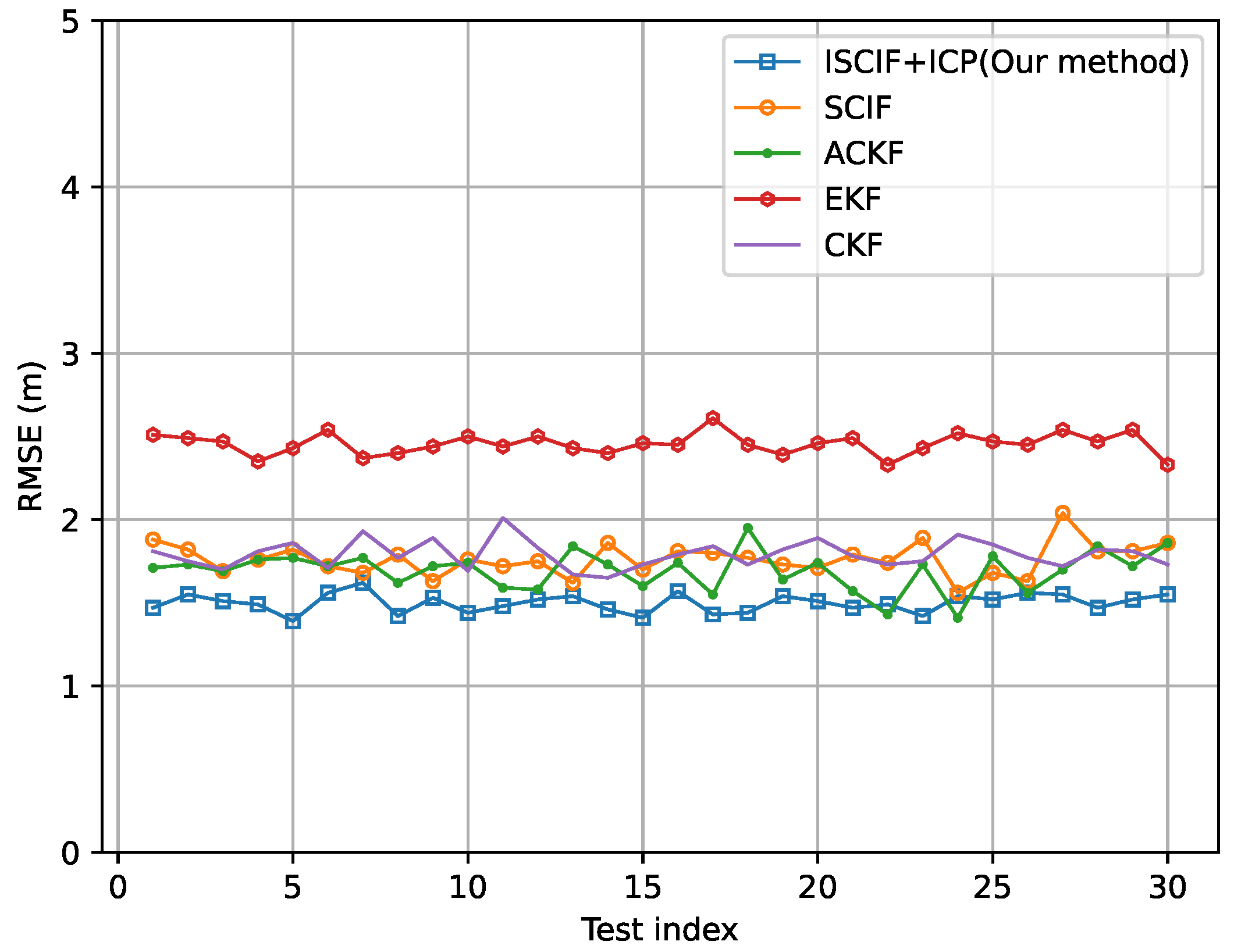
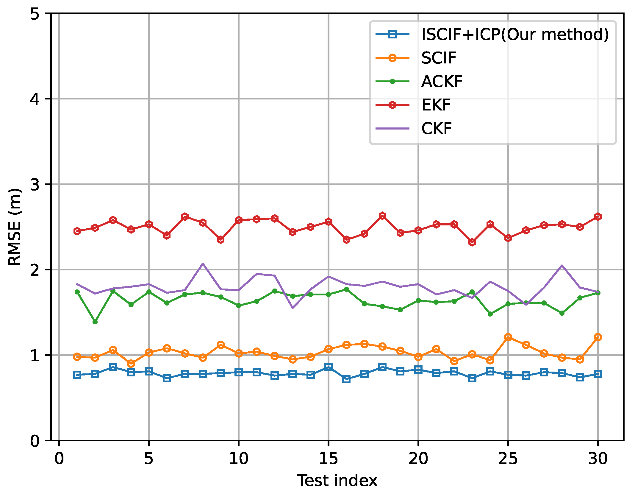
5.3. Results of Scenario 2: One Vehicle Has an Excellent Absolute Positioning Ability
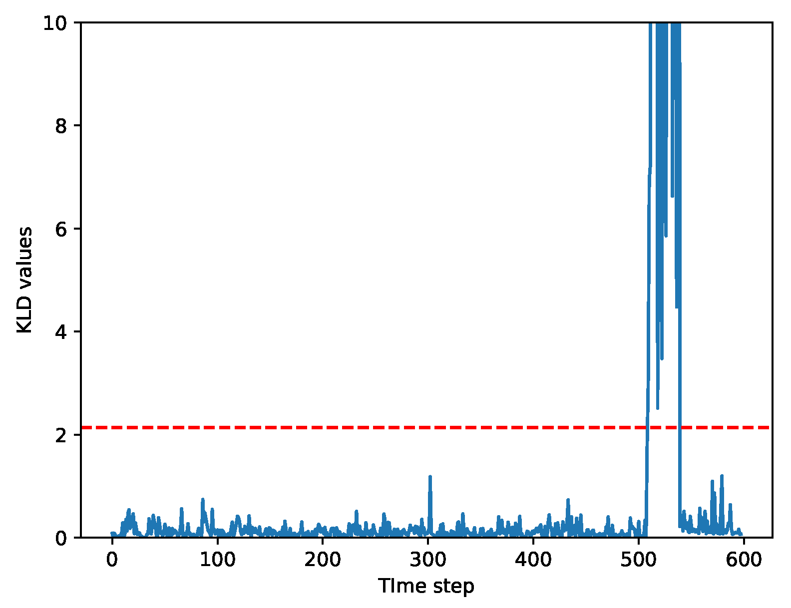
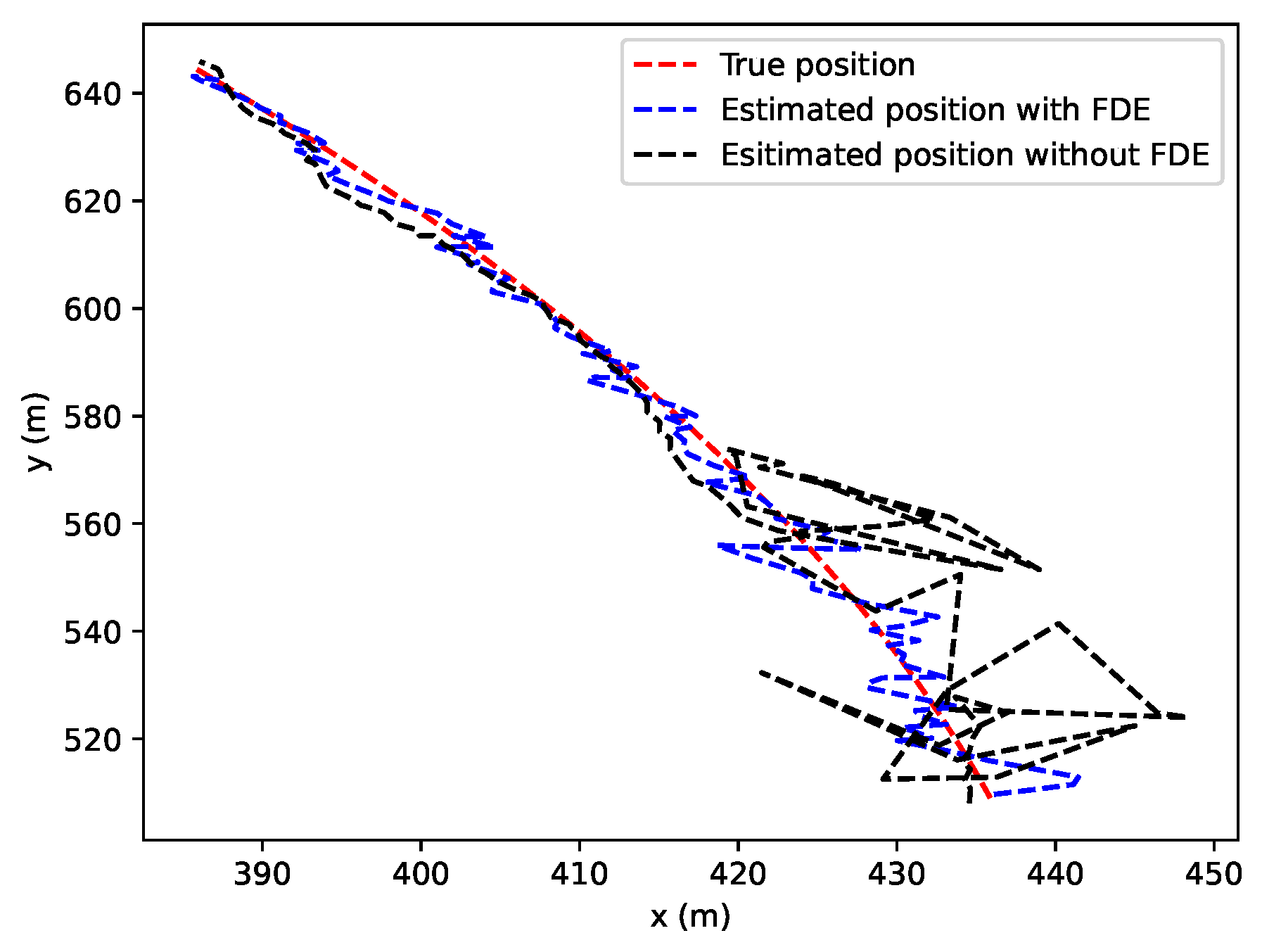
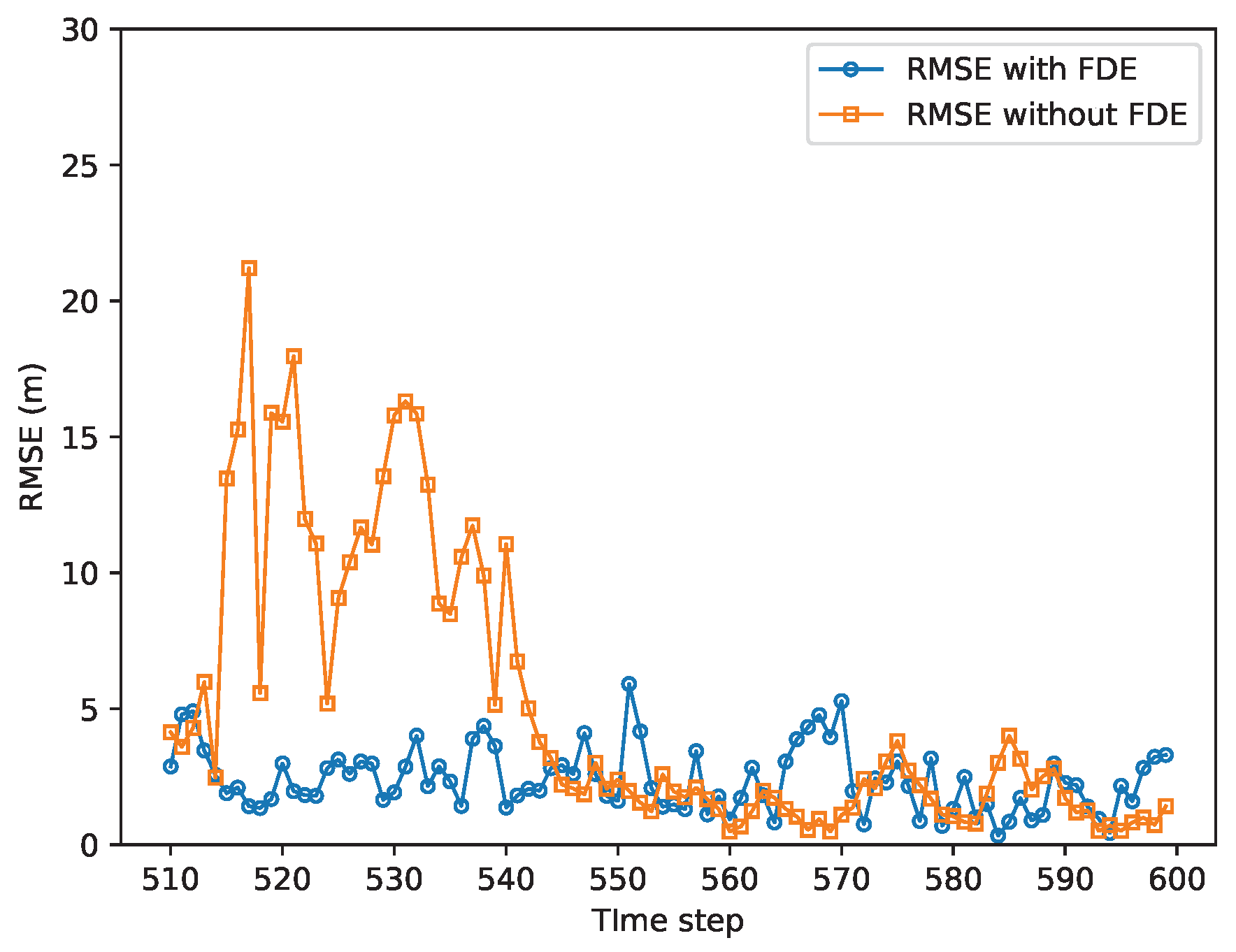
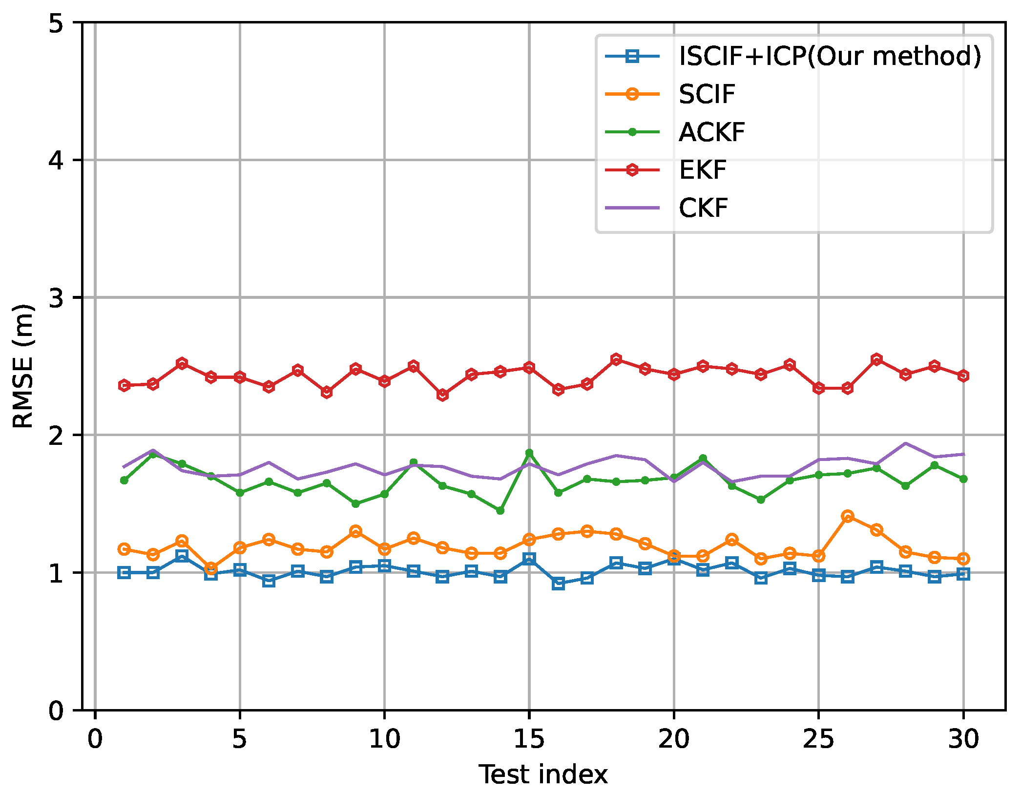
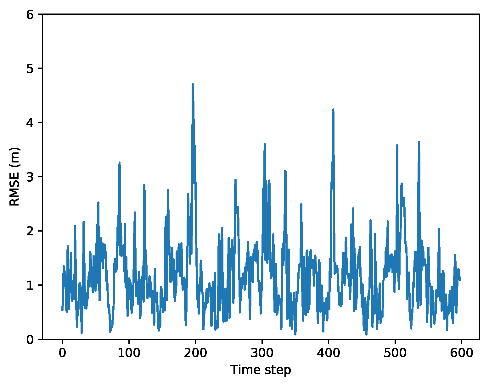
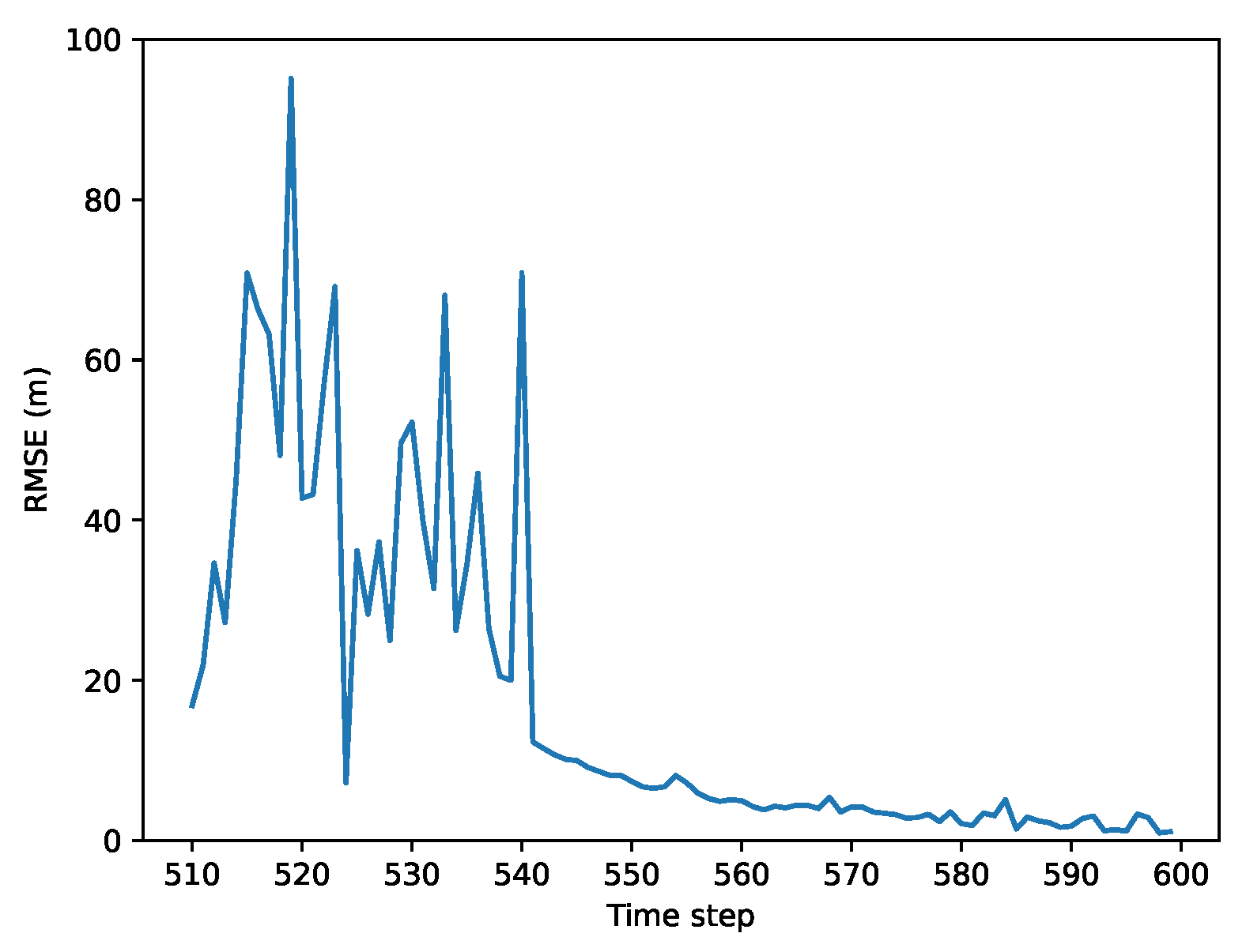
5.4. Results of Scenario 3: Cooperative Vehicle Localization with FDE
6. Conclusions and Future Work
Author Contributions
Funding
Data Availability Statement
Conflicts of Interest
References
- Alkendi, Y.; Seneviratne, L.; Zweiri, Y. State of the art in vision-based localization techniques for autonomous navigation systems. IEEE Access 2021, 9, 76847–76874. [Google Scholar] [CrossRef]
- Chen, G.; Lu, F.; Li, Z.; Liu, Y.; Dong, J.; Zhao, J.; Yu, J.; Knoll, A. Pole-curb fusion based robust and efficient autonomous vehicle localization system with branch-and-bound global optimization and local grid map method. IEEE Trans. Veh. Technol. 2021, 70, 11283–11294. [Google Scholar] [CrossRef]
- Cai, Y.; Lu, Z.; Wang, H.; Chen, L.; Li, Y. A lightweight feature map creation method for intelligent vehicle localization in urban road environments. IEEE Trans. Instrum. Meas. 2022, 71, 8503115. [Google Scholar] [CrossRef]
- Burghal, D.; Phadke, G.; Nair, A.; Wang, R.; Pan, T.; Algafis, A.; Molisch, A.F. Supervised learning approach for relative vehicle localization using V2V MIMO links. In Proceedings of the ICC 2022-IEEE International Conference on Communications, Seoul, Republic of Korea, 16–20 May 2022; pp. 4528–4534. [Google Scholar] [CrossRef]
- Rivoirard, L.; Wahl, M.; Sondi, P.; Gruyer, D.; Berbineau, M. A cooperative vehicle ego-localization application using v2v communications with cbl clustering. In Proceedings of the 2018 IEEE Intelligent Vehicles Symposium (IV), Suzhou, China, 26–30 June 2018; pp. 722–727. [Google Scholar] [CrossRef]
- Randriamasy, M.; Cabani, A.; Chafouk, H.; Fremont, G. Reliable vehicle location in electronic toll collection service with cooperative intelligent transportation systems. In Proceedings of the 2017 IEEE 28th Annual International Symposium on Personal, Indoor, and Mobile Radio Communications (PIMRC), Montreal, QC, Canada, 8–13 October 2017; pp. 1–7. [Google Scholar] [CrossRef]
- Randriamasy, M.; Cabani, A.; Chafouk, H.; Fremont, G. Geolocation process to perform the electronic toll collection using the ITS-G5 technology. IEEE Trans. Veh. Technol. 2019, 68, 8570–8582. [Google Scholar] [CrossRef]
- Fascista, A.; Ciccarese, G.; Coluccia, A.; Ricci, G. A localization algorithm based on V2I communications and AOA estimation. IEEE Signal Process. Lett. 2016, 24, 126–130. [Google Scholar] [CrossRef]
- Shan, X.; Cabani, A.; Chafouk, H. Cooperative Localization Based on GPS Correction and EKF in Urban Environment. In Proceedings of the 2022 2nd International Conference on Innovative Research in Applied Science, Engineering and Technology (IRASET), Meknes, Morocco, 3–4 March 2022; pp. 1–8. [Google Scholar] [CrossRef]
- Yang, P.; Duan, D.; Chen, C.; Cheng, X.; Yang, L. Multi-sensor multi-vehicle (MSMV) localization and mobility tracking for autonomous driving. IEEE Trans. Veh. Technol. 2020, 69, 14355–14364. [Google Scholar] [CrossRef]
- Han, Y.; Wei, C.; Li, R.; Wang, J.; Yu, H. A novel cooperative localization method based on IMU and UWB. Sensors 2020, 20, 467. [Google Scholar] [CrossRef]
- Kim, H.; Lee, S.H.; Kim, S. Cooperative localization with constraint satisfaction problem in 5G vehicular networks. IEEE Trans. Intell. Transp. Syst. 2020, 23, 3180–3189. [Google Scholar] [CrossRef]
- Allotta, B.; Bartolini, F.; Caiti, A.; Costanzi, R.; Di Corato, F.; Fenucci, D.; Gelli, J.; Guerrini, P.; Monni, N.; Munafò, A.; et al. Typhoon at CommsNet13: Experimental experience on AUV navigation and localization. Annu. Rev. Control 2015, 40, 157–171. [Google Scholar] [CrossRef]
- Wang, D.; Qi, H.; Lian, B.; Liu, Y.; Song, H. Resilient Decentralized Cooperative Localization for Multi-Source Multi-Robot System. IEEE Trans. Instrum. Meas. 2023, 72, 8504713. [Google Scholar] [CrossRef]
- Russell, J.S.; Ye, M.; Anderson, B.D.; Hmam, H.; Sarunic, P. Cooperative localization of a GPS-denied UAV using direction-of-arrival measurements. IEEE Trans. Aerosp. Electron. Syst. 2019, 56, 1966–1978. [Google Scholar] [CrossRef]
- Bounini, F.; Gingras, D.; Pollart, H.; Gruyer, D. From simultaneous localization and mapping to collaborative localization for intelligent vehicles. IEEE Intell. Transp. Syst. Mag. 2020, 13, 196–216. [Google Scholar] [CrossRef]
- Gustafsson, F.; Gunnarsson, F.; Bergman, N.; Forssell, U.; Jansson, J.; Karlsson, R.; Nordlund, P.J. Particle filters for positioning, navigation, and tracking. IEEE Trans. Signal Process. 2002, 50, 425–437. [Google Scholar] [CrossRef]
- Gustafsson, F. Particle filter theory and practice with positioning applications. IEEE Aerosp. Electron. Syst. Mag. 2010, 25, 53–82. [Google Scholar] [CrossRef]
- Chang, L.; Li, K.; Hu, B. Huber’s M-estimation-based process uncertainty robust filter for integrated INS/GPS. IEEE Sens. J. 2015, 15, 3367–3374. [Google Scholar] [CrossRef]
- Chen, B.; Liu, X.; Zhao, H.; Principe, J.C. Maximum correntropy Kalman filter. Automatica 2017, 76, 70–77. [Google Scholar] [CrossRef]
- Feng, K.; Li, J.; Zhang, X.; Zhang, X.; Shen, C.; Cao, H.; Yang, Y.; Liu, J. An improved strong tracking cubature Kalman filter for GPS/INS integrated navigation systems. Sensors 2018, 18, 1919. [Google Scholar] [CrossRef]
- Khan, R.; Khan, S.U.; Khan, S.; Khan, M.U.A. Localization performance evaluation of extended Kalman filter in wireless sensors network. Procedia Comput. Sci. 2014, 32, 117–124. [Google Scholar] [CrossRef]
- Arasaratnam, I.; Haykin, S. Cubature kalman filters. IEEE Trans. Autom. Control 2009, 54, 1254–1269. [Google Scholar] [CrossRef]
- Geng, J.; Xia, L.; Wu, D. Attitude and heading estimation for indoor positioning based on the adaptive cubature Kalman filter. Micromachines 2021, 12, 79. [Google Scholar] [CrossRef]
- Liu, J.; Cai, B.g.; Wang, J. Cooperative localization of connected vehicles: Integrating GNSS with DSRC using a robust cubature Kalman filter. IEEE Trans. Intell. Transp. Syst. 2016, 18, 2111–2125. [Google Scholar] [CrossRef]
- Čurn, J.; Marinescu, D.; O’Hara, N.; Cahill, V. Data incest in cooperative localisation with the common past-invariant ensemble kalman filter. In Proceedings of the 16th International Conference on Information Fusion, Istanbul, Turkey, 9–12 July 2013; pp. 68–76. [Google Scholar]
- Chen, L.; Arambel, P.O.; Mehra, R.K. Estimation under unknown correlation: Covariance intersection revisited. IEEE Trans. Autom. Control 2002, 47, 1879–1882. [Google Scholar] [CrossRef]
- Li, H.; Nashashibi, F. Cooperative multi-vehicle localization using split covariance intersection filter. IEEE Intell. Transp. Syst. Mag. 2013, 5, 33–44. [Google Scholar] [CrossRef]
- Gning, A.; Bonnifait, P. Constraints propagation techniques on intervals for a guaranteed localization using redundant data. Automatica 2006, 42, 1167–1175. [Google Scholar] [CrossRef]
- Motwani, A.; Sharma, S.; Sutton, R.; Culverhouse, P. Interval Kalman filtering in navigation system design for an uninhabited surface vehicle. J. Navig. 2013, 66, 639–652. [Google Scholar] [CrossRef]
- Louédec, M.; Jaulin, L. Interval Extended Kalman Filter—Application to Underwater Localization and Control. Algorithms 2021, 14, 142. [Google Scholar] [CrossRef]
- Shan, X.; Cabani, A.; Chafouk, H. A Survey of Vehicle Localization: Performance Analysis and Challenges. IEEE Access 2023, 11, 107085–107107. [Google Scholar] [CrossRef]
- Xiong, J.; Cheong, J.W.; Xiong, Z.; Dempster, A.G.; Tian, S.; Wang, R.; Liu, J. Fault-tolerant relative navigation based on Kullback–Leibler divergence. Int. J. Adv. Robot. Syst. 2020, 17, 1729881420979125. [Google Scholar] [CrossRef]
- Eguchi, S.; Copas, J. Interpreting kullback–leibler divergence with the neyman–pearson lemma. J. Multivar. Anal. 2006, 97, 2034–2040. [Google Scholar] [CrossRef]
- Wu, M.; Ma, H.; Zhang, X. Decentralized cooperative localization with fault detection and isolation in robot teams. Sensors 2018, 18, 3360. [Google Scholar] [CrossRef]
- Hage, J.A.; El Najjar, M.E.; Pomorski, D. Collaborative Localization for Multi-Robot System with Fault Detection and Exclusion Based on the Kullback-Leibler Divergence. J. Intell. Robot. Syst. 2017, 87, 661–681. [Google Scholar] [CrossRef]
- Bhunia, A.K.; Samanta, S.S. A study of interval metric and its application in multi-objective optimization with interval objectives. Comput. Ind. Eng. 2014, 74, 169–178. [Google Scholar] [CrossRef]
- Wang, Z.; Lambert, A. A low-cost consistent vehicle localization based on interval constraint propagation. J. Adv. Transp. 2018, 2018, 2713729. [Google Scholar] [CrossRef]
- Chen, G.; Wang, J.; Shieh, L.S. Interval kalman filtering. IEEE Trans. Aerosp. Electron. Syst. 1997, 33, 250–259. [Google Scholar] [CrossRef]
- Rohn, J.; Farhadsefat, R. Inverse interval matrix: A survey. Electron. J. Linear Algebra 2011, 22, 704–719. [Google Scholar] [CrossRef]
- Al Hage, J.; El Najjar, M.E.; Pomorski, D. Multi-sensor fusion approach with fault detection and exclusion based on the Kullback–Leibler Divergence: Application on collaborative multi-robot system. Inf. Fusion 2017, 37, 61–76. [Google Scholar] [CrossRef]
- Wei, L.; Cappelle, C.; Ruichek, Y.; Zann, F. Intelligent vehicle localization in urban environments using ekf-based visual odometry and gps fusion. IFAC Proc. Vol. 2011, 44, 13776–13781. [Google Scholar] [CrossRef]
- Li, L.; Yang, M.; Wang, C.; Wang, B. Cubature split covariance intersection filter-based point set registration. IEEE Trans. Image Process. 2018, 27, 3942–3953. [Google Scholar] [CrossRef] [PubMed]
- Fang, S.; Li, H.; Yang, M. Adaptive cubature split covariance intersection filter for multi-vehicle cooperative localization. IEEE Robot. Autom. Lett. 2021, 7, 1158–1165. [Google Scholar] [CrossRef]


| Parameter | Value |
|---|---|
| Discrete time step | 0.1 (s) |
| Simulation duration | 60 (s) |
| Velocity of vehicles | 15 (m/s) |
| Standard error of velocity | 0.2 (m/s) |
| Standard error of direction | 0.3 (degree) |
| Standard error of relative distance | 0.2 (m) |
| Standard error of relative orientation r | 0.1 (degree) |
| Standard error of absolute positioning on x-axis | 5 (m) |
| Standard error of absolute positioning on y-axis | 5 (m) |
| Standard error of excellent absolute positioning on x-axis | 0.5 (m) |
| Standard error of excellent absolute positioning on y-axis | 0.5 (m) |
| Methods | RMSE of V1 | RMSE of V2 | RMSE of V3 | Average RMSE |
|---|---|---|---|---|
| Our method | 1.498 m | 1.424 m | 1.444 m | 1.455 m |
| SCIF | 1.761 m | 1.581 m | 1.450 m | 1.597 m |
| ACKF | 1.693 m | 1.661 m | 1.650 m | 1.668 m |
| CKF | 1.791 m | 1.793 m | 1.800 m | 1.790 m |
| EKF | 2.455 m | 2.475 m | 2.430 m | 2.450 m |
| Methods | RMSE of V1 | RMSE of V2 | RMSE of V3 | Average RMSE |
|---|---|---|---|---|
| Our method | 0.450 m | 0.788 m | 1.010 m | 0.750 m |
| SCIF | 0.440 m | 1.033 m | 1.190 m | 0.888 m |
| ACKF | 0.510 m | 1.643 m | 1.670 m | 1.274 m |
| CKF | 0.520 m | 1.800 m | 1.770 m | 1.363 m |
| EKF | 0.460 m | 2.497 m | 2.431 m | 1.796 m |
Disclaimer/Publisher’s Note: The statements, opinions and data contained in all publications are solely those of the individual author(s) and contributor(s) and not of MDPI and/or the editor(s). MDPI and/or the editor(s) disclaim responsibility for any injury to people or property resulting from any ideas, methods, instructions or products referred to in the content. |
© 2024 by the authors. Licensee MDPI, Basel, Switzerland. This article is an open access article distributed under the terms and conditions of the Creative Commons Attribution (CC BY) license (https://creativecommons.org/licenses/by/4.0/).
Share and Cite
Shan, X.; Cabani, A.; Chafouk, H. Cooperative Vehicle Localization in Multi-Sensor Multi-Vehicle Systems Based on an Interval Split Covariance Intersection Filter with Fault Detection and Exclusion. Vehicles 2024, 6, 352-373. https://doi.org/10.3390/vehicles6010014
Shan X, Cabani A, Chafouk H. Cooperative Vehicle Localization in Multi-Sensor Multi-Vehicle Systems Based on an Interval Split Covariance Intersection Filter with Fault Detection and Exclusion. Vehicles. 2024; 6(1):352-373. https://doi.org/10.3390/vehicles6010014
Chicago/Turabian StyleShan, Xiaoyu, Adnane Cabani, and Houcine Chafouk. 2024. "Cooperative Vehicle Localization in Multi-Sensor Multi-Vehicle Systems Based on an Interval Split Covariance Intersection Filter with Fault Detection and Exclusion" Vehicles 6, no. 1: 352-373. https://doi.org/10.3390/vehicles6010014
APA StyleShan, X., Cabani, A., & Chafouk, H. (2024). Cooperative Vehicle Localization in Multi-Sensor Multi-Vehicle Systems Based on an Interval Split Covariance Intersection Filter with Fault Detection and Exclusion. Vehicles, 6(1), 352-373. https://doi.org/10.3390/vehicles6010014