
Improved Technique for Autonomous Vehicle Motion Planning Based on Integral Constraints and Sequential Optimization


Abstract
:1. Introduction
2. Basics of Mathematical Tools
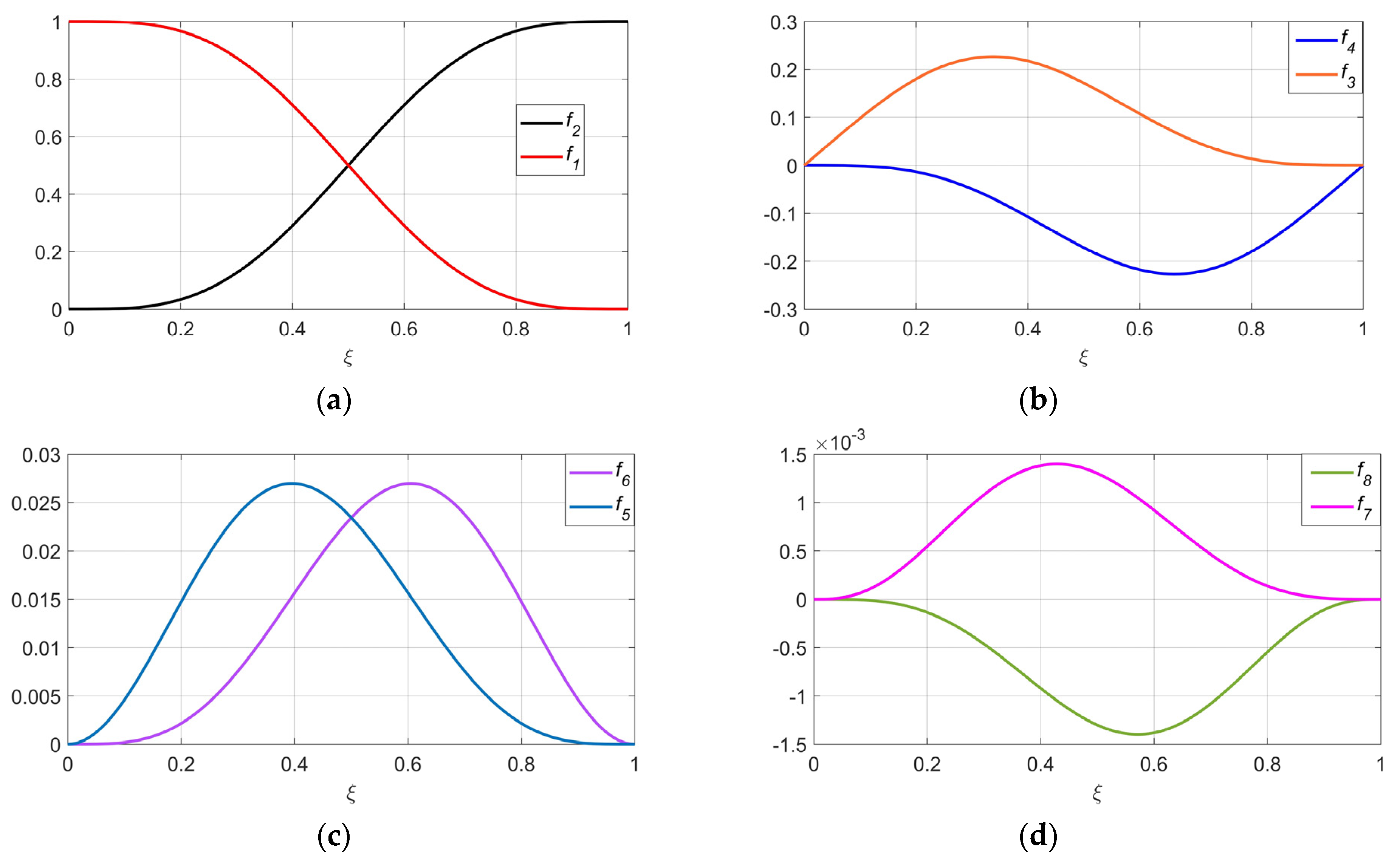
2.1. Representing Planning Parameters by Basis-Functions
2.2. One-Dimensional Quadrature Integral
2.3. SQP Nonlinear Optimization
2.4. Integral Representation of Constraints
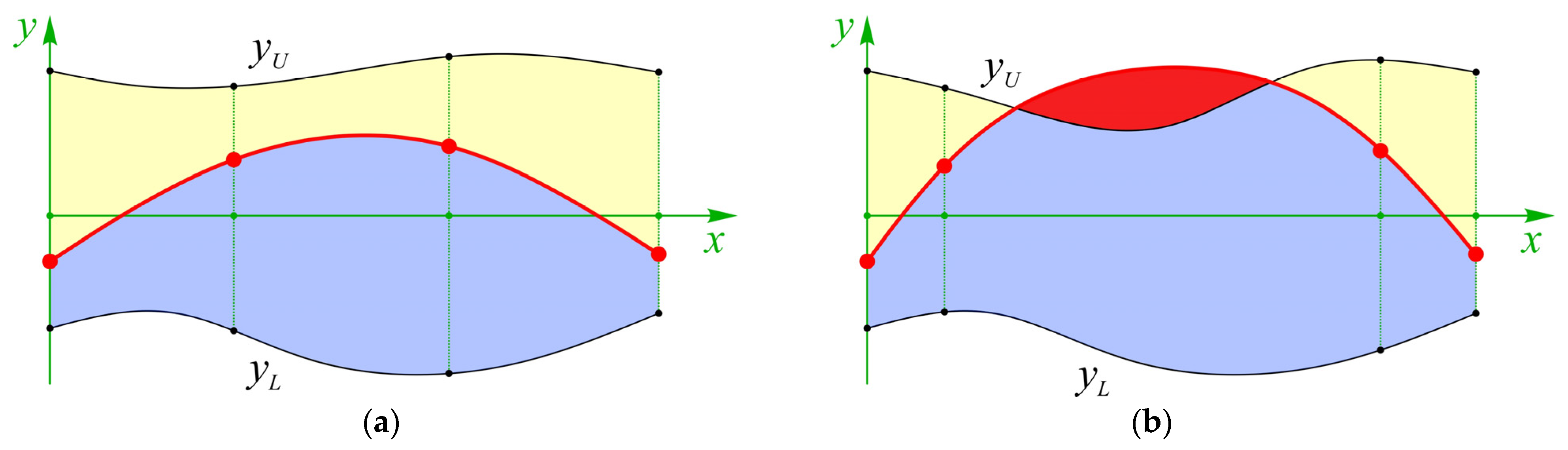
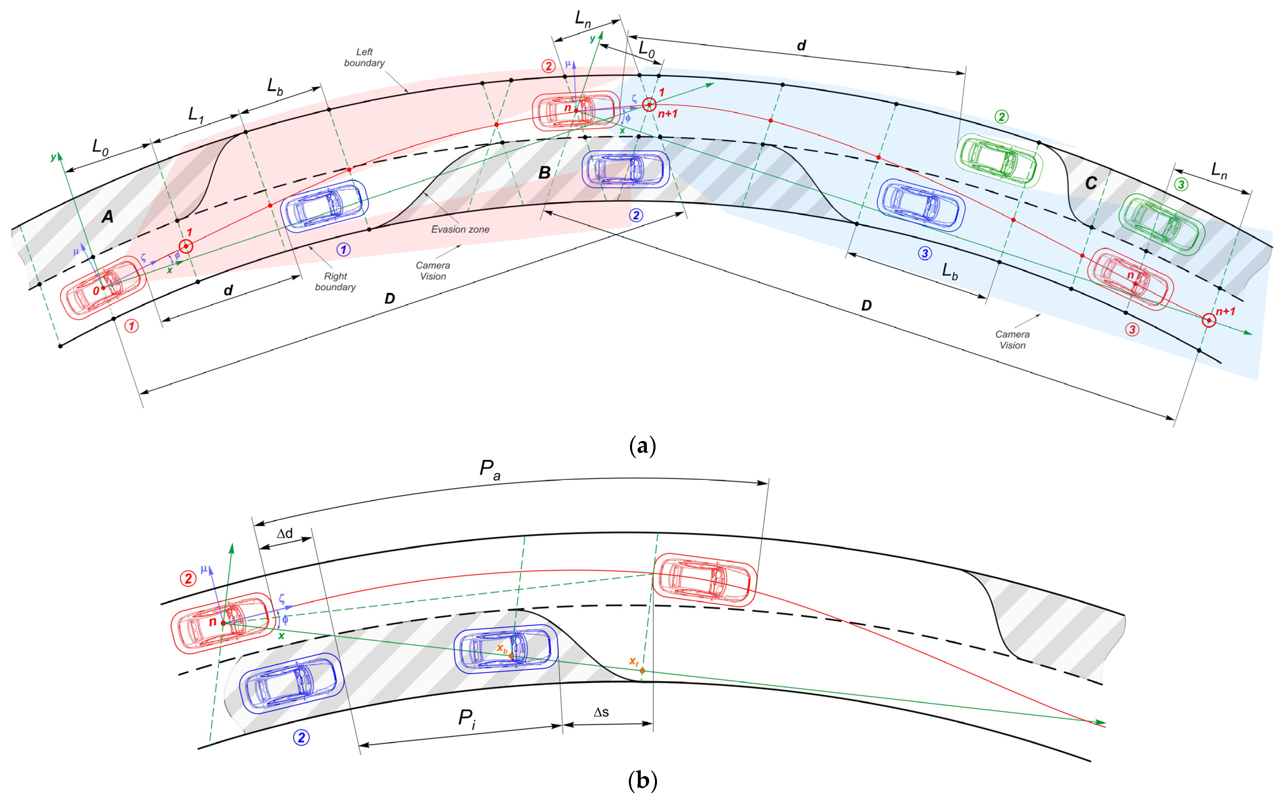
3. Technique of Planning Boundaries and Avoiding Obstacles
4. Modeling the AV Motion
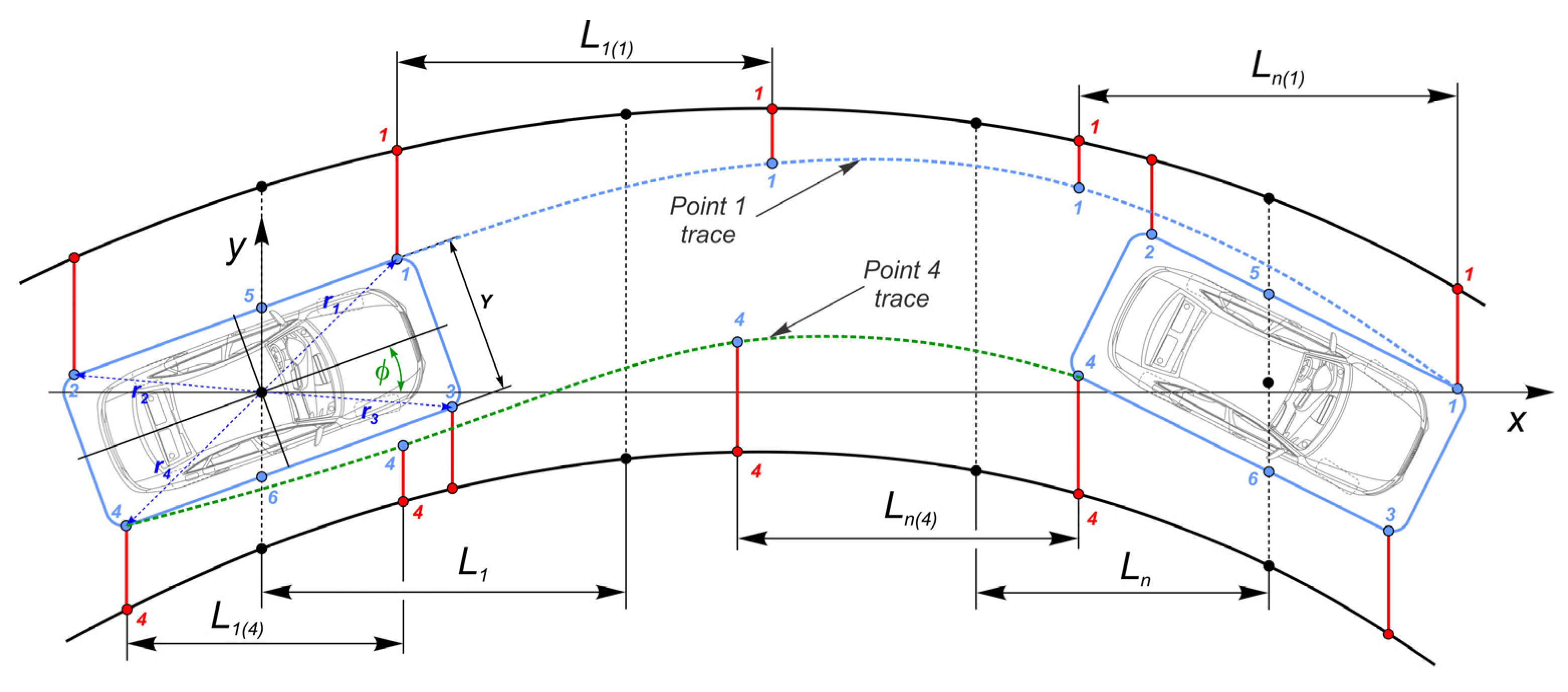
4.1. Basic Parameters of Trajectory Planning
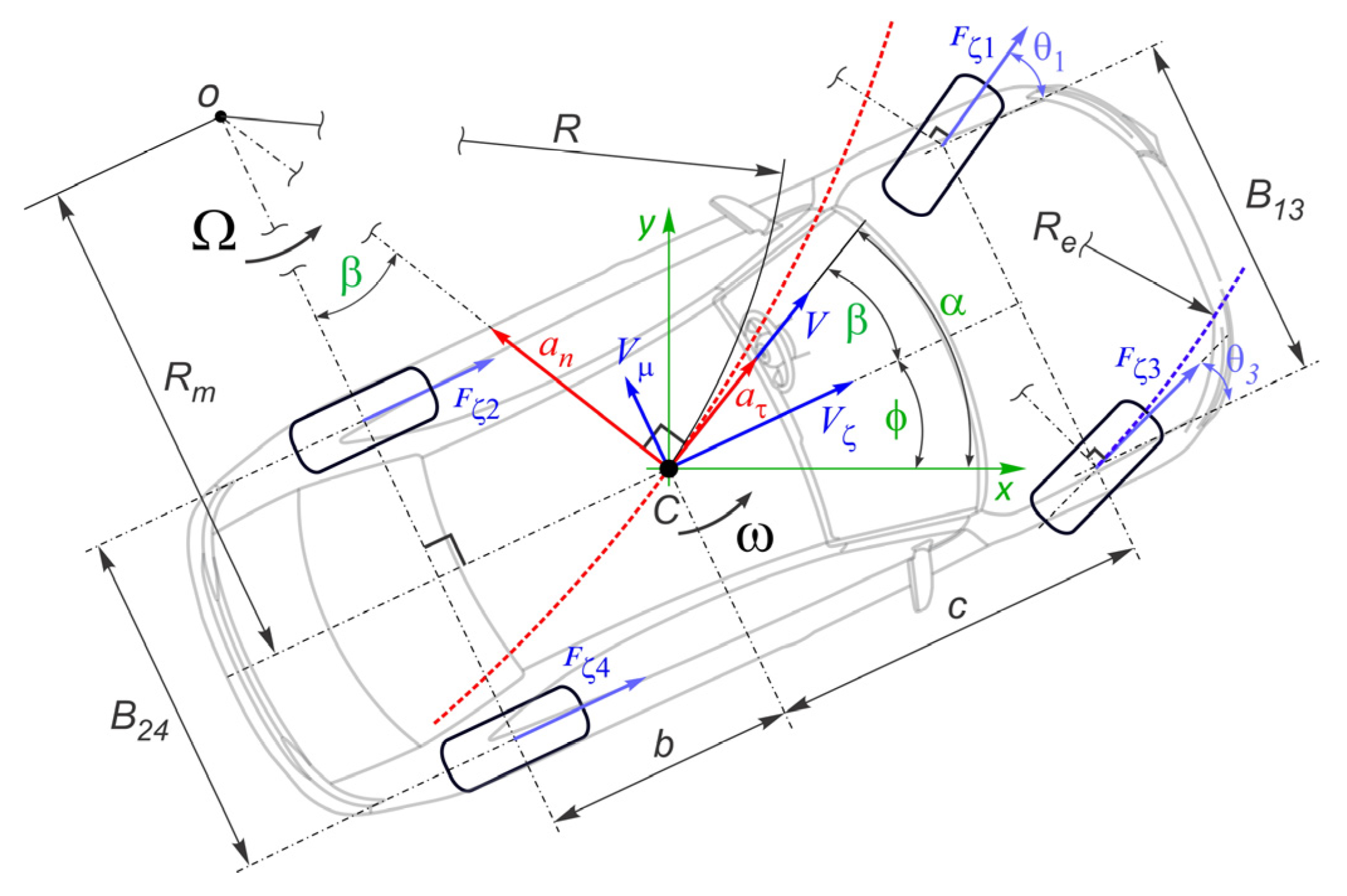
4.2. Basic Parameters of Kinematics Planning
4.3. Optimization Criteria
4.3.1. Trajectory Cost Function
4.3.2. Kinematics Cost Function
4.4. Integral Equality Constraints
4.4.1. Trajectory Restrictions
4.4.2. Physical Restrictions
4.4.3. Kinematic Restrictions
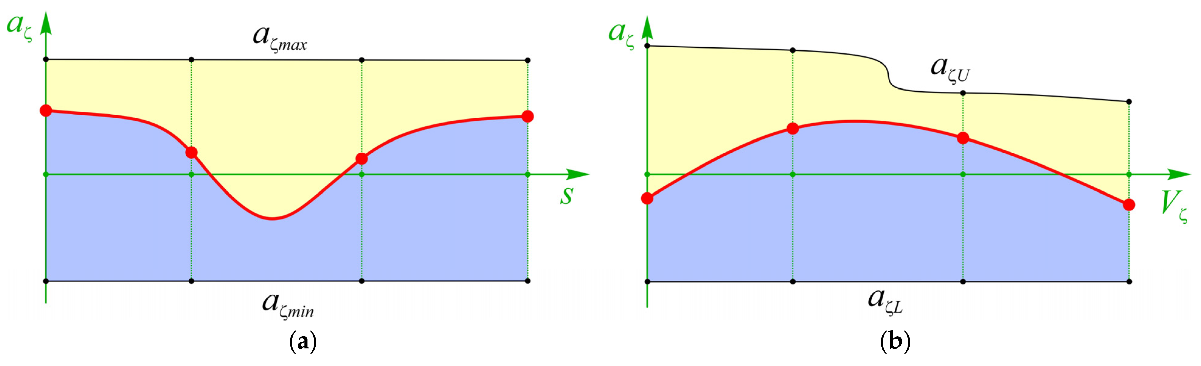
4.4.4. Dynamic Restrictions
4.4.5. Boundary Restrictions
4.5. Coordination of Transients between Phases
4.5.1. Geometric Transition Conditions
4.5.2. Kinematic Transition Conditions
4.5.3. Linear Equality Constraints
5. Simulation Example
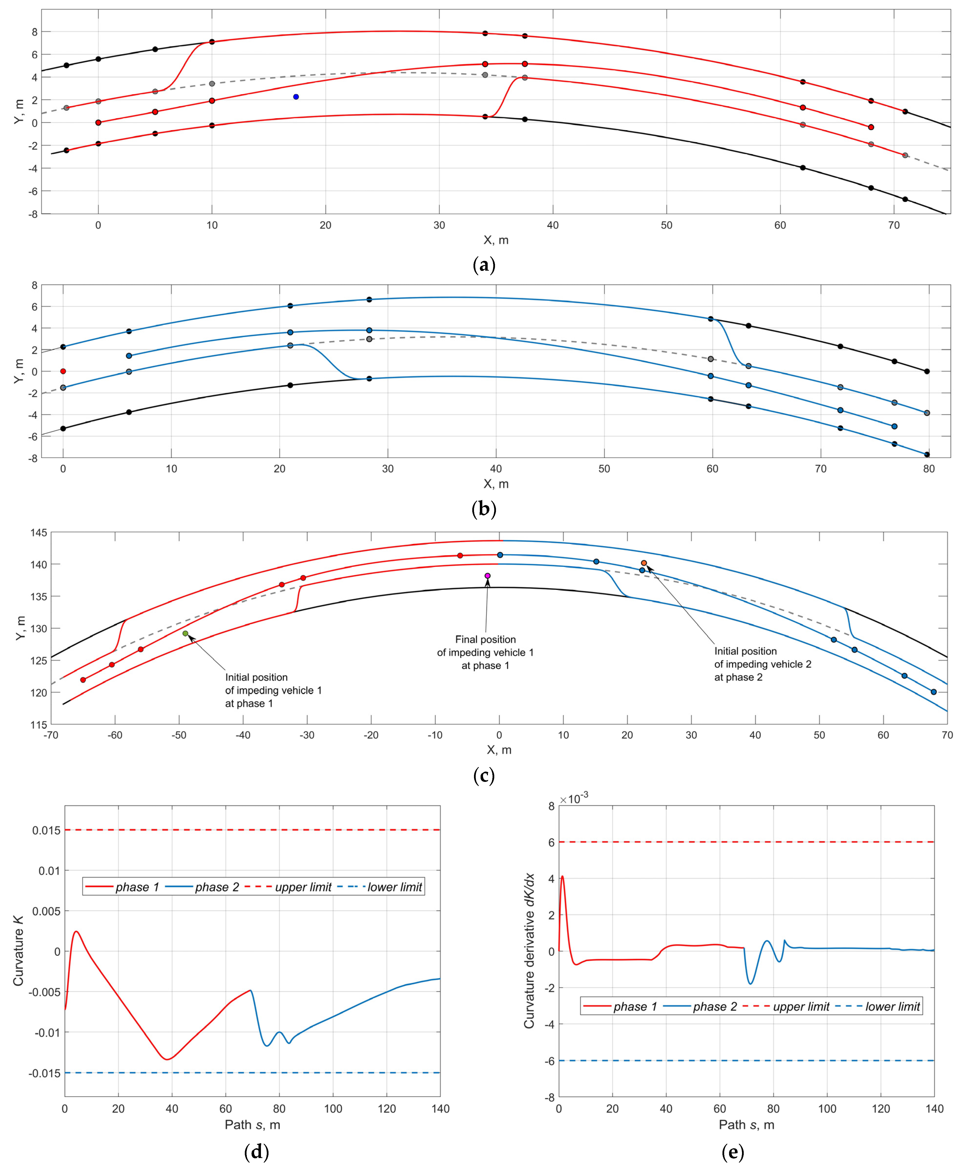
5.1. Trajectory Searching
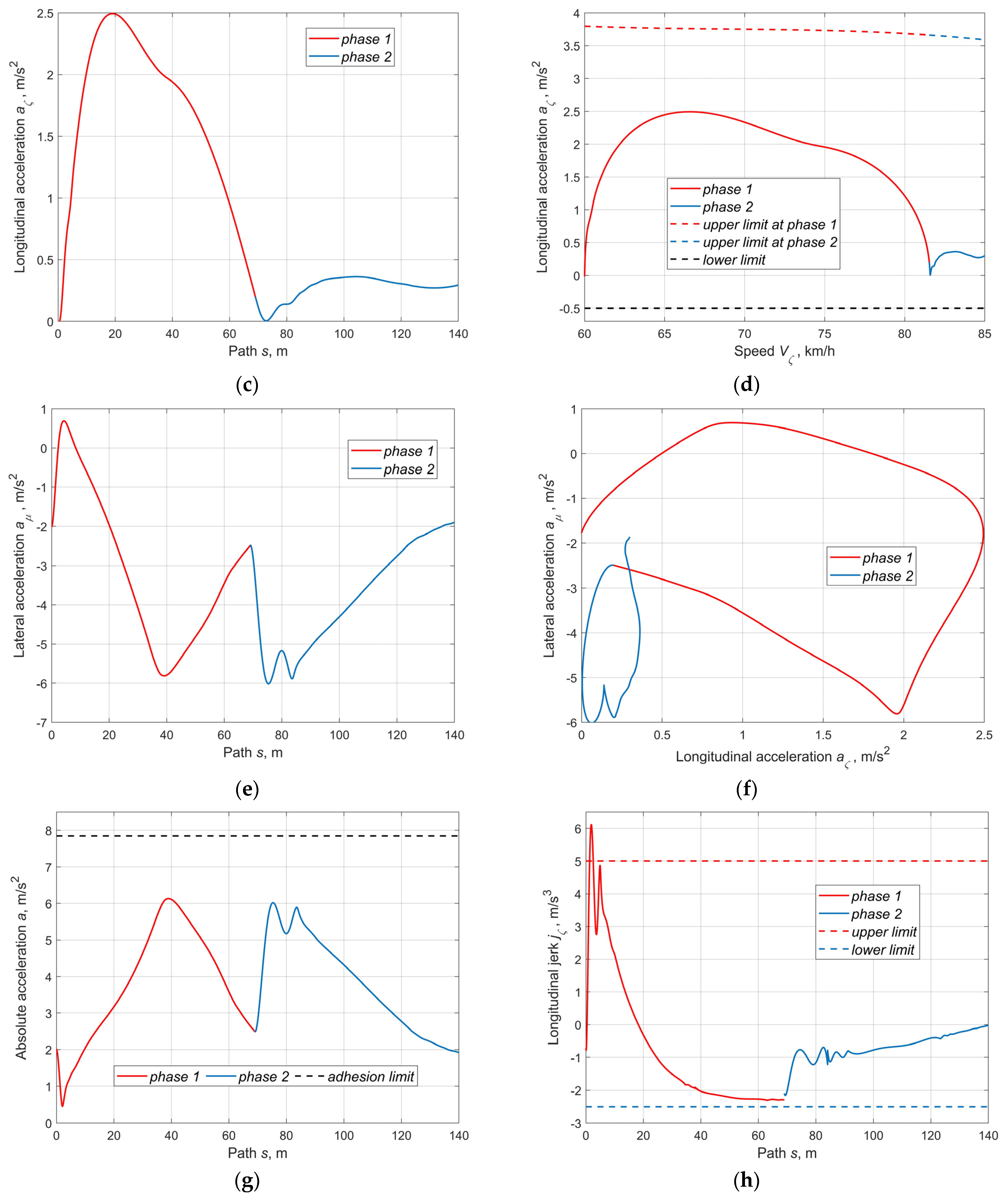
5.2. Kinematics Searching
5.3. Analysis of Results
6. Conclusions
Author Contributions
Funding
Institutional Review Board Statement
Informed Consent Statement
Data Availability Statement
Acknowledgments
Conflicts of Interest
References
- Alrifaee, B.; Scheffe, P.; Kloock, M.; Henneken, T.M. Sequential Convex Programming Methods for Real-time Trajectory Optimization in Autonomous Vehicle Racing. TechRxiv 2021. [Google Scholar] [CrossRef]
- Bautista-Camino, P.; Barranco-Gutierrez, A.I.; Cervantes, I.; Rodriguez-Licea, M.; Prado-Olivarez, J.; Perez-Pinal, F.J. Local Path Planning for Autonomous Vehicles Based on the Natural Behavior of the Biological Action-Perception Motion. Energies 2022, 15, 1769. [Google Scholar] [CrossRef]
- Chen, Y.; Ye, H.; Liu, M. Hierarchical Trajectory Planning for Autonomous Driving in Low-speed Driving Scenarios Based on RRT and Optimization. arXiv 2019, arXiv:abs/1904.02606. [Google Scholar]
- Dey, H.; Ranadive, R.; Chaudhari, A. Real-Time Trajectory and Velocity Planning for Autonomous Vehicles. Int. J. Eng. Adv. Technol. 2021, 10, 439–448. [Google Scholar] [CrossRef]
- Diachuk, M.; Easa, S.M. Motion Planning for Autonomous Vehicles Based on Sequential Optimization. Vehicles 2022, 4, 344–374. [Google Scholar] [CrossRef]
- Febbo, H.; Jayakumar, P.; Stein, J.L.; Ersal, T. Real-Time Trajectory Planning for Automated Vehicle Safety and Performance in Dynamic Environments. ASME J. Auton. Veh. Syst. 2021, 1, 041001. [Google Scholar] [CrossRef]
- Graf, M.; Speidel, O.; Dietmayer, K. Trajectory Planning for Automated Vehicles in Overtaking Scenarios. In Proceedings of the 2019 IEEE Intelligent Vehicles Symposium (IV), Paris, France, 9–12 June 2019; pp. 1653–1659. [Google Scholar] [CrossRef] [Green Version]
- Jiang, Y.; Lin, Q.; Zhang, J.; Wang, J.; Qian, D.; Cai, Y. DL-AMP and DBTO: An Automatic Merge Planning and Trajectory Optimization and its Application in Autonomous Driving. In Proceedings of the 2021 IEEE International Intelligent Transportation Systems Conference (ITSC), Indianapolis, IN, USA, 19–22 September 2021; pp. 402–409. [Google Scholar] [CrossRef]
- Li, B.; Ouyang, Y.; Li, L.; Zhang, Y. Autonomous Driving on Curvy Roads Without Reliance on Frenet Frame: A Cartesian-Based Trajectory Planning Method. IEEE Trans. Intell. Transp. Syst. 2022, 23, 15729–15741. [Google Scholar] [CrossRef]
- Li, H.; Wu, C.; Chu, D.; Lu, L.; Cheng, K. Combined Trajectory Planning and Tracking for Autonomous Vehicle Considering Driving Styles. IEEE Access 2021, 9, 9453–9463. [Google Scholar] [CrossRef]
- Lim, W.; Lee, S.; Sunwoo, M.; Jo, K. Hierarchical Trajectory Planning of an Autonomous Car Based on the Integration of a Sampling and an Optimization Method. IEEE Trans. Intell. Transp. Syst. 2018, 19, 613–626. [Google Scholar] [CrossRef]
- Liu, Y.; Zhou, B.; Wang, X.; Li, L.; Cheng, S.; Chen, Z.; Li, G.; Zhang, L. Dynamic Lane-Changing Trajectory Planning for Autonomous Vehicles Based on Discrete Global Trajectory. IEEE Trans. Intell. Transp. Syst. 2022, 23, 8513–8527. [Google Scholar] [CrossRef]
- Ma, C.; Yu, C.; Yang, X. Trajectory Planning for Connected and Automated Vehicles at Isolated Signalized Intersections under Mixed Traffic Environment. Transp. Res. Part C Emerg. Technol. 2021, 130, 103309. [Google Scholar] [CrossRef]
- Morsali, M.; Frisk, E.; Aslund, J. Deterministic Trajectory Planning for Non-Holonomic Vehicles Including Road Conditions, Safety and Comfort Factors. IFAC-PapersOnLine 2019, 52, 97–102. [Google Scholar] [CrossRef]
- Naveed, K.B.; Qiao, Z.; Dolan, J.M. Trajectory Planning for Autonomous Vehicles Using Hierarchical Reinforcement Learning. In Proceedings of the 2021 IEEE International Intelligent Transportation Systems Conference (ITSC), Indianapolis, IN, USA, 19–22 September 2021; pp. 601–606. [Google Scholar] [CrossRef]
- Nemeth, B.; Gáspár, P.; Hegedűs, T. Optimal Control of Overtaking Maneuver for Intelligent Vehicles. J. Adv. Transp. 2018, 2018, 2195760. [Google Scholar] [CrossRef]
- Peng, T.; Su, L.; Guan, Z.; Hou, H.; Li, J.; Liu, X.; Tong, Y. Lane-Change Model and Tracking Control for Autonomous Vehicles on Curved Highway Sections in Rainy Weather. J. Adv. Transp. 2020, 2020, 8838878. [Google Scholar] [CrossRef]
- Peng, B.; Yu, D.; Zhou, H.; Xiao, X.; Xie, C. A Motion Planning Method for Automated Vehicles in Dynamic Traffic Scenarios. Symmetry 2022, 14, 208. [Google Scholar] [CrossRef]
- Said, A.; Talj, R.; Francis, C.; Shraim, H. Local trajectory planning for autonomous vehicle with static and dynamic obstacles avoidance. In Proceedings of the 2021 IEEE International Intelligent Transportation Systems Conference (ITSC), Indianapolis, IN, USA, 19–22 September 2021; pp. 410–416. [Google Scholar] [CrossRef]
- Scheffe, P.; Dorndorf, G.; Alrifaee, B. Increasing Feasibility with Priority Assignment in Distributed Trajectory Planning for Road Vehicles. TechRxiv 2022. [Google Scholar] [CrossRef]
- Sun, K.; Zhao, X.; Wu, X. A cooperative lane change model for connected and autonomous vehicles on two lanes highway by considering the traffic efficiency on both lanes. Transp. Res. Interdiscip. Perspect. 2021, 9, 100310. [Google Scholar] [CrossRef]
- Van Hoek, R.; Ploeg, J.; Nijmeijer, H. Cooperative Driving of Automated Vehicles Using B-Splines for Trajectory Planning. IEEE Trans. Intell. Veh. 2021, 6, 594–604. [Google Scholar] [CrossRef]
- Wang, A.; Jasour, A.; Williams, B. Non-Gaussian Chance-Constrained Trajectory Planning for Autonomous Vehicles Under Agent Uncertainty. IEEE Robot. Autom. Lett. 2020, 5, 6041–6048. [Google Scholar] [CrossRef]
- Wang, Y.; Wei, C. A Universal Trajectory Planning Method for Automated Lane-Changing and Overtaking Maneuvers. Math. Probl. Eng. 2020, 2020, 1023975. [Google Scholar] [CrossRef]
- Wei, C.; Li, S. Planning a Continuous Vehicle Trajectory for an Automated Lane Change Maneuver by Nonlinear Programming considering Car-Following Rule and Curved Roads. J. Adv. Transp. 2020, 2020, 8867447. [Google Scholar] [CrossRef]
- Xin, L.; Kong, Y.; Li, S.E.; Chen, J.; Guan, Y.; Tomizuka, M.; Cheng, B. Enable faster and smoother spatio-temporal trajectory planning for autonomous vehicles in constrained dynamic environment. Proc. Inst. Mech. Eng. Part D J. Automob. Eng. 2021, 235, 1101–1112. [Google Scholar] [CrossRef]
- Yuan, C.; Wei, Y.; Shen, J.; Chen, L.; He, Y.; Weng, S.; Wang, T. Research on path planning based on new fusion algorithm for autonomous vehicle. Int. J. Adv. Robot. Syst. 2020, 17, 1729881420911235. [Google Scholar] [CrossRef]
- Varvak, P.M. Finite Element Method: Textbook for High Schools; Kyiv—Higher School, Head Publishing House: Kyiv, Ukraine, 1981; 176p. [Google Scholar]
- Grishkevich, A.I. Automobiles: Theory: Textbook for high schools. Minsk High Sch. 1986, 208, 431–438. [Google Scholar]
- Pacejka, H.B. Tire and Vehicle Dynamics, 3rd ed.; Elsevier: Oxford, UK, 2012. [Google Scholar]
- MATLAB R2021b. Available online: https://www.mathworks.com/ (accessed on 20 June 2022).


| Ref. | Path Model | Speed Model | Optimization Model | Constraints |
|---|---|---|---|---|
| [1] | The track circuit represents the allowable driving area; the center line is the reference; the forward vector is defined by the gradient of the center-line | No yaw is considered; the vehicle is facing in the same direction as the longitudinal velocity; the speed is determined based on the control of accelerations | MPC as the control structure; General Trajectory Optimization Problem: the goal is to maximize the track progression; sequential convex programming methods; sequential linearization | The left and right boundary points along the normal direction with the track width; linearized non-convex constraints of the optimization problem |
| [2] | Free collision trajectory; local path planner based on Vehicle Attractor Dynamic Approach (VADA) | Lateral vehicle dynamic model; single-track model with seven DOF | Control vector is formed by the steering angle rate and by the longitudinal acceleration; PID controller for the vehicle speed determines the throttle and brake pedal positions | Ranges of the maximum lateral and longitudinal accelerations; maximum speed |
| [3] | Cubic-curvature curves; modified bidirectional rapidly exploring random tree (bi-RRT) approach | Discrete speed model based on the final differences of the path curve | Feasible online SQP to minimize the time and acceleration costs | Limited curvature, time, speed, acceleration, kinematic constraints |
| [4] | Cubic splines connecting three path nodes situated at equal distances between the initial and the target point | Trapezoidal velocity profile; interpolating cubic polynomials for parameterization of the velocity profile | Band Matrix Method to find the path model variables. The trapezoidal velocity profile is smoothened to guarantee the acceleration continuity. Minimum travel time through the specified path | Lane constraints, speed limit 50 MPH, acceleration limit 10 m/s2, jerk limit 10 m/s3, initial and final velocity |
| [5] | Trajectory is combined of finite elements represented by the nodal DOF and basis functions based on the 5th order polynomial | FE model with 3 DOF in a node to ensure the jerk continuity; kinematic vehicle model with ideal turn | Sequential nonlinear optimization of trajectory and speed with nonlinear constraints; SQP method; curvature rate and slip angle as basic criteria for trajectory cost function; speed deviation, longitudinal acceleration and jerk are basic criteria for the speed profile cost function | Allowable motion zone with boundaries; critical slip speed, maximum acceleration by the powertrain properties, maximum adhesion, initial and final conditions |
| [6] | Trajectory is formed by the longitudinal and lateral displacements to avoid a set of obstacles between the initial and target locations | 3 DOF vehicle model; system of 8 state-space differential equations including controls; | Nonlinear model predictive control framework for non-negligible optimal control problem (OCP); cost function criteria include: vehicle’s global position coordinates, steering angle, steering rate, longitudinal jerk, and parameters to prevent the minimum vertical tire load | State bounds: longitudinal and lateral displacements, yaw angle, steering angle, longitudinal speed and acceleration; control restrictions: steering rate, longitudinal jerk |
| [7] | Road structure is represented by the center lines of the adjacent lanes relevant for overtaking | Constant velocity model within the Kalman filter | SQP-method to optimize the cost function based on deviation from the reference trajectory, acceleration and jerk | Probabilistic forbidden zones; maximum lateral acceleration, limited steering angle, spatial constraints to make |
| [8] | Fifth degree polynomial trajectory generation method; single trajectory instead of piecewise | Fifth degree polynomial trajectory generation method | Two stages of constrained quadratic programming (QP); gradient based method that considers trajectory smoothness and curvature; cost function to evaluate efficiency, comfort, and safety consists of steady state relative distance, time to collision, total time, and acceleration | The sampling time range is between 4.5 s and 7.0 s; maximum trajectory curvature, maximum absolute value of offset between original trajectory and smoothed trajectory |
| [9] | Reference trajectory refers to a coarse trajectory; a reference trajectory is derived by searching an abstracted state space via dynamic programming (DP) | Speed is integrated as a state element in the Cartesian frame based on the jerk as a control parameter | Optimal control problem (OCP) is solved numerically via a gradient-based optimizer; the cost function is represented by deviations from reference trajectory (linear and angular coordinates), and control profiles towards zero (jerk and yaw rate) | Collision avoidance constraints; allowable bounds of the state/control profiles: maximum acceleration, speed, jerk, yaw rate, yaw angle |
| [10] | The combined trajectory planning and tracking method; vehicle moves forward along the lane with the longitudinal and lateral potentials | Speed is calculated from the vehicle kinematics model | MPC and Artificial Potential Field (APF); APF for environment, local vehicle, and driving style as parts of the objective function | The desired speed, maximum acceleration, limits of the controls and their increments; current lane boundary restrictions |
| [11] | Behavioral trajectory planning in three steps: path candidate generation, optimal speed profile generation, and trajectory selection; converting behavioral trajectory into a denser trajectory | Path-velocity decomposition method; spatiotemporal nodes; two steps: the speed limit profile generation and the optimal speed search determined by the maximum lateral acceleration | Numerical optimization for motion trajectory planning; objective function: reference cost, acceleration, jerk calculated by the final differences; basic SQP performs optimization by approximating the objective function using second-order differentiation | Speed limits, maximum vehicle acceleration, environment constraints, avoidance of collisions with dynamic objects constraints |
| [12] | Cubic polynomial for smooth curve of lateral offset depending on the path length | Cubic polynomial for the planned speed as function of the path length | Three criteria in terms of efficiency, comfort and safety are adopted to compose the cost function | Road speed limit, yaw rate, maximum and minimum accelerations |
| [13] | Bi-level optimization the trajectory planning; the prediction is based on current traffic conditions and vehicle driving behaviors determined by car-following and lane-changing models; lane-changing strategy tree | Second-order vehicle kinematics; speed distribution based on the acceleration profile optimization | The upper-level optimization minimizes the overall cost including travel time, fuel consumption, and lane-changing cost; the lower-level optimization determines the optimal acceleration for minimum travel time and fuel consumption by the given trajectory from the upper-level model | Distance between preceding and following vehicles; the minimum time interval between two consecutive lane-changing maneuvers; absolute values of the maximum deceleration (4 m/s2) and acceleration (2 m/s2) |
| [14] | For path planning any method can be used | The speed planner updates the path information by evaluating conditions and vehicle status, the planner calculates a speed profile based on longitudinal acceleration and jerk. | A minimum time optimization control problem; the optimal speed profile ensures a safe and comfortable vehicle speed for the is obtained. | Rollover criterion, maximum speed corresponding to the maximum lateral acceleration, skidding friction, steering rate, steer angle, maximum acceleration and jerk |
| [15] | Two high-level options (lane follow/wait and lane change); waypoint on the target-lane is selected using the ego-vehicle state information through the epsilon greedy strategy; sub-trajectories form a complete trajectory | Target speed is calculated using the maximum acceleration or deceleration to ensure a smooth sub-trajectory; then the target speed and final waypoint values are given, the PID controller generates longitudinal and lateral control | Double Q-Learning; deep Q-Learning algorithm is used to find an optimal action-selection policy to maximize the action-value function through minimizing the loss function between predicted action-value and the target action-value | Regular time step penalty, regular time step reward for progressing towards final destination, collision penalty, unsafe penalty, goal not required penalty, non-smoothness penalty, Success Reward |
| [16] | Trajectory design is based on a constrained optimization; clothoid trajectory for the lateral displacement and yaw angle | Kinematic equations for the longitudinal velocity and displacement for planning; vehicle is described by the dynamical bicycle model for tracking | Minimizing the tracking error and the ratios of the clothoid sections by a quadratic programming method; LPV-based control design method to guarantee the tracking of the generated trajectory | Finite horizon length; constraints are incorporated into the trajectory optimization problem; minimum and maximum lateral offsets |
| [17] | Quadratic time-based function for longitudinal displacement; 4th extent time depending function for lateral displacement | Linear time depending function for the vehicle longitudinal velocity; Gaussian distribution for describing the vehicle lateral velocity | MPC is converted to a standard quadratic programming problem; nonlinear vehicle dynamic model is linearized as a linear time invariant (LTI) state space form | Vehicle state and control constraints; maximum acceleration, road adhesion limit |
| [18] | Cubic spline interpolation to find the driving centerline points in the Cartesian coordinate system from sampling points of the Frenet frame; quintic time depending polynomial for lateral and longitudinal displacement | Fourth extent polynomials for the lateral and longitudinal velocities; 3th extent polynomials for the lateral and longitudinal accelerations | The cost function considers the longitudinal and lateral jerks, offset degree from the reference line, deviation between the planning and desired speeds, minimum distance between the AV and the obstacles, cost of a collision between the AV and the static or dynamic obstacles | Lateral position sampling range; predicted time sampling range; target speed sampling range; predicted time sampling interval; target speed sampling interval |
| [19] | Reference map; candidate paths in the curvilinear coordinate system; 4th order polynomial for the lateral offset | Desired velocity profile based on a set of speed limitations | Objective function includes the factors such as smoothness, consistency, reference tracking and safety | Prediction horizon; speed is restricted by imposing the lateral acceleration limitation |
| [20] | Path-velocity decomposition; the path is treated as an input | Double integrator model for the movement along the path; the model yields the agent’s position from its velocity and acceleration | Velocity is optimized to follow a reference by solving the optimal control problem (OCP) | Constraints: input, states, terminal position, prediction horizon |
| [21] | Independent movements in lateral and longitudinal directions; the sine function curve is applied to determine the trajectory; lane change in original lane (LC-O) stage and lane change in target lane (LC-T) | Velocity and acceleration in the lateral direction of lane change are obtained by the first and second derivatives of the trajectory curve model | Cost function is designed to optimize processes of LC-O stage and LC-T stage; objective functions represent desired accelerations at the LC-O stage and LC-T stages, the gap errors between vehicles, and the terminal cost | Maximum longitudinal and lateral accelerations, safe gap constraint at critical moment, gap of host vehicle and surrounding vehicles, the minimum time |
| [22] | A set of possible trajectories based on B-splines; quintic polynomials to connect initial state with a grid of terminal constraints in space and time dimensions | The first-order dynamics for the vehicle driveline based on the longitudinal acceleration, commanded acceleration, and time constant; virtual triple integrator system | The cost function selects the optimal (feasible and collision free) trajectory from the generated set by minimizing the cumulative error in the B-spline over the entire prediction horizon | Testing possible violations of constraints and occurrence of collisions; Schoenberg-Whitney’s Condition; constant zero acceleration for the extended trajectory |
| [23] | Third order polynomials to independently represent x and y displacement | Kinematic bicycle model to calculate state vector including velocity | Chance-constrained model predictive control (cc-MPC); model predictive contouring control cost function penalizing contouring deviation, lag error, control effort, and deviation from a reference speed | Chance-constraint enforced with deterministic nonlinear constraints; upper bounds on the probability of violating constraints using Cantelli’s inequality |
| [24] | Quintic polynomial for the lateral offset as function of longitudinal displacement; longitudinal position, lateral position, derivative, and the curvature of the lane curve to find the polynomial coefficients | Speed, acceleration, and jerk profiles are based on the quintic polynomial of the driving distance profile over time | Objective function of the constrained nonlinear optimization model containing acceleration and jerk of the ego vehicle, and the total driving time | Collision-avoidance constraints; maximum total time, speed, acceleration, and jerk; traffic state constraint |
| [25] | Sixth order time depending polynomial functions for the longitudinal and lateral positions | The speed kinematic model is represented by the time quadratic equation with acceleration and jerk; kinematic variables: longitudinal and lateral positions, accelerations, jerks | SQP algorithm to solve the nonlinear programming by minimizing the longitudinal and lateral accelerations and jerks, and time, the safety risk and discomfort for vehicle | Restricted distances between vehicles, constraints for the longitudinal and lateral speeds, accelerations, jerks, and horizon time |
| [26] | Three-dimensional spatio-temporal driving map; reference trajectory generation with a search-based method, followed by local refinement and smoothing | Vehicle states are: the lateral and longitudinal positions, velocity, and yaw angle; the action space includes possible acceleration and yaw angle | Time-invariant MPC extended by the reconstruction of convex feasible sets; objective function includes parameters: prediction horizon time, initial position, target destination, reference state of the spatio-temporal trajectory, control input | State constraints for each state; limits of control input; deviation of longitudinal velocity from the desired value with the limit of 20 m/s |
| [27] | Path is searched by ant colony algorithm according to the path enlightened by artificial potential field algorithm | Vehicle accelerates to reach speed of 80 km/h, deceleration to 40 km/h; vehicle travels at speed of 30, 50, and 100 km/h | Transfer probability function of ant colony algorithm, improved potential field algorithm; gravity model of safety lane change | Speed limits of front section 80 and 40 km/h;lateral acceleration changes from −0.15 g to 0.15 g |
| Parameter | Value | Parameter | Value | Parameter | Value |
|---|---|---|---|---|---|
| c, [m] | 1.43 | m, [kg] | 1960 | ρa, [kg/m3] | 1.225 |
| b, [m] | 1.37 | ϕmax | 0.8 | Cx | 0.24 |
| Y, [m] | 1.551 | Vζmax, [km/h] | 85 | Af, [m2] | 2.04 |
| |rζk|, [m] | 2.5 | Vζ (0), [km/h] | 60 | D, [m] | 67.98/76.8 |
| |rμk|, [m] | 1.2 | n | 6 | d, [m] | 17.5/ 21.5 |
Publisher’s Note: MDPI stays neutral with regard to jurisdictional claims in published maps and institutional affiliations. |
© 2022 by the authors. Licensee MDPI, Basel, Switzerland. This article is an open access article distributed under the terms and conditions of the Creative Commons Attribution (CC BY) license (https://creativecommons.org/licenses/by/4.0/).
Share and Cite
Diachuk, M.; Easa, S.M. Improved Technique for Autonomous Vehicle Motion Planning Based on Integral Constraints and Sequential Optimization. Vehicles 2022, 4, 1122-1157. https://doi.org/10.3390/vehicles4040060
Diachuk M, Easa SM. Improved Technique for Autonomous Vehicle Motion Planning Based on Integral Constraints and Sequential Optimization. Vehicles. 2022; 4(4):1122-1157. https://doi.org/10.3390/vehicles4040060
Chicago/Turabian StyleDiachuk, Maksym, and Said M. Easa. 2022. "Improved Technique for Autonomous Vehicle Motion Planning Based on Integral Constraints and Sequential Optimization" Vehicles 4, no. 4: 1122-1157. https://doi.org/10.3390/vehicles4040060
APA StyleDiachuk, M., & Easa, S. M. (2022). Improved Technique for Autonomous Vehicle Motion Planning Based on Integral Constraints and Sequential Optimization. Vehicles, 4(4), 1122-1157. https://doi.org/10.3390/vehicles4040060