
Motion Planning for Autonomous Vehicles Based on Sequential Optimization


Abstract
:1. Introduction
2. Generalization of Mathematical Tools
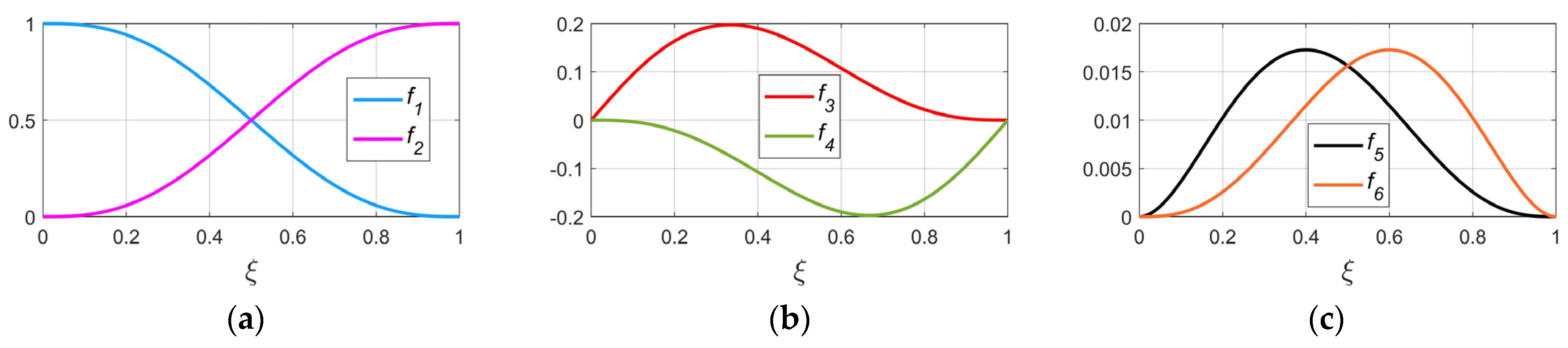
2.1. Representing the Parameters of Planning Functions by Finite Elements
2.2. Nonlinear Optimization
3. Trajectory Search
3.1. Problem Generalization
3.2. Description of Trajectory Planning Objective
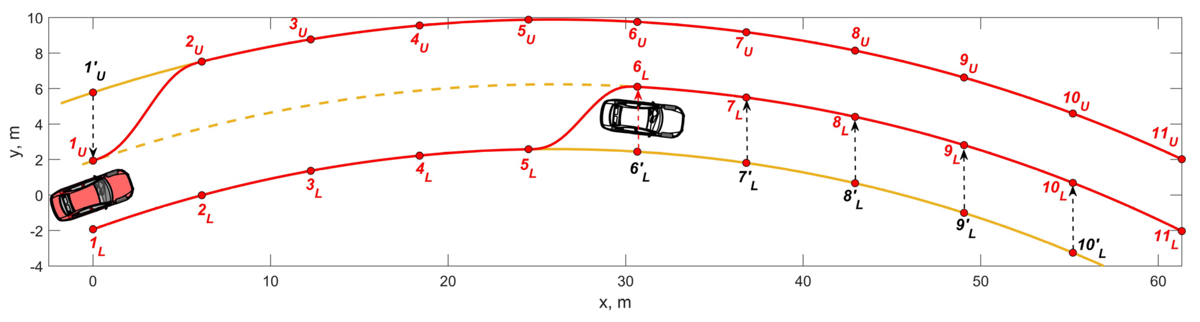
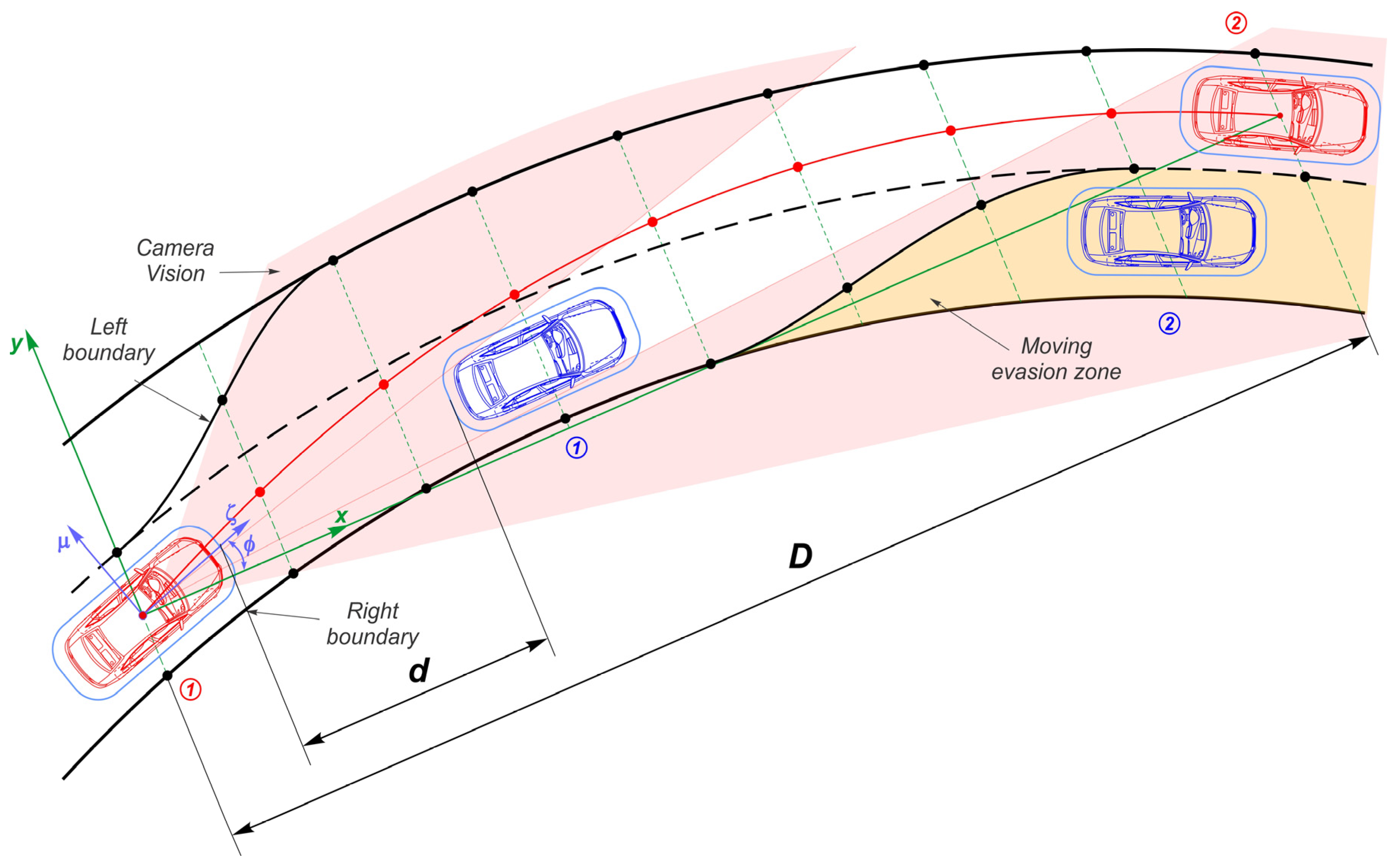
3.3. Determining the Maneuver Boundaries
3.4. Trajectory Geometry
3.5. Cost Functions
3.6. Constraints
3.6.1. Dimensional Constraints
3.6.2. Other Constraints
4. Searching Distributions of Kinematic Parameters
4.1. Problem Generalization
4.2. Kinematic Parameters and Their Derivatives
4.3. Objective Functions
4.4. Optimal Kinematics Restrictions
4.4.1. Slip Critical Speed
4.4.2. Linear Inequality Constraints
4.4.3. Linear Equality Constraints
4.4.4. Vehicle Maximum Performance
4.5. Initial Conditions
5. Simulation Example
5.1. Trajectory Search
5.2. Speed Search
5.3. Results
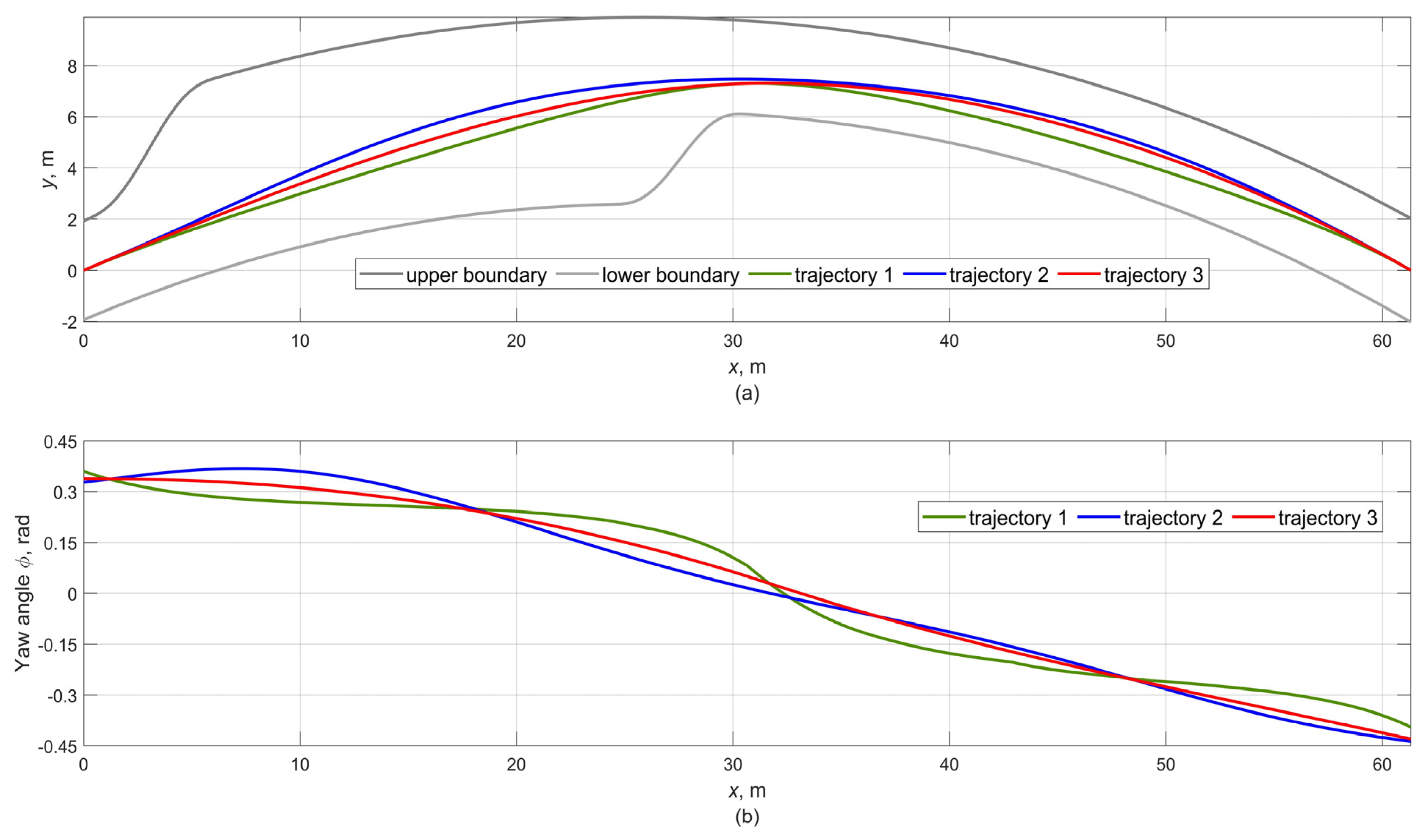
5.3.1. Trajectories
5.3.2. Speed and Accelerations
5.3.3. Satisfaction of Physical Constraints
5.3.4. Weighting Coefficients and Their Influence
6. Conclusions
- the approach combines the advantages of representing solutions by FEs and nonlinear optimization;
- the technique for limiting allowable space was considered;
- the complete mathematical apparatus was developed providing clear connections between geometric and kinematic parameters in the spatial domain, which abolishes the need for setting a time of prediction horizon;
- geometric restrictions are clearly defined in the form of nonlinear constraints, which guarantees the vehicle location within the boundaries;
- the kinematic parameters are strictly interconnected, which is shown in the formulas for acceleration and sharpness unlike other works;
- the distribution of speed and accelerations is performed directly along the trajectory without reference to time and provides natural smooth curves in contrast to the speed representation as a time function based on 2nd- or 3rd-degree polynomials proposed in many works. In this case, the acceleration and jerk are considered only along the longitudinal coordinate and are often assigned as either linear or constant, which does not reflect the real nature of the propulsion system operation;
- all the necessary procedures (unlike other works) for implementing the method in the computer simulation environment are reflected.
Author Contributions
Funding
Institutional Review Board Statement
Informed Consent Statement
Data Availability Statement
Acknowledgments
Conflicts of Interest
References
- Claussmann, L.; Revilloud, M.; Gruyer, D.; Glaser, S. A Review of Motion Planning for Highway Autonomous Driving. IEEE Trans. Intell. Transp. Syst. 2019, 21, 1826–1848. [Google Scholar] [CrossRef] [Green Version]
- Piazzi, A.; Bianco, C.G.L.; Romano, M. μ3-Splines for the Smooth Path Generation of Wheeled Mobile Robots. IEEE Trans. Robot. 2007, 23, 1089–1095. [Google Scholar] [CrossRef]
- Villagra, J.; Milanes, V.; Pérez, J.; Godoy, J. Smooth path and speed planning for an automated public transport vehicle. Robot. Auton. Syst. 2012, 60, 252–265. [Google Scholar] [CrossRef]
- Andersen, H.; Schwarting, W.; Naser, F.; Eng, Y.H.; Ang, M.H.; Rus, D.; Alonso-Mora, J. Trajectory optimization for autonomous overtaking with visibility maximization. In Proceedings of the IEEE 20th International Conference on Intelligent Transportation Systems (ITSC), Yokohama, Japan, 16–19 October 2017; pp. 1–8. [Google Scholar] [CrossRef]
- Liu, C.; Lee, S.; Varnhagen, S.; Tseng, H.E. Path planning for autonomous vehicles using model predictive control. In Proceedings of the IEEE Intelligent Vehicles Symposium (IV), Los Angeles, CA, USA, 11–14 June 2017; pp. 174–179. [Google Scholar] [CrossRef]
- Raksincharoensak, P.; Hasegawa, T.; Nagai, M. Motion Planning and Control of Autonomous Driving Intelligence System Based on Risk Potential Optimization Framework. Int. J. Automot. Eng. 2016, 7, 53–60. [Google Scholar] [CrossRef] [Green Version]
- McNaughton, M.; Urmson, C.; Dolan, J.; Lee, J.-W. Motion planning for autonomous driving with a conformal spatiotemporal lattice. In Proceedings of the 2011 IEEE International Conference on Robotics and Automation, Shanghai, China, 9–13 May 2011; pp. 4889–4895. [Google Scholar] [CrossRef]
- Artunedo, A.; Villagra, J.; Godoy, J. Real-Time Motion Planning Approach for Automated Driving in Urban Environments. IEEE Access 2019, 7, 180039–180053. [Google Scholar] [CrossRef]
- Typaldos, P.; Papageorgiou, M.; Papamichail, I. Optimization-based path-planning for connected and non-connected automated vehicles. Transp. Res. Part C Emerg. Technol. 2021, 134, 103487. [Google Scholar] [CrossRef]
- Altché, F.; Polack, P.; de La Fortelle, A. High-speed trajectory planning for autonomous vehicles using a simple dynamic model. In Proceedings of the 2017 IEEE 20th International Conference on Intelligent Transportation Systems (ITSC), Yokohama, Japan, 16–19 October 2017; pp. 1–7. [Google Scholar] [CrossRef] [Green Version]
- Talamino, J.P.; Sanfeliu, A. Anticipatory kinodynamic motion planner for computing the best path and velocity trajectory in autonomous driving. Robot. Auton. Syst. 2018, 114, 93–105. [Google Scholar] [CrossRef]
- El Mahdawy, A.; El Mougy, A. Path Planning for Autonomous Vehicles with Dynamic Lane Mapping and Obstacle Avoidance. In Proceedings of the 13th International Conference on Agents and Artificial Intelligence, Online Streaming, 4–6 February 2021; pp. 431–438. [Google Scholar] [CrossRef]
- Katrakazas, C.; Quddus, M.; Chen, W.-H.; Deka, L. Real-time motion planning methods for autonomous on-road driving: State-of-the-art and future research directions. Transp. Res. Part C Emerg. Technol. 2015, 60, 416–442. [Google Scholar] [CrossRef]
- Kuwata, Y.; Fiore, G.A.; Teo, J.; Frazzoli, E.; How, J.P. Motion planning for urban driving using RRT. In Proceedings of the IEEE/RSJ International Conference on Intelligent Robots and Systems, Nice, France, 22–26 September 2008; pp. 1681–1686. [Google Scholar] [CrossRef] [Green Version]
- Chen, J.; Zhang, R.; Han, W.; Jiang, W.; Hu, J.; Lu, X.; Liu, X.; Zhao, P. Path Planning for Autonomous Vehicle Based on a Two-Layered Planning Model in Complex Environment. J. Adv. Transp. 2020, 2020, 1–14. [Google Scholar] [CrossRef]
- Gu, T.; Atwood, J.; Dong, C.; Dolan, J.M.; Lee, J.-W. Tunable and stable real-time trajectory planning for urban autonomous driving. In Proceedings of the IEEE/RSJ International Conference on Intelligent Robots and Systems (IROS), Hamburg, Germany, 28 September–2 October 2015; pp. 250–256. [Google Scholar] [CrossRef]
- Kapania, N.R.; Subosits, J.; Gerdes, J.C. A Sequential Two-Step Algorithm for Fast Generation of Vehicle Racing Trajectories. J. Dyn. Syst. Meas. Control 2016, 138, 091005. [Google Scholar] [CrossRef] [Green Version]
- Medina-Lee, J.; Artuñedo, A.; Godoy, J.; Villagra, J. Merit-Based Motion Planning for Autonomous Vehicles in Urban Scenarios. Sensors 2021, 21, 3755. [Google Scholar] [CrossRef] [PubMed]
- Morsali, M.; Frisk, E.; Åslund, J. Deterministic Trajectory Planning for Non-Holonomic Vehicles Including Road Conditions, Safety and Comfort Factors. IFAC-PapersOnLine 2019, 52, 97–102. [Google Scholar] [CrossRef]
- Subosits, J.K.; Gerdes, J.C. From the Racetrack to the Road: Real-Time Trajectory Replanning for Autonomous Driving. IEEE Trans. Intell. Veh. 2019, 4, 309–320. [Google Scholar] [CrossRef]
- 21 Wang, M.; Wang, Z.; Zhang, L.; Dorrell, D.G. Speed Planning for Autonomous Driving in Dynamic Urban Driving Scenarios. In Proceedings of the IEEE Energy Conversion Congress and Exposition (ECCE), Detroit, MI, USA, 11–15 October 2020; pp. 1462–1468. [Google Scholar] [CrossRef]
- Xiong, L.; Fu, Z.; Zeng, D.; Leng, B. An Optimized Trajectory Planner and Motion Controller Framework for Autonomous Driving in Unstructured Environments. Sensors 2021, 21, 4409. [Google Scholar] [CrossRef] [PubMed]
- Xu, W.; Wei, J.; Dolan, J.M.; Zhao, H.; Zha, H. A real-time motion planner with trajectory optimization for autonomous vehicles. In Proceedings of the IEEE International Conference on Robotics and Automation, Philadephia, PA, USA, 30 May–5 June 2012; pp. 2061–2067. [Google Scholar] [CrossRef] [Green Version]
- Zhang, Y.; Sun, H.; Zhou, J.; Pan, J.; Hu, J.; Miao, J. Optimal Vehicle Path Planning Using Quadratic Optimization for Baidu Apollo Open Platform. In Proceedings of the IEEE Intelligent Vehicles Symposium (IV), Las Vegas, NV, USA, 19 October–13 November 2020; pp. 978–984. [Google Scholar] [CrossRef]
- Zhang, Y.; Zhang, J.; Zhang, J.; Wang, J.; Lu, K.; Hong, J. A Novel Learning Framework for Sampling-Based Motion Planning in Autonomous Driving. In Proceedings of the AAAI Conference on Artificial Intelligence, New York, NY, USA, 7–12 February 2020; Volume 34, pp. 1202–1209. [Google Scholar] [CrossRef]
- MATLAB. Version 8.4.0.150421 (R2014b). Natick, M.T.M.I. 2013. Available online: https://www.mathworks.com (accessed on 12 December 2018).
- Grishkevich, A.I. Automobiles: Theory: Textbook for high schools. Minsk High Sch. 1986, 208, 431–438. [Google Scholar]
- Easa, S.M.; Diachuk, M. Optimal Speed Plan for the Overtaking of Autonomous Vehicles on Two-Lane Highways. Infrastructures 2020, 5, 44. [Google Scholar] [CrossRef]
- Pacejka, H.B. Tyre and Vehicle Dynamics, 3rd ed.; Elsevier: Oxford, UK, 2012. [Google Scholar]
- Audi A4 Quattro Characteristics 2022. Available online: http://www.automobile-catalog.com/car/2011/1187660/audi_a4_3_2_fsi_quattro_attraction_tiptronic.html (accessed on 10 January 2022).


| Reference | Path Model | Speed Model | Optimization Model | Other Main Features |
|---|---|---|---|---|
| [2] | Seventh-order POLY curve for independent representing in the fixed local coordinates. | Robot motion with constant linear velocity. | Minimizing the maximum absolute value of the angular ACC along the planned path. | The set of possible curves: lane-change, line segment, cubic spiral, generic twirl arc, and circular arc. |
| [3] | State–space vehicle kinematics model, sets of clothoids, straight line segments, and circular arcs. | Constant jerk and an arc approximation over time. | Optimal path sections to ensure minimum total length with appropriate curvature transients. | Local and global path planners, car-like robot technique for low speeds, no obstacles. |
| [4] | Centerline of driving lane, cubic splines with multiple knots along the path. | Speed deviation as part of the total cost function. | Combine MPC tracker, minimization of the blind spot, terminal cost, and speed cost. | Continuous state–space of a bicycle model. Rectangular obstacles. |
| [5] | LG, LT, and heading angle positions based on a unicycle kinematic model of ego vehicle. | Vehicle speed as a variable of discrete state–space model. | Constrained MPC, objective function includes LG and LT distances to destination, minimizes jerk. | Lane selection, lane-associated potential field, collision avoidance, fail-safe strategy. |
| [6] | Determined by integrating over time according to the optimal LG ACC and yaw rate. | Determined based on desired ACC by integrating over time. | Potential risk fields for LT and LG control independently. | Fixed time horizon, output yaw rate and deceleration, pedestrian a moving obstacle. |
| [7] | Cubic POLY spiral for curvature, path is function of curvature/arc length, lattice trajectories. | Constant ACC along the trajectory and initial speed. | Cost function includes obstacle avoidance, physical limitations, rate of change of path curvature. | Bicycle model kinematics, Jacobian of the endpoint state vector, physical limitations of performance. |
| [8] | 5th-order Bézier curves oriented on centerline reference points. | ACC profile between reference points/speed limit curve. | First and second curvature derivatives to reflect path smoothness along the curve. | Bounds for speed, LG and LT ACC, collision checking with dynamic obstacle. |
| [9] | 3rd order POLY for LG and 2nd order for LT displacement at discrete time-step. | 2nd order POLY for LG and 1st order for LT speeds at discrete time-step. | MPC based on sum of quadratic penalties for LT and LG ACC, LG jerk, LG and LT speed deviations, LT road boundaries, obstacle avoidance. | Straight 3-lane road section, road boundaries, collision avoidance, MPC, dynamic programming to produce initial guess trajectory. |
| [10] | 5th-order polynomials for independent modeling X and Y path references. | 2nd-order integrator model and MPC. | Weighted squares of LG speed, LG and LT coordinates, and obstacle parabolas. | 9-DOF vehicle model, bounding parabola for obstacles, fixed horizon time. |
| [11] | 5th order POLY for independent representing the path segment in LG and LT directions. | 3rd order spline without initial ACC and with arbitrary initial ACC. | Static costs: path length, curvature and its derivative, LT offset. Dynamic costs: maximum velocity and ACC. | Static and dynamic obstacles. |
| [12] | Waypoints from offline map, graph for nodes, shortest path algorithm | Speed depends on the current waypoint cost and the target speed. | Waypoint costs as measured driving risk, cost equals 1 if one more obstacles are near AV. | Static obstacles as circular regions, moving obstacles as single points with speeds. |
| [14] | Extended rapidly exploring random tree algorithms for feasible trajectories. | Based on controller processing after path generation | Choose the best and safest trajectory, check feasibility with latest drivability map, evaluate exploration vs. optimization | Risk evaluation based on trajectory collision with obstacles or violating any rule through the drivability map. |
| [15] | 2-layered path model, POLY local planning in Frenet coordinates. | Constant LG speed. Target configuration of LT offset, speed, and ACC. | Improved Bidirectional Rapidly-exploring Random Tree (Bi-RRT). | 3-DOF vehicle model, Vector Field Histogram for choosing obstacle-free path. |
| [16] | Optimization-free elastic band, discrete search space, and modelling parametric path spirals. | Finding time-optimal plan under speed and ACC constraints. Linear speed profile along path. | Minimize equilibrium positions, penalizing deviations from speed profile/excessive proximity to moving objects. | Speed-based temporal planning, trajectories for static and moving objects using simulation. |
| [17] | Reference path as a curvature profile, local path and curvature to obtain global coordinates by the Fresnel integrals. | The minimum-time speed profile without exceeding thresholds based on tire–road adhesion limits. | Formulate a path update step as a convex optimization that minimizes the path curvature norm for distance, time-varying model for model solution. | Linearized equations of vehicle motion states, equality and inequality constraints, optimization lowers path curvature. |
| [18] | Possible navigation corridors, graph search for a lane-let sequence for each corridor, waypoints as ending points for candidates, path candidates using 5th-order Bézier curves, path selection by merit assessment. | Traffic-based speed profile using the inter-distance model based on a leading virtual vehicle to determine the required ACC of the ego-vehicle for keeping distance. | Merit score assigned to each candidate with weighted sum providing an intrinsic filter, criteria are based on both LG and LT average and maximum ACC and jerk, smoothness, safe chase, closeness, lane invasion, path length, average speed. | Topological relation between road elements as a graph network, borderlines, centerlines of reachable lanes, select best available corridor using lane-changing model to evaluate safety indicator. |
| [19] | Any method ensuring the travel feasibility. | Shortest traveling time with checking for possible collisions. | Evaluating the cost function at each node, jerk is used as input. | Safety constraints: rollover, skidding, steering rate. obstacle avoiding planning. |
| [20] | Path model based on integration constraints of heading angle, east and north positions as functions of curvature and curve length. | Speed profile expressed as the desired speed along the path, maximum speed is function of path curvature. | Approximates finite-horizon optimal control by a convex quadratically constrained quadratic program for time minimization. | Kinematics and dynamics constraints, motion equations in linearization form, Hessian of the objective function. |
| [21] | Trajectory is assumed to be given for different cases | Speed, ACC, and jerk to be presented via numeric differentiation formulas. | Cost function includes squares of absolute ACC and jerk, squared deviation from reference speed, and consistency cost. | Convex feasible set algorithm, relax nonlinear equality constraints into nondegenerate nonlinear inequality constraints. |
| [22] | Reference path consists of a series of way points from the route module, nonlinear optimization algorithm in the space domain to smooth the reference road. | Permissible ACC and arc length, SQP solver to calculate the optimal speed profile. | Objective function includes reference cost, obstacle cost, consistency cost, LT ACC cost, and jerk cost, LT optimized path planner: curvature, LT distance, relative angle, and control inputs. | Multilayered search to find a suitable path boundary, motion controller can provide optimal control command, kinematic error model to control LT and heading deviations for desired path. |
| [23] | Paths are generated by connecting sampled endpoints using cubic and quartic curvature POLY, which are functions of the arc length. | Cubic POLY functions of arc length, which include speed and ACC. | Static cost by modules of path length, curvature, LT offset, obstacle distance, dynamic cost by time duration, speed, ACC, jerk, dynamic obstacle distance. | Robust replan mechanism to react to a dynamically changing environment, partial motion planning scheme. |
| [24,25] | Concept of Frenet frame to assist on path planning according to a hypothetical smooth guide line. | Piecewise-jerk method | Non-linear optimization algorithm for guide line smoothing, fast quadratic programming (QP) based algorithm. | Collision-free path, minimal lateral deviation, minimal lateral movement, maximal obstacle distance. |
| Parameter | Value | Parameter | Value | Parameter | Value |
|---|---|---|---|---|---|
| c, [m] | 1.43 | m, [kg] | 1960 | ρa, [kg/m3] | 1.225 |
| b, [m] | 1.37 | φmax | 0.85 | Cx | 0.24 |
| B24, [m] | 1.551 | Vζmax, [km/h] | 100 | Af, [m2] | 2.04 |
| |rζk|, [m] | 2.5 | Vζ1(0), [km/h] | 60 | D, [m] | 61.32 |
| |rμk|, [m] | 1.2 | n | 10 | d, [m] | 12.5 |
Publisher’s Note: MDPI stays neutral with regard to jurisdictional claims in published maps and institutional affiliations. |
© 2022 by the authors. Licensee MDPI, Basel, Switzerland. This article is an open access article distributed under the terms and conditions of the Creative Commons Attribution (CC BY) license (https://creativecommons.org/licenses/by/4.0/).
Share and Cite
Diachuk, M.; Easa, S.M. Motion Planning for Autonomous Vehicles Based on Sequential Optimization. Vehicles 2022, 4, 344-374. https://doi.org/10.3390/vehicles4020021
Diachuk M, Easa SM. Motion Planning for Autonomous Vehicles Based on Sequential Optimization. Vehicles. 2022; 4(2):344-374. https://doi.org/10.3390/vehicles4020021
Chicago/Turabian StyleDiachuk, Maksym, and Said M. Easa. 2022. "Motion Planning for Autonomous Vehicles Based on Sequential Optimization" Vehicles 4, no. 2: 344-374. https://doi.org/10.3390/vehicles4020021
APA StyleDiachuk, M., & Easa, S. M. (2022). Motion Planning for Autonomous Vehicles Based on Sequential Optimization. Vehicles, 4(2), 344-374. https://doi.org/10.3390/vehicles4020021