Abstract
In this paper, we propose a line planning and timetabling optimization model considering operation cost and passenger satisfaction based on passenger flow. By comprehensively considering the operation cost and passenger waiting cost, the comprehensive social benefits of the line network operation organization are evaluated from a unified perspective. The passenger flow model based on queuing theory is adopted, which can better describe the relationship between passenger flow change and passenger waiting time. The integrated optimization model of the line network is constructed, and mixed integer quadratic programming is adopted, which has the advantages of accurate results and fast convergence. Through the simulation case analysis, the correctness of the method proposed in this paper is verified.
1. Introduction
The urban rail transit lines in most cities are separated from each other, and each line does not share infrastructure, such as tracks and platforms. In addition, the lines are basically operated with double directions and tracks in both directions are also separated from each other. Differing from cars, overtaking and meeting are not allowed during trains’ operation under normal circumstances. However, as the service object of traffic network, passenger flow has a coupling relationship of time and space between the lines. If the passenger’s origin station and destination station are not on the same line, they need to transfer to different lines to reach their destination. Therefore, when considering the operation plans for subway networks, the unified coordination between lines should be considered to reduce the transfer time and travel time. In addition, the passenger flow in urban rail transit network has significant changes in time and space, being large in the morning and evening peak but generally small in other time periods. Therefore, congestion may occur at some stations during peak hours. In order to avoid congestion, passenger flow should be fully considered when optimizing the timetable.
In addition to reducing passenger travel time and improving passenger comfort and service quality, the cost for operation is also of great concern to the operators. In terms of controlling operation costs, reducing the number of train services and shortening operation routing are better choices. However, this may cause passenger congestion and longer waiting times. It can be seen that there is a contradiction between operation cost and passenger satisfaction. The matching of passenger flow and line capacity is an important means to solve the contradiction between the above two operation indicators.
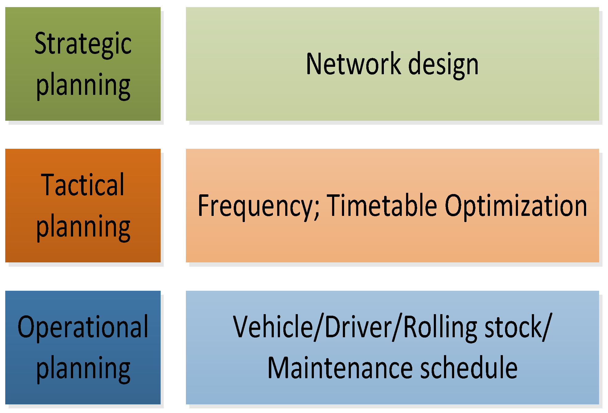
The urban rail transit system is processed from strategic planning, tactical planning and operational planning, as shown in Figure 1 [1,2,3,4]. Among tactical planning, line planning such as capacity, frequency and routing scheme should be considered, and timetabling including the planned arrival time and departure time of trains at each station should be considered. Numerous studies have proposed optimal models and algorithms for line planning [5,6,7,8] and timetabling [9,10,11,12] based on a single line and rarely considered the impact of passenger transfer for the whole network. In recent years, several subway operational companies have studied the overall optimization of metro network operation organization gradually to realize multiple operation indicators’ optimization through multidimensional decision making.
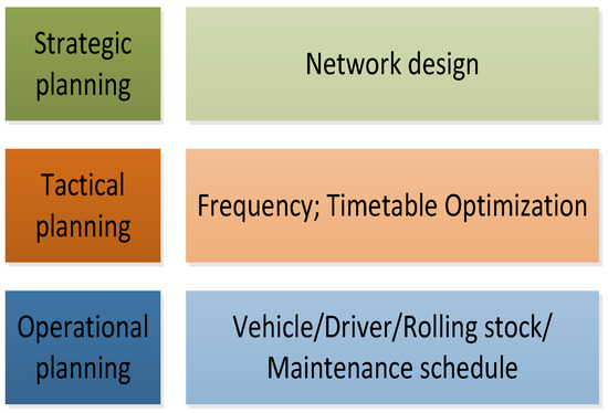
Figure 1.
Process and component of subway system.
Ref. [13] proposed a brand subway network operation organization optimization model based on the combination of cost and passenger satisfaction. The objective function considered the non-served passengers, fixed cost for full-length or short-turn trips with different capacity, and reward for transporting passengers. There are some problems such as unclear significance of the evaluation standard and difficulty in unifying the conversion. In addition, the optimization goal of minimizing stranded passengers by penalty factor in this model may make some stranded passengers stay at the platform all the time, which is inconsistent with the actual situation.
In this paper, an improved model based on the model in [13] is proposed, which also considers the operation cost and service quality. A passenger flow model based on queuing theory is adopted, which can better describe the passenger waiting time to solve the possible problem in Ref. [13]. In order to clarify the actual meaning of the objective function, the passenger satisfaction index is evaluated by multiplying the total passenger waiting time by the average wage per unit time of local personnel. By considering the operation cost and passenger waiting cost comprehensively, the social benefits of the subway network are evaluated from a unified perspective. At the same time, the subway system is often the preferred and fastest means of transportation in large cities for passengers, so passengers are restricted from waiting for no more than two trips to ensure that service quality.
Differing from Ref. [13], we linearize the nonlinear part of the optimization model, construct a subway line–network integrated optimization model and adopt the mixed integer quadratic programming algorithm, which has the advantages of accurate results and fast convergence, and can obtain a more accurate optimal solution than the heuristic method.
Combined with simulation cases, the proposed theoretical model is verified and analyzed, and compared with Ref. [13]. The results ratify the rationality and correctness of the model in this paper.
2. Passenger Flow Model Based on Queuing Theory
2.1. Subway Queuing System
Queuing theory is to solve the problem of optimal design and optimal control of corresponding queuing systems on the basis of studying the probability regularity of various queuing systems. A general queuing system has three components: input process, queuing and queuing rules, and service mechanism. For the subway queuing system, the main components are described as follows [14]:
- Passenger flow input process
The behavior of passengers arriving at the platform and waiting for boarding is a random process. Due to the small headway between two consecutive trips, the passenger flow changes little in a short time. If the passenger flow arrival rate of each station during operation is simplified to a fixed value, it is evenly distributed over time in each period. Its value can be obtained by analyzing the passenger flow arrival information of the urban rail transit automatic fare collection system (AFC) and calculating the average number of inbound passengers in this period.
- 2.
- System queuing and queuing rules
In the subway queuing system, passengers can queue up and receive services when they enter the system. The queuing rule is providing services according to the order of arrival of passengers, that is, who arrives earlier receives service earlier.
- 3.
- Service mechanism
The service mechanism of the queuing system includes the number of service desks, whether customers receive services individually or in batches, and the distribution of service time, among which the distribution of service time is more important. Due to the characteristics of double-track and single-direction operation of subway trains, the train provides one service at a time for a single service desk. The dwell time of a train can be abstracted as service time. The dwell time is generally a fixed constant, so it belongs to fixed length distribution. The train headway average can be abstracted as vacation time. Then, the subway train service process is a pure limited service vacation queuing model; that is, a single vacation system that enters the vacation state every time a service is provided.
2.2. Passenger Flow Model
The cumulative passenger flow on the platform is a random variable that changes with time. Not only passengers on the line need to be considered, but also passengers transferred from other lines. Therefore, the cumulative passenger flow on the platform is mainly composed of two parts: the internal passenger flow transferred by other lines and the passenger flow from other external transportation connected to the urban rail system. Based on the analysis of the composition of the subway system with queuing theory, the external passenger at each station is set to be evenly distributed. We assume that passengers arrive at the station evenly with arrival rate , and then the external passenger flow arriving at the platform in unit time is , as shown in the shadow area in Figure 2. There is a linear correlation between the number of passengers at the platform and headway between two consecutive trips.
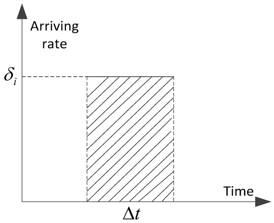
Figure 2.
External passenger at the platform in unit time.
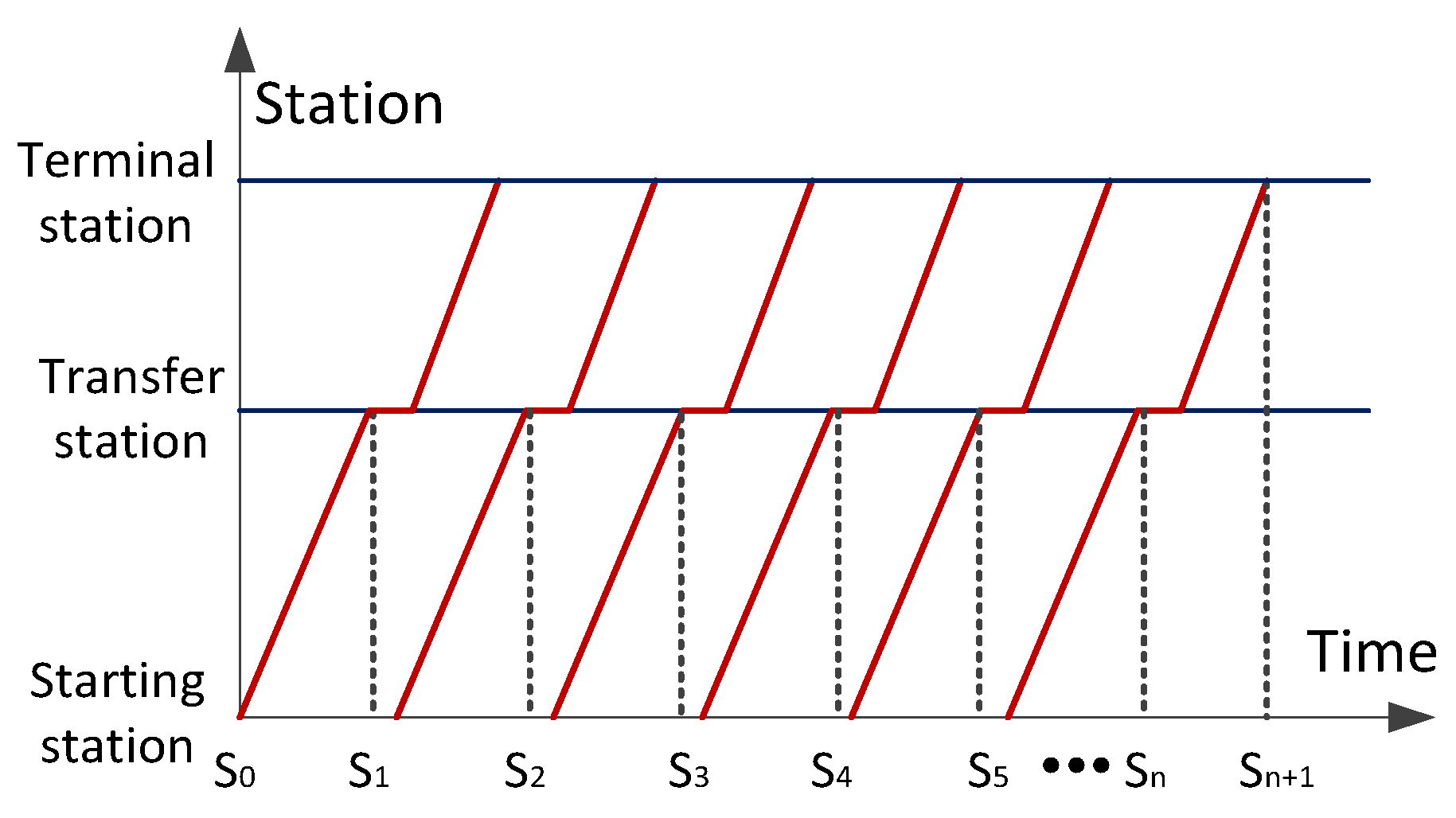
As for passenger flow at the interchange station, a transfer proportion parameter is assumed, which means that passenger flow transported from the front stations transfers to other lines based on the transfer proportion. Short turning strategy is also considered in this model, and passenger flow for full-length trips and short-turning trips are different; therefore, the transfer passenger flow can be calculated according to whether the line operates short turning strategy. However, the passenger flow from the front stations is different in different periods, so the passenger flow calculation at the interchange station needs to be a variable that depends on the arrival times of each trip at the interchange station, as shown in Figure 3. We divide the time into segments (S0, S1, …, Sn+1) and the 0–1 variable is introduced to describe which segment belongs to a trip’s arriving time.
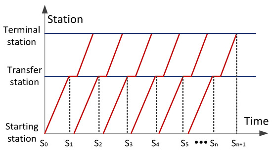
Figure 3.
Time division diagram of internal passenger flow.
3. Optimization Model of Subway Operation Cost and Passenger Satisfaction
3.1. Objective Function and Definition
The optimization model of subway network timetabling based on passenger flow established in this paper mainly considers two performance indexes: operation cost and service quality. In order to reflect the above performance indicators, a multi-objective optimization function is constructed, which includes three contents: first, the fixed cost required for trains with different capacities on different lines to operate full-length trips and short-turn trips; second, the ticket price profit obtained by transporting passengers on different lines with different routing schemes; third, the passenger waiting time. The former two objective functions are used to evaluate the operation cost, and the latter is used to evaluate the service quality. The specific description of the objective function is as follows.
3.1.1. Operating Cost Assessment
In this paper, we comprehensively evaluate the operating cost performance index according to the fixed cost based on train capacity, routing scheme and the profit of transporting passengers.
For different lines, the cost is different for operating a full-length trip or short-turn trip with different capacities, which can be obtained based on the operation history data. It is a fixed parameter value, which is only related to the selection of train capacity scheme and routing scheme. Once it is selected, the cost is determined. The specific calculation formula of this part is as follows:
where represents the line index in a subway network and represents a set of lines in the network. According to whether the line can operate short-turn trips, the line set is divided into two subsets, namely (line set without short-turns) and (line set enabling short-turns trips). represents a set of the train trips on the line , is the train trip index, represents a set of the train capacities, and represents the selected train capacity. and respectively represent the fixed cost value of a full-length trip and a short-turn trip on the line with train capacity . and are 0–1 variables. The value of equals 1 only if the trip with capacity is a full-length trip on line , and the value of equals 1 only if the trip with capacity passes through each station in the short-turn area on the line. It should be noted that when the value of equals 1, the trip may be a short-turn trip or a full-length trip, because the full-length trip will also pass through the short-turn area. Therefore, whether a trip is a full-length one or a short-turn one needs to be determined in combination with the values of the two variables, and . It can be seen that some trips cannot exist in reality when and are combined. For example, when = 1 but = 0, the trip covers all stations of one line of LS but does not traverse the short-turn stations. Or, when = 0 and = 0, the trip does not traverses any stations of one line of LS. The trips that cannot exist in practice are defined as “fake trips”. So, there are the following possible situations:
- (a)
- and , if trip is a full-length trip.
- (b)
- and , if trip is fake trip that does not exist.
- (c)
- and , if trip is a short-turn trip.
- (d)
- and , if trip is fake trip that does not exist.
On the other hand, based on the OD (origin to destination) passenger flow in the urban rail transit network, the passenger flow transmitted by different lines in the network can be counted to obtain the total income of transporting passengers, as shown in the following formula:
where represents the set of stations on the line and is the site index. represents the unit revenue of transporting a passenger from the station to the station on the line . and refer to the passengers transported by full-length and short-turn trips, respectively. If the line cannot operate a short-turn trip, indicates the total number of passengers who get on the train from the station before to the station of a full-length trip on the line . If the line can operate a short-turn trip, it is necessary to calculate the number of passengers transported by the full-length trip trains , the number of passengers transported by the short-turn trip trains , and the number of passengers whose destination is out of the short-turn area but take a short-turn trip to the short-turn terminal station and transfer to the full-length trip .
3.1.2. Service Quality Assessment
Based on the performance index of urban rail network service quality, our work aims to reduce the waiting time of passengers in the network. Based on queuing theory, the waiting time of passengers can be calculated as:
According to the hourly wage standard of 24 yuan/h in Beijing, the waiting time of passengers is converted into wage cost as follows:
In the formula, it is assumed that the passengers at each platform arrive at the station evenly according to a certain arrival rate, and the waiting time of passengers is closely related to the headway of departure times.
3.1.3. Comprehensive Performance Evaluation
For the comprehensive performance of the urban rail network operation organization, the two performances of operation cost and service quality need to be considered. Based on the calculation of the above two performance indexes, the optimal objective function can be calculated as:
Since the orders of magnitude and dimensions of the three objective functions are different, the min–max range standardization method is used to normalize the multi-objective optimization function:
So, the normalized objective function is:
After normalization, the multi-objective optimization function can realize the comparative analysis under the same dimension.
3.2. Constraints Description
3.2.1. Train Trips Constraints
Group C1 constraints restrict the full-length trips, short-turn trips and fake trips of each line in the network according to whether the line can operate the full-length trips and short-turn trips. For example, the first and last train trips of the line are limited to be true. If the trip on the line is a full-length trip, the values of and both equal 1. If the trip on the line is a short-turn trip, then equals 0 and equals 1.
3.2.2. Time Constraints
This set of constraints mainly limits the arrival and departure times of each trip on the line at different stations.
Group C2 constraints limit the departure time of the first train and the last train at the starting station to the time domain boundary value of train timetable. In addition, for the trips on the line , the departure time of two adjacent trains at the same station shall be limited to meet a certain safety interval IS and not exceed the maximum planned time for the full-length trips and short-turn trips.
In this set of constraints, the last formula is the constraint on the waiting time of passengers. The left side of the inequality is the waiting time of passengers, and the right side is the product of two departure intervals and the number of passengers stranded at the current platform . This formula limits the waiting time of passengers arriving at the platform evenly to no more than two departure intervals, which means that the stranded passengers who fail to catch the first train must get on the second train.
3.2.3. Passenger Flow Constraints
This group of constraints mainly ensures that the number of passengers transported by a full-length trip or a short-turn one on all lines does not exceed the train capacity.
The first two constraints of the group C3 limit the passenger capacity of enabling and not enabling the short-turn trips line according to the line attributes to not exceed the train capacity . The last four constraints also limit the number of passengers transported by the train not to exceed the accumulated passenger flow at the platform for different line attributes, including passengers waiting at the station and stranded passengers. represents the cumulative passenger flow from time 0 to time , and its value includes internal passenger flow and external passenger flow. Among them, the external passenger flow enters the station evenly at a certain arrival rate according to the above queuing theory. The internal passenger flow is transferred according to a certain proportion of the passenger flow to the transfer station based on the OD data.
3.2.4. Stranded Passenger Variable of True Trips
Group C4 constraints are used to calculate the number of stranded passengers of true trips, i.e., . is a large enough integer. At the same time, in order to meet the actual operation of the subway and avoid the situation that there are still passengers stranded in the system after the end of operation, the passenger retention of the last train number of each line at each station is limited to 0; that is, all passengers must be completely transported in the last train.
3.2.5. Internal Passengers Flow
The cumulative passenger flow can be calculated by the sum of external passenger flow and internal passenger flow . As mentioned above, the passenger flow calculation at the transfer station depends on the arrival time of trips at the transfer station. Therefore, for passengers who want to transfer from line to line at transfer station , the arrival times can be calculated by Equation (13).
where is the dwell time for trip at transfer station on line . Then, the time span is divided into several segments with =0, =T. The passengers who would like to transfer from line to line at the transfer station can be calculated as follows:
Then, the following constraints should be considered in this model.
The first constraint of C5 calculates the number of internal passengers until the time instant . is a 0–1 variable that equals 1 when the time instant is larger than the break-point and smaller than , and equals 0 in other conditions as described in the second constraint. The third one ensures that only one of these time segments is identified for each time instant .
In addition to the above five sets of constraints, the model also limits the boundary values of each decision variable of the train, such as the departure time of each line train at each station is within the time domain of train diagram planning, the passenger capacity is positive and the number of stranded passengers is positive.
4. Optimization Algorithm
Combined with the above constraints and objective function, the final optimization model is as follows:
There are several nonlinear items in the former two constrains of C5, such as the product of a binary variable and a real-valued variable. Therefore, we introduce a property to linearize this nonlinear item.
For example, considering the product of a binary variable and a real-valued variable , we introduce a new auxiliary real-valued variable to replace the product ; then, the following constraints should be satisfied:
The nonlinear items and also are equivalent to new real-valued variables with corresponding constraints.
The model established by the above problem is a mixed integer quadratic programming model (MIQP); that is, a mixed integer programming problem with a quadratic objective function but no quadratic constraint, which can be solved in combination with IBM ILOG CPLEX.
A mixed integer nonlinear programming model is constructed in Ref. [13] and solved by the divide and conquer heuristic algorithm, taking one line as the initial line and the optimization result as the input of the next line, and then iterating to the maximum number of iterations. In contrast, the mixed integer quadratic programming model constructed in this paper can be solved directly by solver to obtain the global optimal solution. In addition to the quality of understanding, the computational efficiency has been greatly improved in the simulation verification cases.
5. Simulation Analysis and Verification
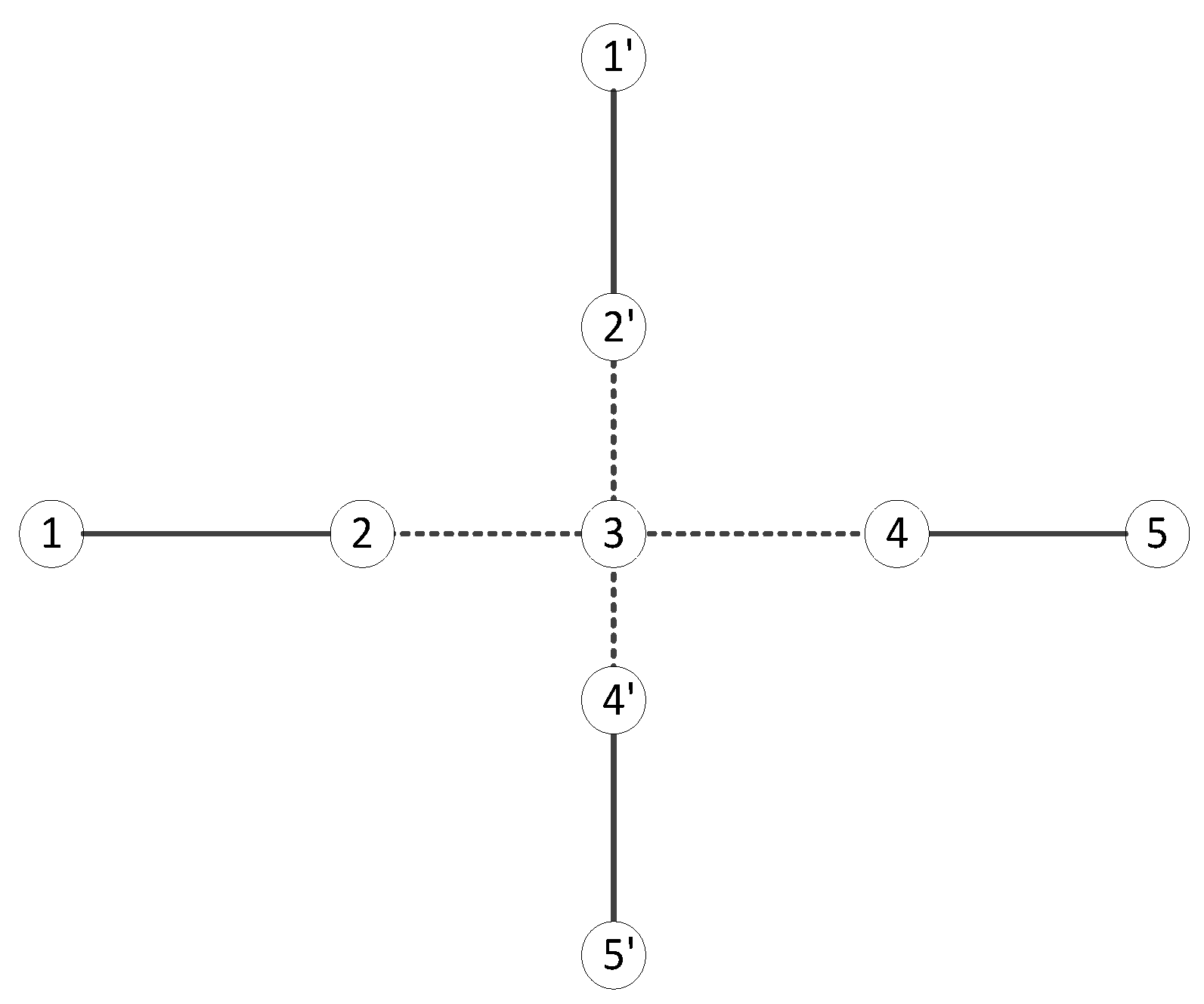
To assess the performance of the proposed model and algorithm, we designed a case study with two physical lines which are the same as Ref. [13]. Some parameters of the simulation model in this paper, such as line transfer rate and OD passenger flow, are also consistent with Ref. [13]. The layout is shown in Figure 4. The following case study was performed on a computer with an InterR Xeon Gold6136@3.00Ghz processor and 6.00 GB RAM.
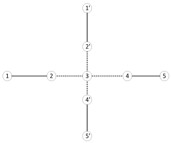
Figure 4.
Layout of subway lines.
There are five stations for each line, and all can operate short-turn trips. The short-turn area is shown as dotted lines. Station 3 is an interchange station for both lines. According to the definition of lines in this model, which is different from the physical line, there are four lines that need be scheduled, because line 1 and line 2 are the same physical line with the same number of stations but opposite directions, the same is true for line 3 and line 4.
The time span is 20 min, and the maximum trip number is eight for each line. The minimum safety headway is 2 min. To compare with [13], we keep the same assumption that all the passengers in the subway system insist on staying and waiting. Two possible capacities of trains can be chosen, . The fixed cost for operating a full-length trip with a capacity of 800 and 1600 is 42 and 84 yuan, respectively. The fixed cost for operating a short-turn trip with a capacity of 800 and 1600 is 22 and 28 yuan, respectively.
The OD and rewards per passenger matrices for line 1 and line 2 are shown in Table 1 and Table 2. The top right-hand corner contains data for line 1, and the bottom left contains data for line 2. The transfer ratio is set to be 0.4 at each transfer station for all lines to be consistent with [13].

Table 1.
OD matrix for line 1 and line 2.

Table 2.
Rewards per passenger for line 1 and line 2.
We set the same external passengers as Ref. [13] for each line, as shown in Table 3. There are 50, 100, 120, 90 and 0 people per min coming into the subway system from station 1 to station 5, respectively.

Table 3.
External passengers per minute for each line.
According to the parameters above, the optimal results can be obtained by CPLEX. For example, the optimal train schedule and passenger flow variation for line 1 are shown in Table 4. The loads of all trips except the first one reach the train capacity, which means a high transportation efficiency. The average waiting time for excess passengers in line 1 is about 2 min because they get on the next train if they are stranded. Finally, there are no passengers stranded as the load for each trip at station 5 is zero, which means that all passengers are transported to their destinations. Six true trips are operated during this period with an average headway of 200 s.

Table 4.
Optimal train schedule and passenger variation for line 1.
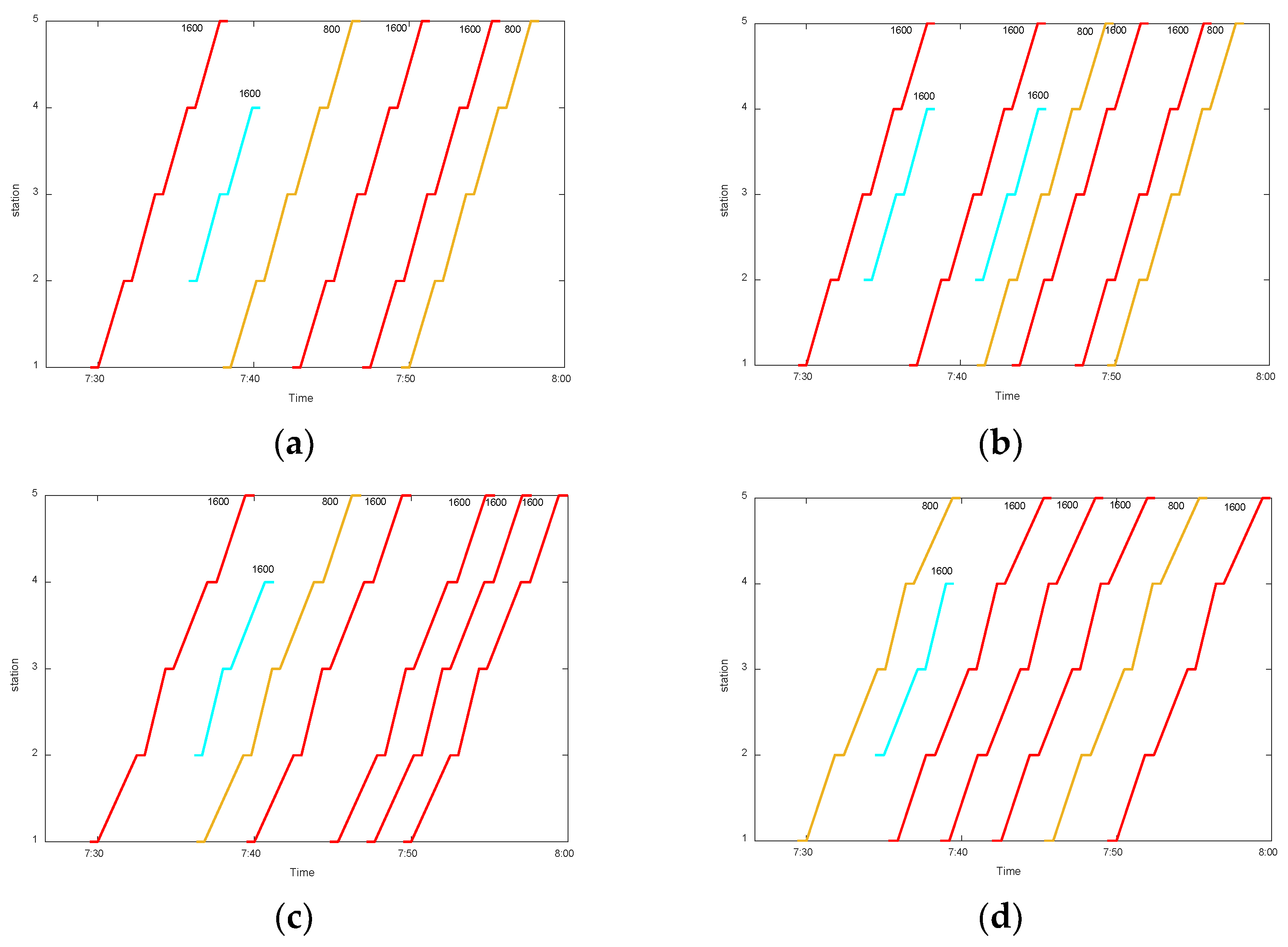
Figure 5 depicts the train diagrams for all lines. Different lines have different numbers of true trips, short turning strategies and capacities because of the different passenger demands for each line. Comparing the train diagrams for line 1 and line 2, there are two more true trips for line 2 as the number of external passengers is larger, especially for station 2.
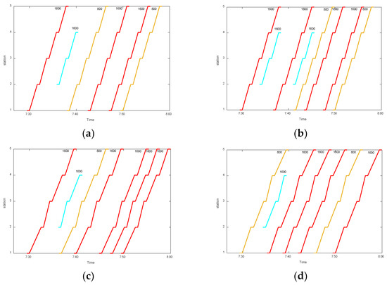
Figure 5.
Train diagrams for all lines with different short turning strategies and train capacity choices. (a) train diagram for line 1; (b) train diagram for line2; (c) train diagram for line 3; (d) train diagram for line 4.
For normalization, the maximum and minimum values for each objective function can be estimated roughly by the size of the case study. Based on normalization, objective function values for each dimension can be obtained to assess the model performance, which are shown in Table 5. The objective function “Cap” plays a more important role in the three parts of objective functions, followed by “Reward”, which is closely related to the ticket prices implied in Table 2.

Table 5.
Objective value for each function.
The calculation time is 15.4 min and the gap ((Upper Bound-Lower Bound)/Upper Bound) is 5.23%. The performance for calculation has been improved significantly compared with [13].
6. Conclusions and Future Work
In this paper, we established a subway line–network integrated optimization model for line planning and timetabling based on passenger flow. The operation cost and service quality are taken as the optimization goals. The service quality is evaluated by passengers’ waiting cost, calculated by multiplying the total passenger waiting time by the average wage per unit time of local personnel. Thus, operation cost and service quality index can be added directly. A passenger flow model based on queuing theory is used to describe the relationship between passenger flow change and passenger waiting time. Furthermore, the objective function is normalized to realize the comparative analysis under the same dimension. By linearizing the nonlinear item in the optimization model, the mixed integer quadratic programming model is adopted for the solution. At last, a sample two-line network model, including an internal and external passenger flow module, schedule module, etc., is simulated and analyzed, which validated the proposed optimization model. In the network, we consider the passenger transfer activities, train capacity scheme and routing scheme.
However, we constructed the passenger flow model and cost model with various assumptions and simplifications, without considering the influence of passenger flow heterogeneity and randomness, as well as train operation strategy, which may be different from the actual situation, and should thus be refined. The simulation verification case in this paper is relatively simple, and most of the input data used are not from the actual line. In the next step, we need to carry out further application research according to the more complex line network operation conditions in combination with the actual line. In addition, the development of simulation tools for the optimal operation of subway networks must also be carried out simultaneously.
Author Contributions
Conceptualization, W.M.; methodology, Y.Z. and Z.Z.; software, M.Z.; validation, G.Q. and M.Z.; formal analysis, G.Q.; investigation, G.Q.; resources, M.Z.; data curation, M.Z.; writing—original draft preparation, Y.Z. and M.Z.; writing—review and editing, Y.Z.; visualization, Y.Z.; supervision, W.M.; project administration, W.M.; funding acquisition, W.M. All authors have read and agreed to the published version of the manuscript.
Funding
This research was funded by Hunan Young Talent Project, grant number 2018RS3137.
Institutional Review Board Statement
Not applicable.
Informed Consent Statement
Not applicable.
Data Availability Statement
Not applicable.
Conflicts of Interest
The authors declare no conflict of interest.
References
- Lu, K.; Han, B.; Zhou, X. Smart Urban Transit Systems: From Integrated Framework to Interdisciplinary Perspective. Urban Rail Transit 2018, 4, 49–67. [Google Scholar] [CrossRef]
- Desaulniers, G.; Hickman, M. Handbooks in Operation Research and Management Science; Public Transit: Tokyo, Japan, 2007; Volume 14, pp. 69–128. [Google Scholar]
- Ibarra-Rojas, O.J.; Delgado, F.; Giesen, R.; Munoz, J.C. Planning, Operation, And Control of Bus Transportation Systems: A Liter-ature Review. Transp. Res. Part B Methodol. 2015, 77, 38–75. [Google Scholar] [CrossRef]
- Wang, Y.; D’Ariano, A.; Yin, J.; Meng, L.; Tang, T.; Ning, B. Passenger demand oriented train scheduling and rolling stock circulation planning for an urban rail transit line. Transp. Res. Part B Methodol. 2018, 118, 193–227. [Google Scholar] [CrossRef]
- Ozuysal, M.; Sengoz, B. Capacity Based Operation Planning of Rail Transit Systems: A Case Study for Izmir Light Rail Transit. In Proceedings of the World Conference on Transport Research, Istanbul, Turkey, 4–8 July 2004. [Google Scholar]
- Yan, F.; Goverde, R.M. Combined line planning and train timetabling for strongly heterogeneous railway lines with direct connections. Transp. Res. Part B Methodol. 2019, 127, 20–46. [Google Scholar] [CrossRef]
- Shafia, M.A.; Sadjadi, S.J.; Jamili, A. Robust Train Formation Planning. Proc. Inst. Mech. Eng. Part F J. Rail Rapid Transit 2010, 224, 75–90. [Google Scholar] [CrossRef]
- Zhang, M.; Wang, Y.; Su, S.; Tang, T.; Ning, B. A Short Turning Strategy for Train Scheduling Optimization in an Urban Rail Transit Line: The Case of Beijing Subway Line 5. J. Adv. Transp. 2018, 2018, 1–19. [Google Scholar] [CrossRef]
- Zhou, X.; Ming, Z. Single-track Train Timetabling with guaranteed optimality: Branch-and-bound Algorithms with enhanced lower bounds. Transp. Res. Part B Methodol. 2007, 41, 320–341. [Google Scholar] [CrossRef]
- Xu, X.; Li, K.; Yang, L.; Ye, J. Balanced Train Timetabling on A Single-line Rail Way with Optimized Velocity. Appl. Math. Model. 2014, 38, 894–909. [Google Scholar] [CrossRef]
- Shafia, M.A.; Aghaee, M.P.; Sadjadi, S.J.; Jamili, A. Robust Train Timetabling Problem: Mathematical Model and Branch and Bound Algorithm. IEEE Trans. Intell. Transp. Syst. 2012, 13, 301–317. [Google Scholar] [CrossRef]
- Liu, P.; Han, B. Optimizing the train timetable with consideration of different kinds of headway time. J. Algorithms Comput. Technol. 2017, 11, 148–162. [Google Scholar] [CrossRef] [Green Version]
- Blanco, V.; Conde, E.; Hinojosa, Y.; Puerto, J. An optimization model for line planning and timetabling in automated urban metro subway networks. A case study. Omega 2019, 92, 102165. [Google Scholar] [CrossRef]
- Ning, Z. Study on Optimization Algorithm of Urban Rail Transit Train Operation Adjustment Considering Passenger Flow Change. Master’s Thesis, Lanzhou Jiaotong University, Lanzhou, China, 2019. [Google Scholar]
Publisher’s Note: MDPI stays neutral with regard to jurisdictional claims in published maps and institutional affiliations. |
© 2022 by the authors. Licensee MDPI, Basel, Switzerland. This article is an open access article distributed under the terms and conditions of the Creative Commons Attribution (CC BY) license (https://creativecommons.org/licenses/by/4.0/).

