1. Introduction
Increasing the efficiency of vehicle drive systems is one of the highest goals in the automotive industry. By reducing energy consumption, further benefits such as an increase in electric range or reduced vehicle mass can be realized. Since drive systems are occasionally oversized in terms of performance for the actual requirements, efficiency can be increased by adjusting the performance [
1,
2,
3,
4]. This increase in efficiency can be achieved by reducing the performance of a drive system to the requirements that customers mostly need in daily operation. Furthermore, a second drive system is required in order to enable high demands, which occur rather rarely.
As part of a dissertation, this publication gives an insight into the method for analyzing customer-relevant driving requirements and converting them into relevant target values for the design of overall drive systems. In the context of the dissertation, an overall drive system is designed which combines increased efficiency by focusing on the core area of customer needs with high functionality by covering high requirements.
2. Methods
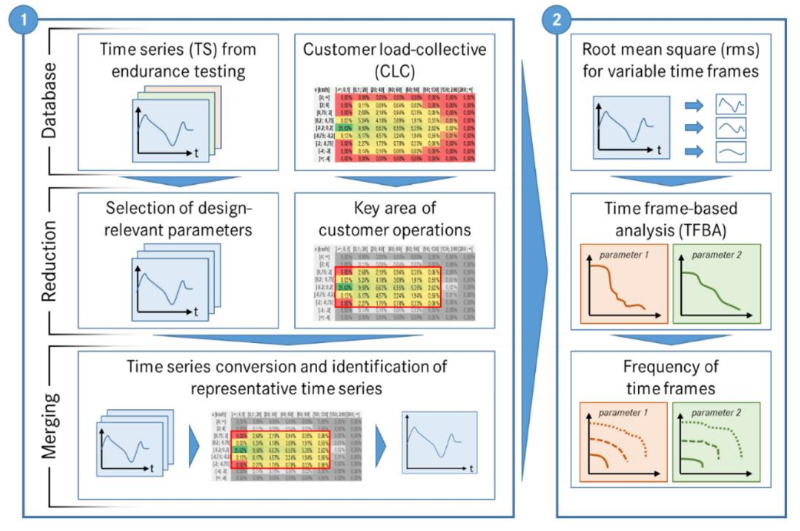
This paper is divided into two methodical approaches as shown in
Figure 1: first, time series data (TS) from endurance testing are compared with statistical customer data (CLC) with regard to identifying customer-relevant time series. In the second step, the root mean square (rms) is calculated for different widths of time frames and the time frame-based analysis (TFBA) is used to derive design-relevant parameters for the overall system design.
2.1. Database
The first approach is based on two types of data, namely time series and customer load collective. The available time series data are records of various signals from endurance testing, from which the relevant load variables that are required for the drive system design must be selected. The main design-relevant parameters are the mechanical power and the torque on the wheel. In addition, the vehicle speed, respectively the wheel speed as well as the acceleration, is also used to identify representative time series. Dependent on the available customer data, other parameters may be considered.
The available customer data are the results of event-based counts in the control unit of the customer vehicles, so-called
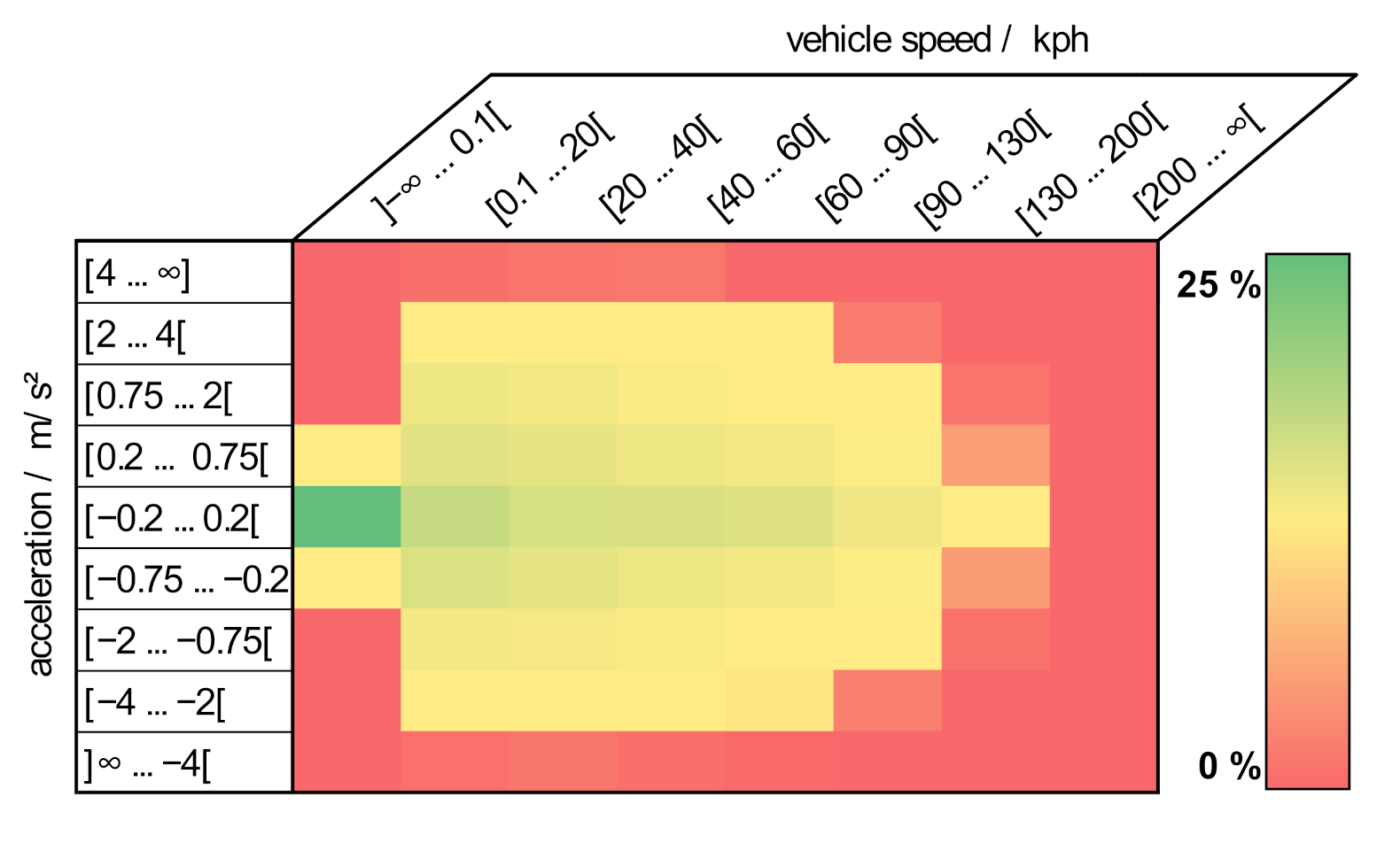
customer load collective. These counts provide information about the frequency distribution, i.e., how often certain events occur. They are shown in
Figure 2 using the example of the vehicle speed and acceleration distribution while the drive system is active. The color scheme represents the accumulation of the customer’s driving behavior. According to the color bar, the vehicles in customer operation actually do not drive at all about 25% of the time despite the ignition being switched on.
The largest accumulation in these statistical distribution matrices of around 95% covers the range between approximately 0 and 130 kph as well as −2 and 2 m/s
2. This conspicuity is also reflected in [
5], where the driver behavior of the 34 participants is analyzed based on recorded real drives over a distance of around 35,000 km. The evaluation shows that the highest accelerations actually driven in the speed range up to approximately 100 kph are below 1.5 m/s
2 and at speeds of up to 140 kph are mostly not higher than approximately 1.0 m/s
2. The limitation of the speed range to a maximum of 130 kph is derived from [
6]. According to this report, the average top speed on German highways without speed limit is between 110 and 130 kph. Abroad, this value is lower due to speed limits. Based on these findings, accelerations between −2 and 2 m/s
2 and speeds of up to 130 kph can initially be assumed to be customer relevant. Consequently, this area can be identified as the focus of customer driving operations and used as the basis for a customer-specific drive system design.
2.2. Comparison of the Data Bases and Derivation of Representative Time Series
After selecting appropriate, design-relevant signals from the time series data and determining the focus of customer driving operations, the next step is to merge these two databases. For this purpose, distribution matrices for all time series are created analogous to the customer data. The aim is to describe the time series statistically by transferring them into heat maps such as acceleration versus vehicle speed, as shown above in
Figure 2, as well as motor torque versus motor speed with the same clustering as the CLC data.
The deviation of these matrices from the CLC data is the measure of the customer relevance of the time series. First, the cell-specific deviation |
Xi,j| as absolute value of the cell-by-cell difference between time series
cellTS and
CLC data
cellCLC is calculated according to Equation (1).
The relevance of each time series is evaluated based on the mean total deviation. In this respect, the time series, whose deviation is the smallest, represents the best approximation to the customer distribution matrices. As shown in Equation (2), the arithmetic mean of the total deviation
is the sum of all cell-specific deviation values |
Xi,j| divided by the number of all cells
n in the above-mentioned area of greatest customer operation.
This approach allows the time series to be sorted in ascending order by their total mean deviation. According to the method of [
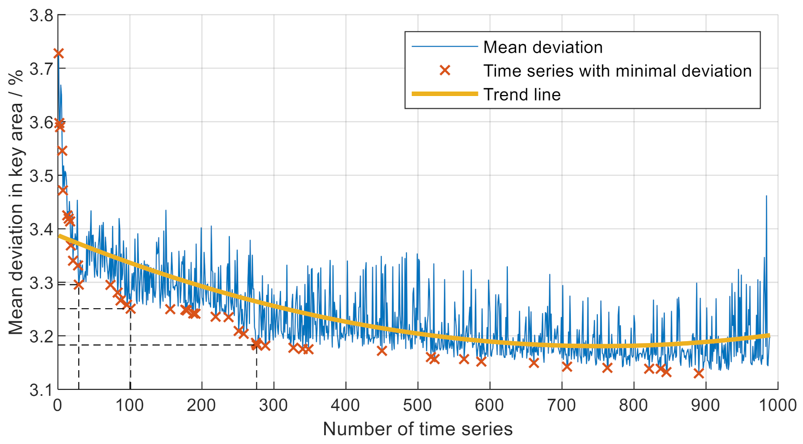
7], time series are combined with one another to minimize the total deviation, starting with those two, whose deviation is the lowest. Increasing the number of combined time series leads to a decrease in the mean deviation, as shown by the blue curve as well as the yellow trend line in
Figure 3. The red markers highlight exactly that time series whose combination leads to the smallest deviation of the key area pointed out in
Section 2.1.
In this case, 1000 time series are evaluated, of which the combination of all 45 red-marked time series shows minimal total deviation. In other words, combining exactly these 45 out of the 1000 time series, which the markers indicate, reduces the deviation the most and leads to the minimum of 3.13 in mean deviation.
Following the steep drop, the slope decreases with an increasing number of time series and the mean deviation decreases only slightly. Due to the trade-off of reducing the mean deviation as much as possible while at the same time minimizing the computational effort, the red regression curve shows several optima displayed by the dashed black lines. According to these, considering 12 specific time series, indicated by the first 12 markers from the left, would lead to the first big decrease in the mean deviation from about 3.7 to 3.3. The second and third dashed lines show the consideration of 17 and 28 time series, respectively, with a decrease in the mean deviation to 3.25 as well as 3.18, respectively. In this respect, considering these numbers of time series represents optimums regarding computational effort and deviation in order to describe customer behavior in the best possible way.
2.3. Validation of the Purposed Method
This methodological approach must take into account that the derivation of certain time series from statistics such as CLC data is ambiguous due to the lack of the time reference. In this case, the statistical frequency distribution can only be approximated by selecting suitable time series. In contrast, the reverse method of statistical representation of a time series represents a clear correlation.
Despite the lack of unambiguity, the procedure is admissible, as this method aims to approximate, rather than exactly represent, customer requirements by combining several time series.
In order to ensure the plausibility of the method, a given time series is first transferred into a distribution statistic for unambiguous assignment. In the next step, the method from [
7] is used to analyze imported time series, one of which is the given one, with the aim of deriving the initial time series. The result of this analysis was a calculated deviation of zero. This shows that the procedure is able to re-identify the originally read-in time series, thus proving its functionality. To further check the plausibility, this process is repeated twice on top of that. Both different as well as the same time series are combined several times with one another and the method is applied, leading to the same result both times.
In addition, the available customer data represent a solid database due to the extensive amount of data. Using the example of an investigated model series, the data contains more than 15,000 vehicles with a total mileage of more than 100 million km. These selected vehicles all have a certain minimum mileage to evaluate only representative customer driving profiles. Reverse driving is also taken into account. This signifies a meaningful statistic, both in terms of different customer types and markets.
Furthermore, as already pointed out in
Section 2.1, the entire heat map of customer data is not of equal interest, but rather the focus of the research is on the area of greatest accumulation.
2.4. Time Frame-Based Analysis (TFBA)
The second methodological aspect introduces the time frame-based analysis according to [
8]. This method is used to identify design-relevant loads based on time-dependent criteria and to further evaluate their intensities, durations and frequencies, which is necessary for the design of drive system components.
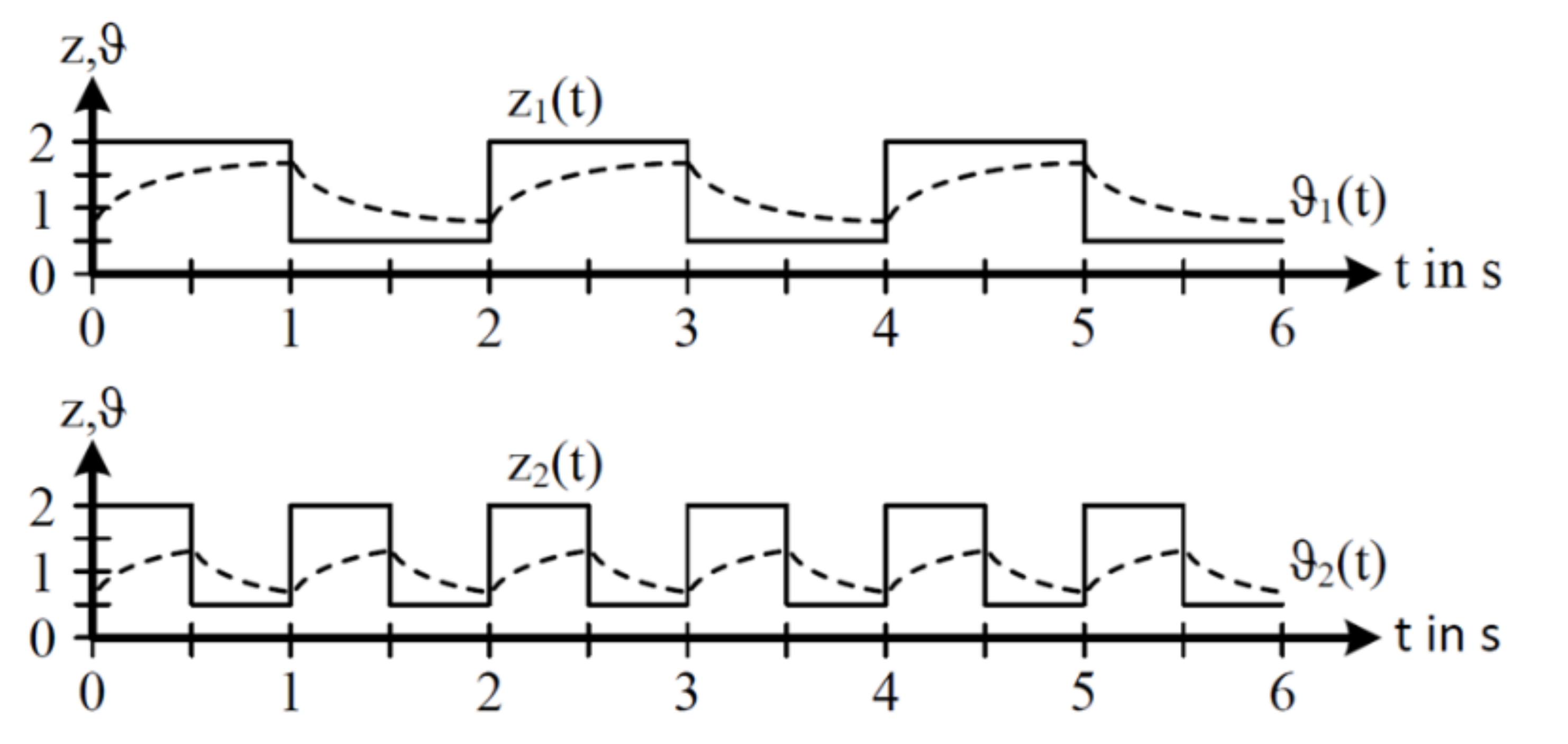
For illustration,
Figure 4 schematically shows two loads, z
1 and z
2, which are identical with respect to their classic statistical properties such as the root mean square (rms) z
rms, the minimum value z
min and maximum value z
max as well as their distribution functions.
Since these parameters do not provide any time-related information such as duration and frequency or the time interval between specific loads, the characteristics of these two loads cannot be compared. This circumstance is illustrated by the different temperature curves 𝛝1 and 𝛝2, which leads to different temperature gradients and thus, different thermal stresses on the components.
Therefore, the time frame-based load analysis is needed, in which time frames
τtf with continuously increasing width are defined and shifted over the time series [
9]. According to Equation (3), the maximum rms value is calculated for each time frame width.
For this purpose, the conditions pointed out in Equation (4) need to be considered: The time frame width
τtf must be at least equal to the time step width Δ
t. Additionally, the overall time series length
T must be extended to length
ttotal to ensure considering sufficient values for the largest time frame
τtf,max at the last time step
t =
T. Finally, the time frame is moved over the whole time series from
t = 0 to
t =
T.
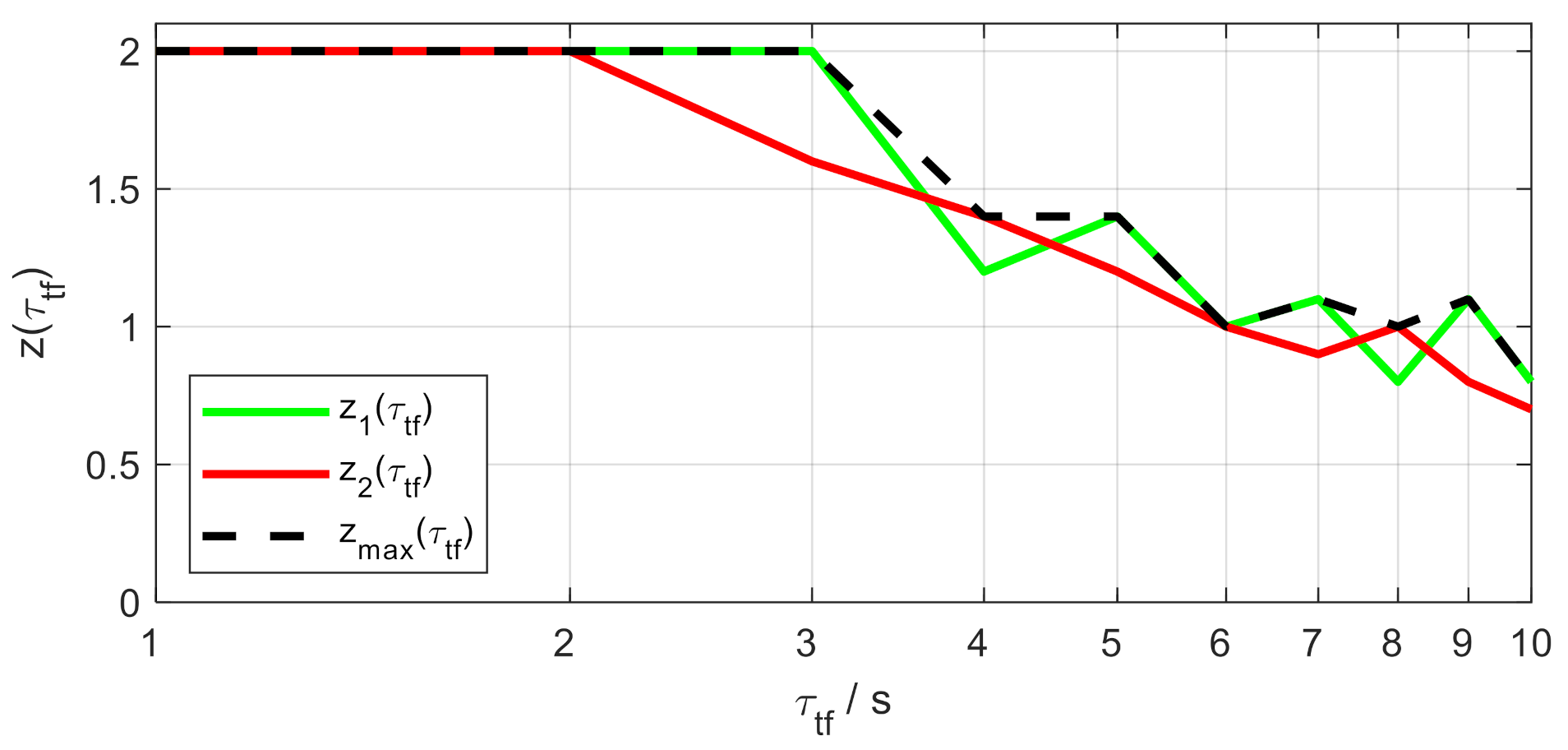
Figure 5 shows the resulting time-related continuous load curves for the two loads mentioned above. The diagram displays the maximum values for both loads z
1 and z
2 and each time frame width, which indicates that the respective rms value is demanded at least once for that frame.
As expected from the temperature curves 𝛝1 and 𝛝2 above, the comparison between the two signals at τtf = 3 s indicates that the rms value z1 is greater than z2. This leads to the envelope curve zmax, which represents the overall highest value of all loads. These highest values indicate maximum thermal load and are therefore crucial for the system design.
This method allows the analysis of different time series, regardless of their length. However, only those physical quantities that are directly proportional to the losses of a component can be analyzed [
9]. With respect to the design of drive systems, power and torque are suitable quantities.
2.5. Frequency of Time Frames
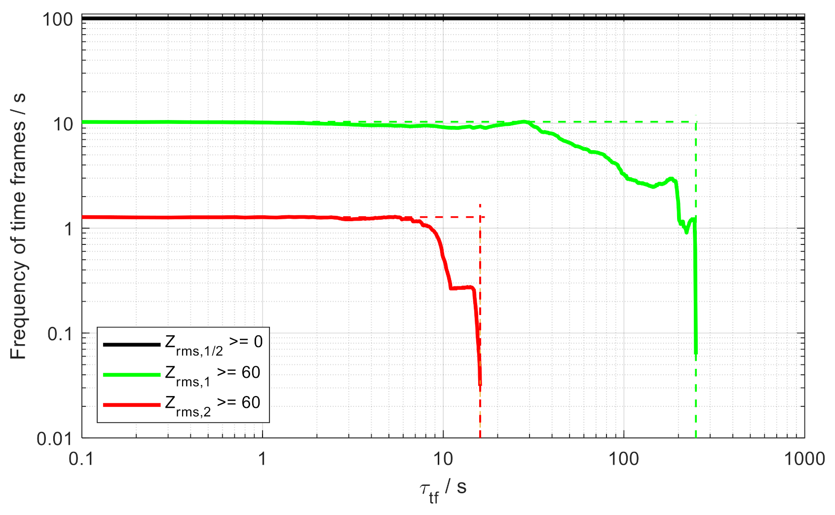
Finally, the analysis of the frequency of time frames evaluates the correlation of duration and frequency of occurrence. By displaying the time frame frequency over the time frame width, as shown in
Figure 6, different loads can be compared by evaluating how often and for how long certain loads occur.
The curves visualize the duration and frequency of the rms value of both loads z1 and z2. First of all, the black graph shows that all rms values are positive for both loads, so, as expected, the frequency of the rms value is 100%. Additionally, the figure displays the curves for an exemplary threshold value of 60, so the curves show the rms values zrms ≥ 60. In this case, zrms,1 is greater than zrms,2, both in terms of duration and frequency. This not only means that the time frame τtf,1 for this specific rms value is longer, but also the frequency of occurrence in this load has a higher share in the overall process. This leads to z1 being critical for the system design. With the help of these analyses, loads of different duration, intensity and characteristics can be compared and design-critical loads can be identified.
3. Conclusions and Future Work
The method introduced in this work allows the derivation of relevant parameters for the design of vehicle drive systems based on statistical customer data. For this purpose, time series are analyzed by comparing them with customer data. The aim is to identify customer-representative time series. Furthermore, these representative time series are investigated using the time frame-based load analysis. This procedure of describing the time-dependent characteristics of a time series allows the detection of design-critical loads and generates relevant parameters for the system design.
These relevant parameters such as peak values and continuance values for torque and power as well as working points and sweet spots represents the input for the design of overall drive systems. By limiting this input to the most frequently required customer needs, the efficiency of the overall system can be increased.


