
A Development of a New Image Analysis Technique for Detecting the Flame Front Evolution in Spark Ignition Engine under Lean Condition


Abstract
:1. Introduction
2. Experimental Setup
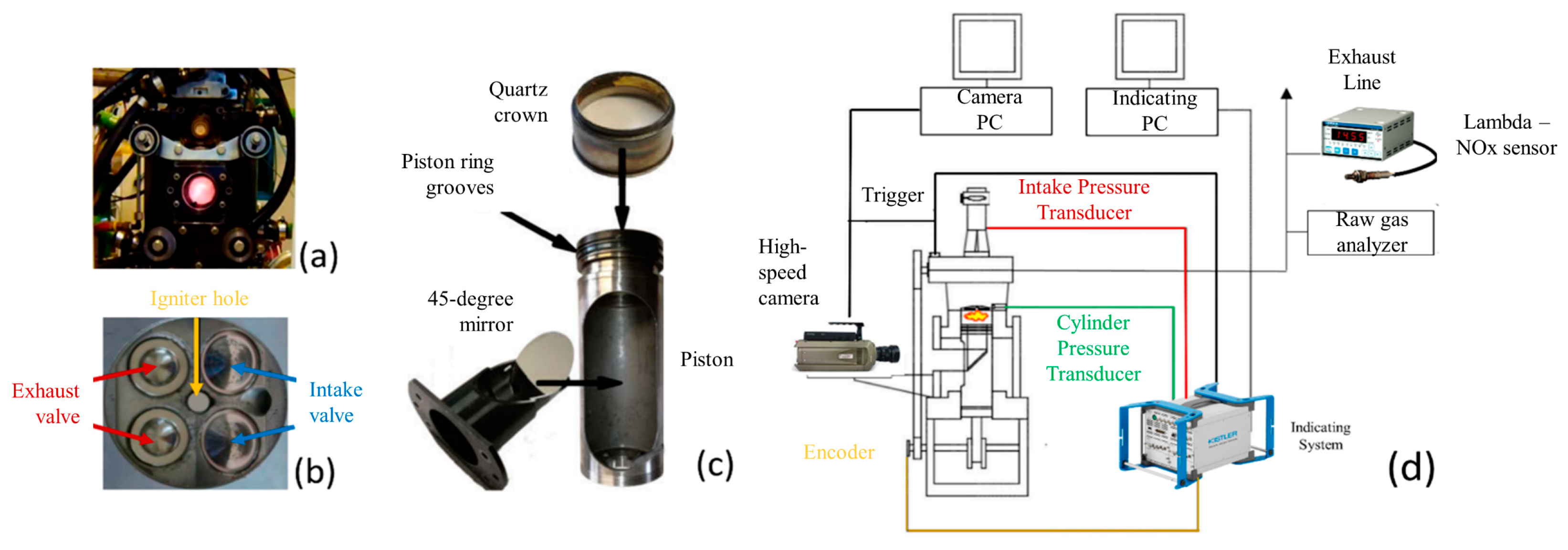
2.1. Optical Access Engine
2.2. Imaging System
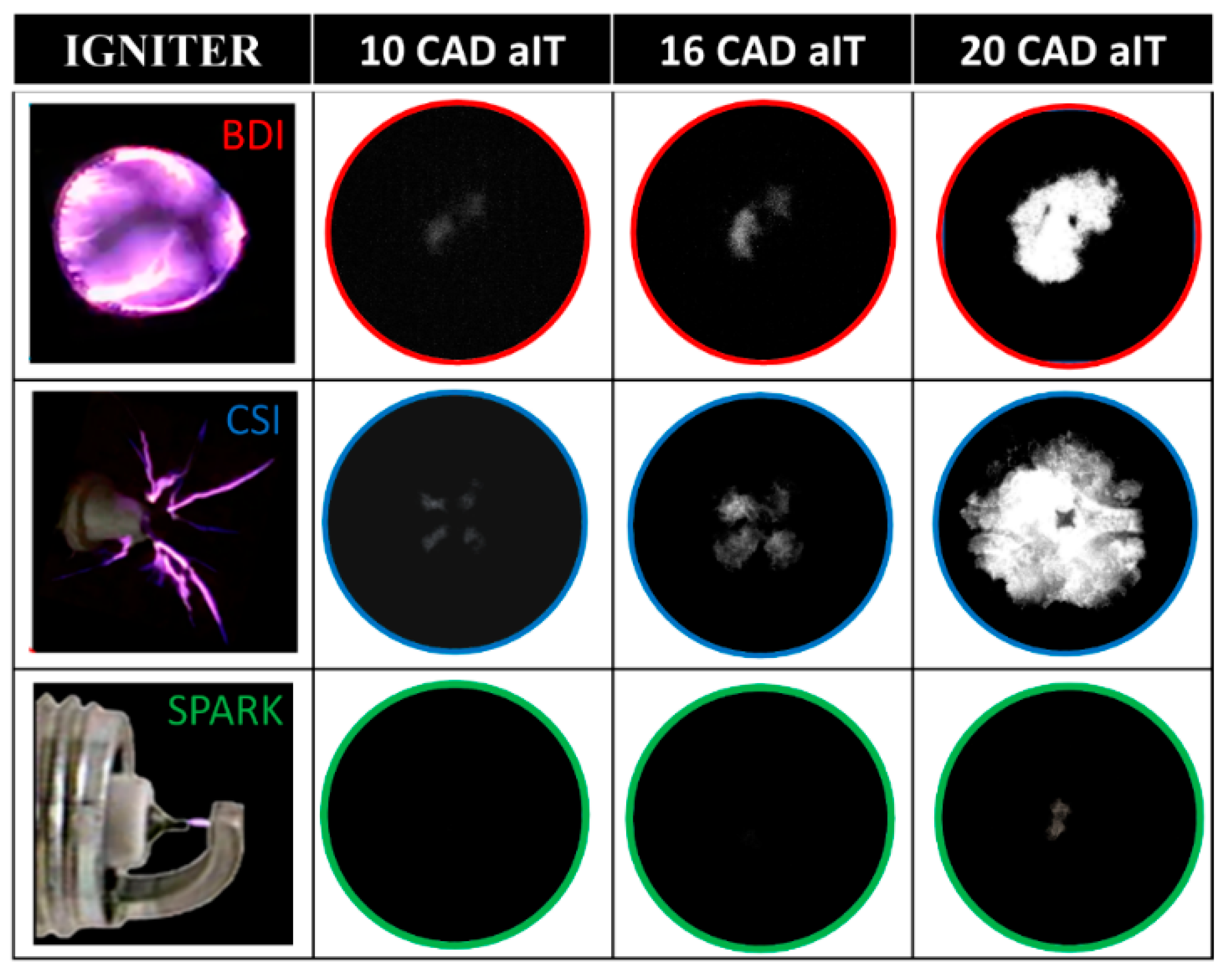
2.3. Igniters
3. Methods
3.1. Base Reference Algorithm
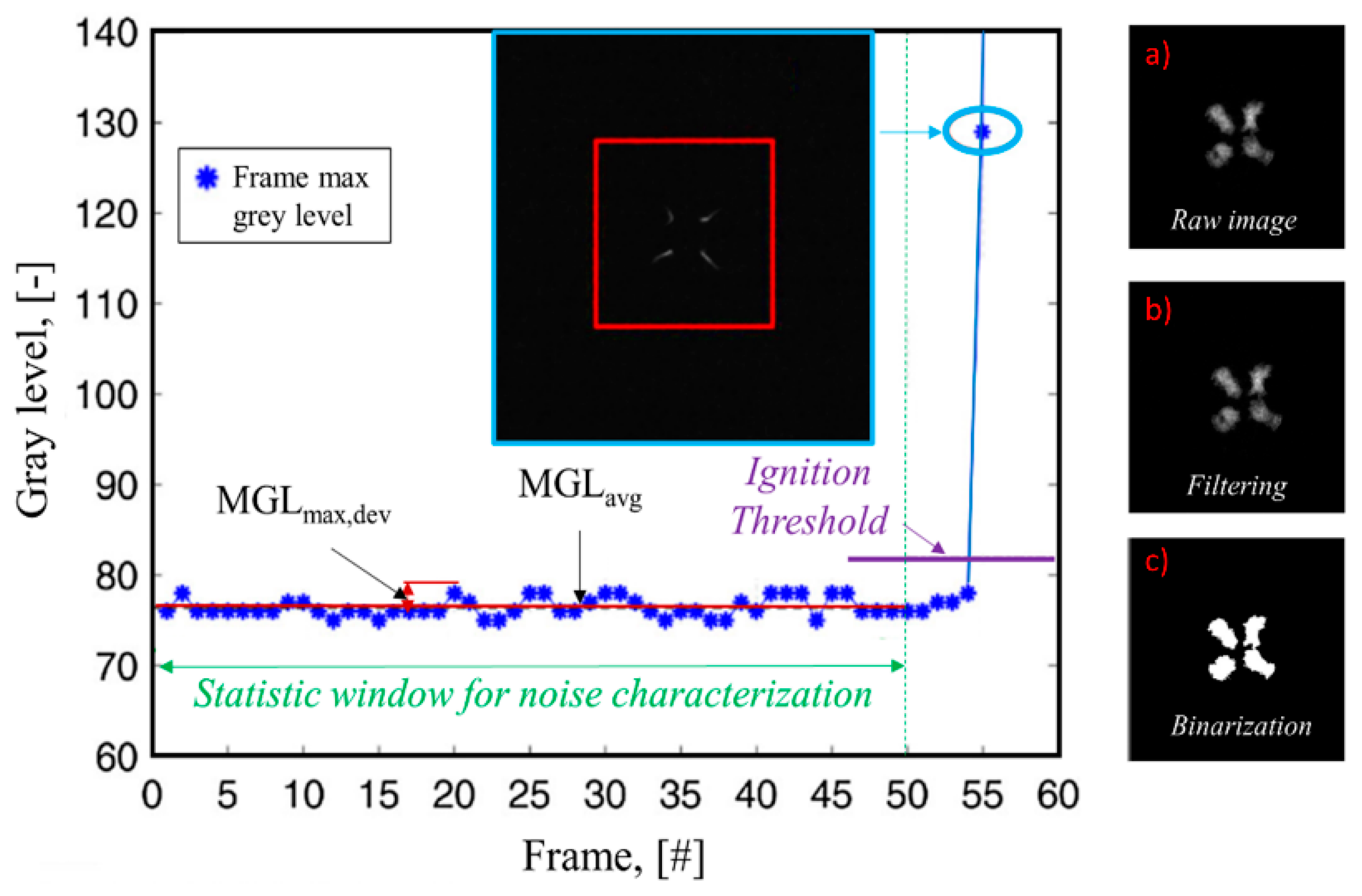
- Filtering—the filtering process is carried out on each recorded image by means of a 3 × 3 pixel median spatial filter, in order to reduce the salt and pepper noise. The filter is featured with variable dimension depending on images luminosity and contrast.
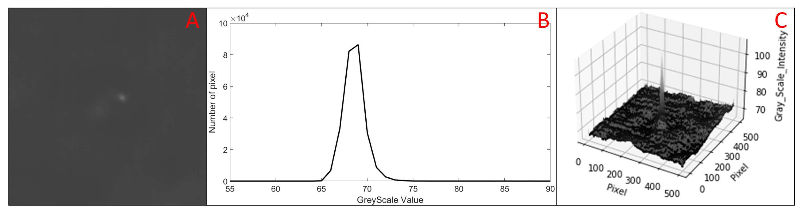
- Ignition Detection—Power-on detection is based on a frame-by-frame maximum gray level (MGL) detection on a centrally located sub-area of 220 × 220 pixel. The MGL of each frame is equal to the highest value recorded in such area. A statistically significant number of frames before switching on, i.e., 50, is chosen first and the average of the maximum gray level MGLavg (Equation (1)) in such windows is calculated, together with the maximum absolute deviation from the mean MGLmax,dev (Equation (2)) (Figure 5).
- 3.
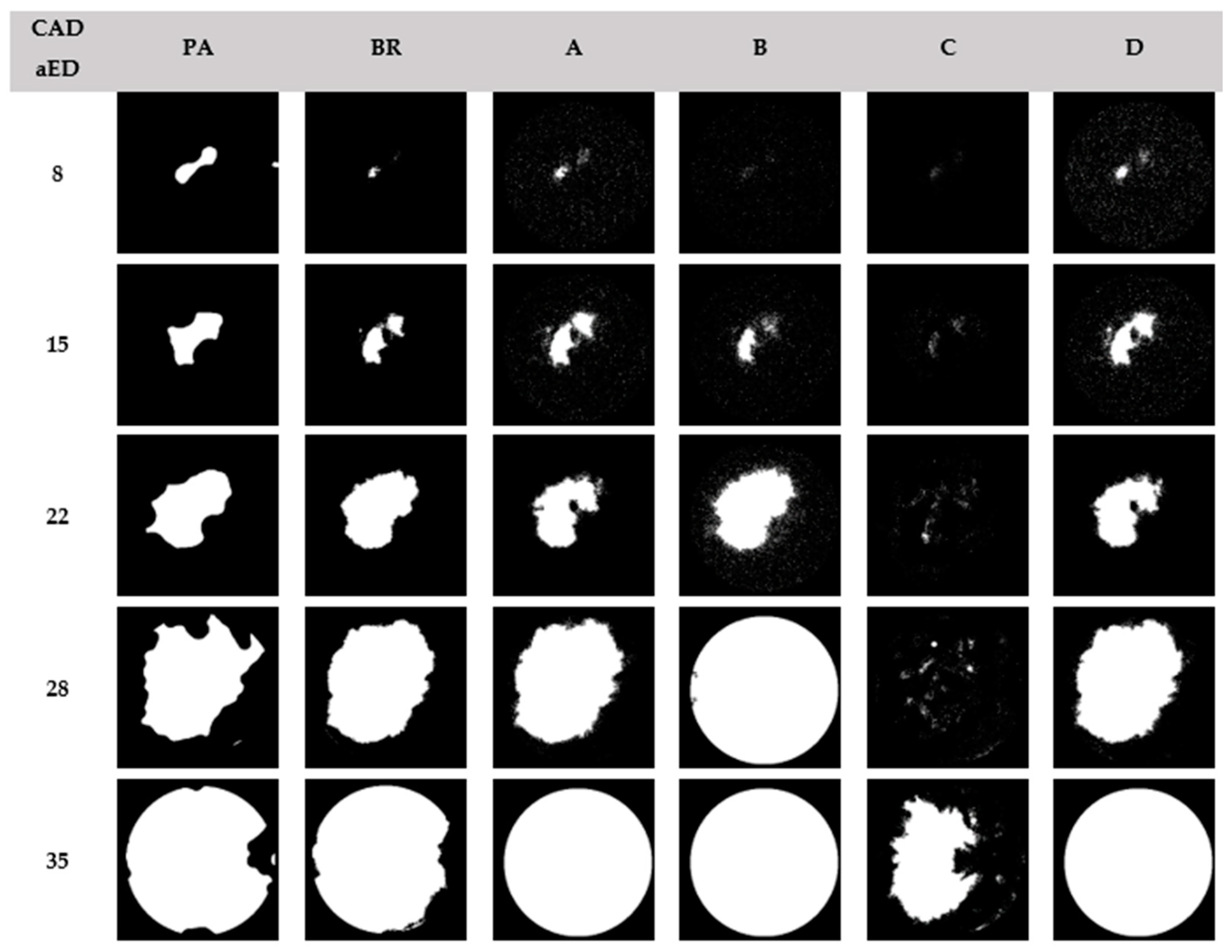
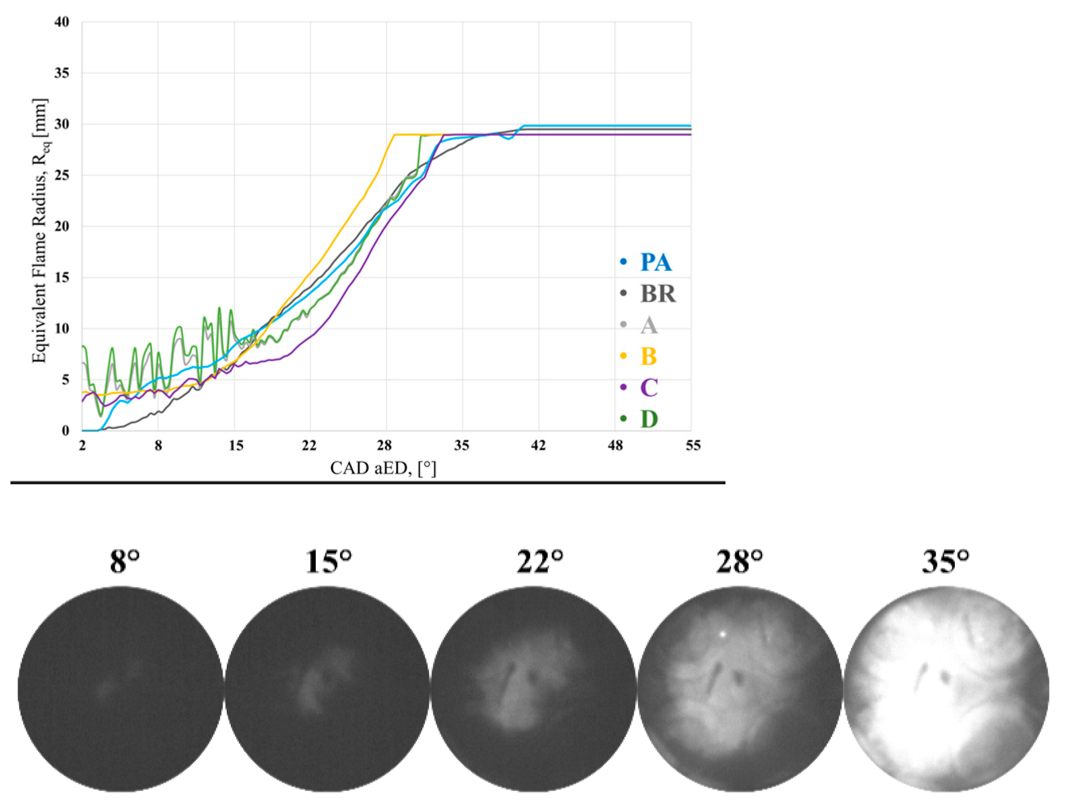
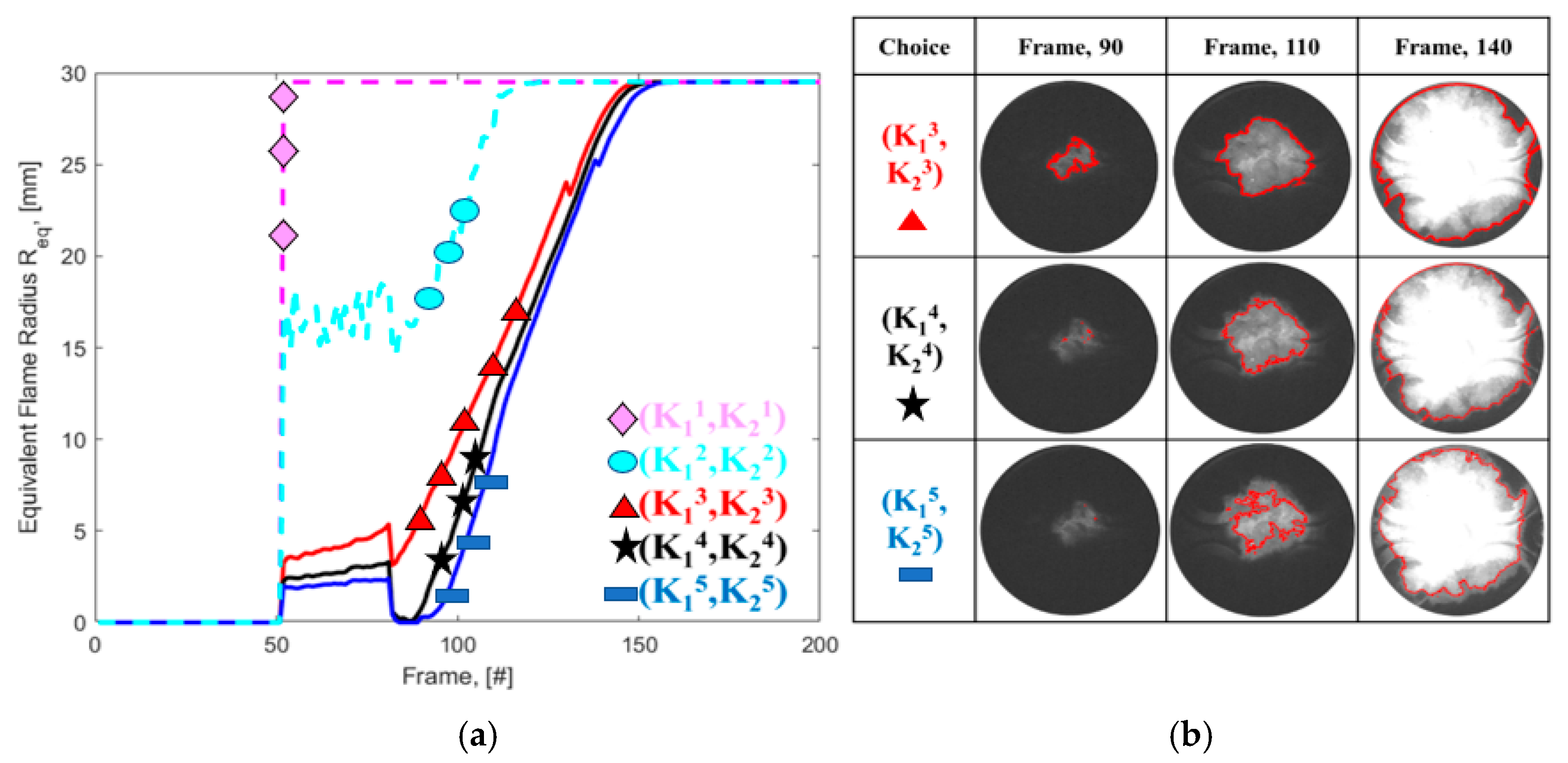
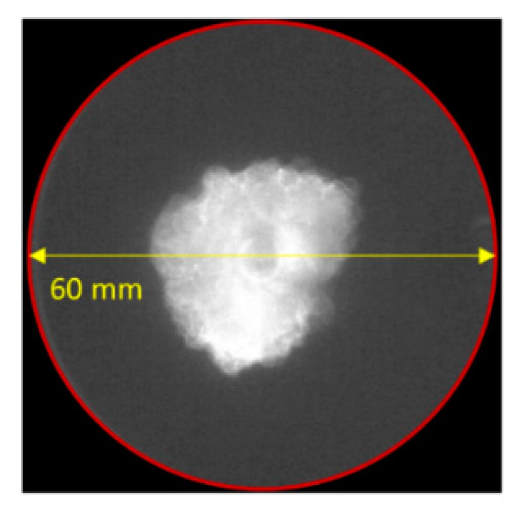
- Binarization—finally, a binarization of the image is carried out to convert from grayscale frames to black (unburned area) and white (burned area) ones with the aim to determine the equivalent flame radius Req (Equation (4)), starting from the knowledge of equivalent flame area Aeq. For each frame, Aeq in mm2 is obtained by computing the sum of the pixels representing the flame front (value equal to 1).
3.2. Proposed Algorithm
4. Test Campaign
5. Results and Discussion
6. Conclusions
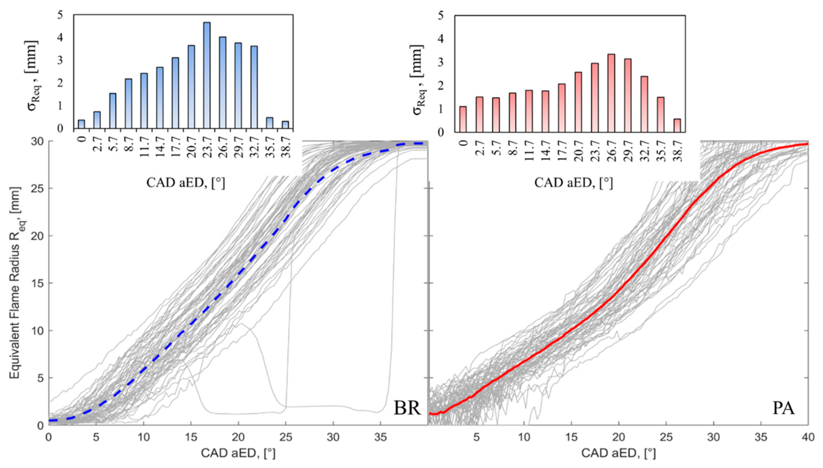
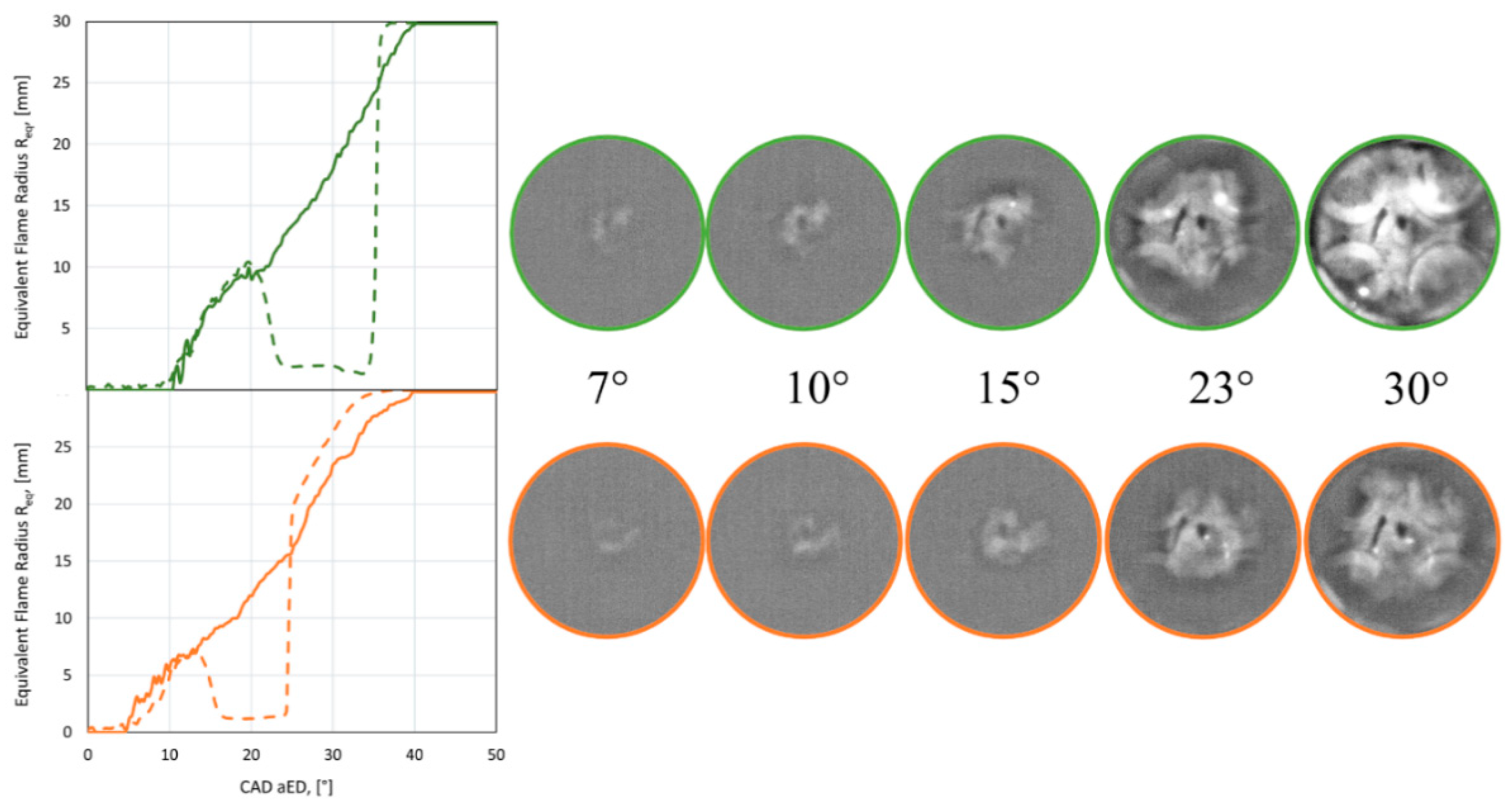
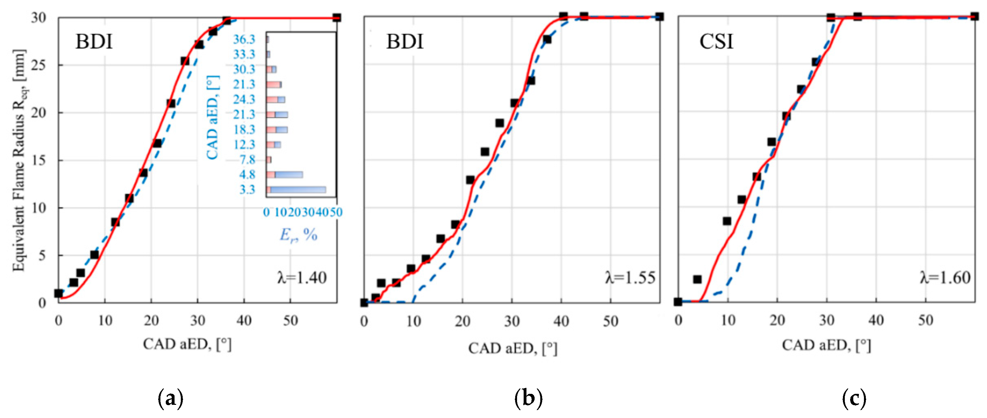
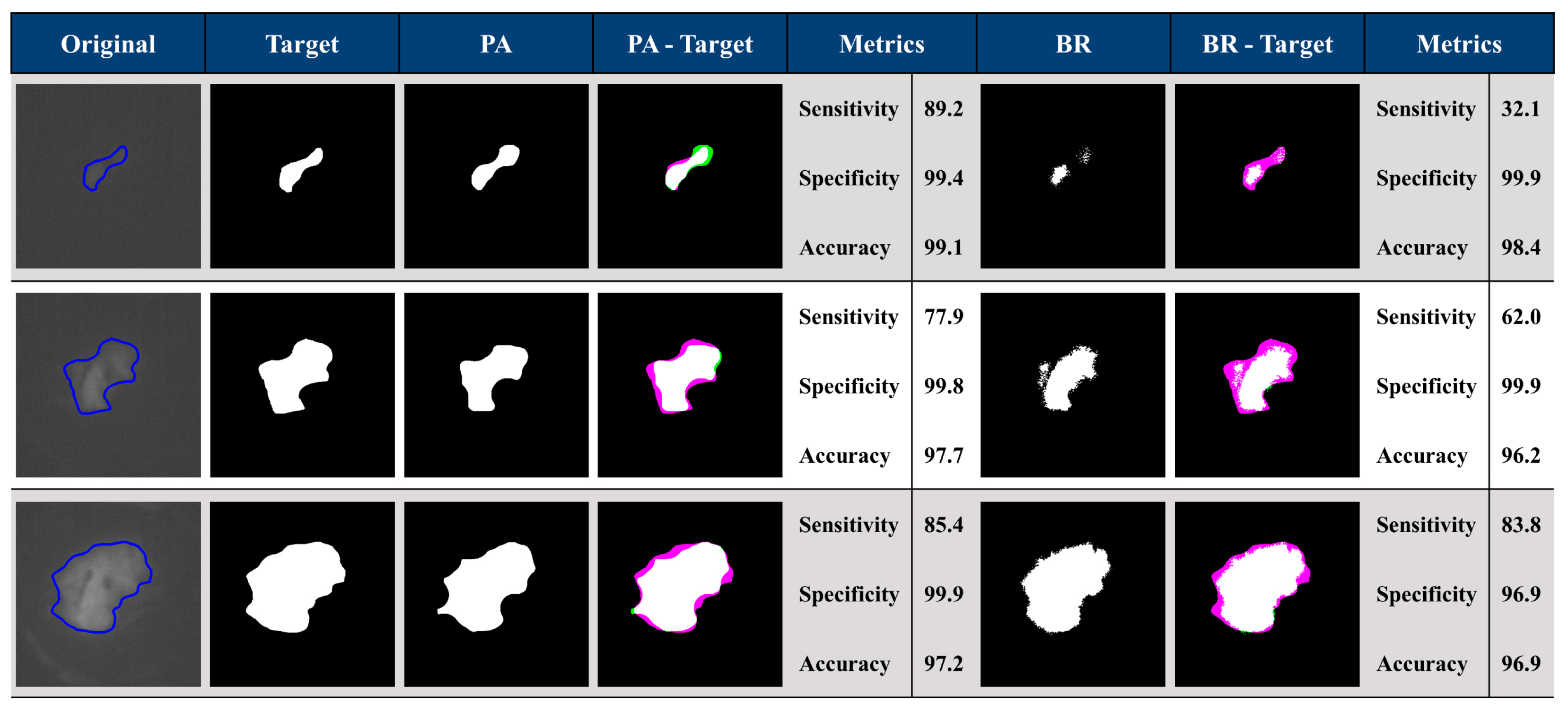
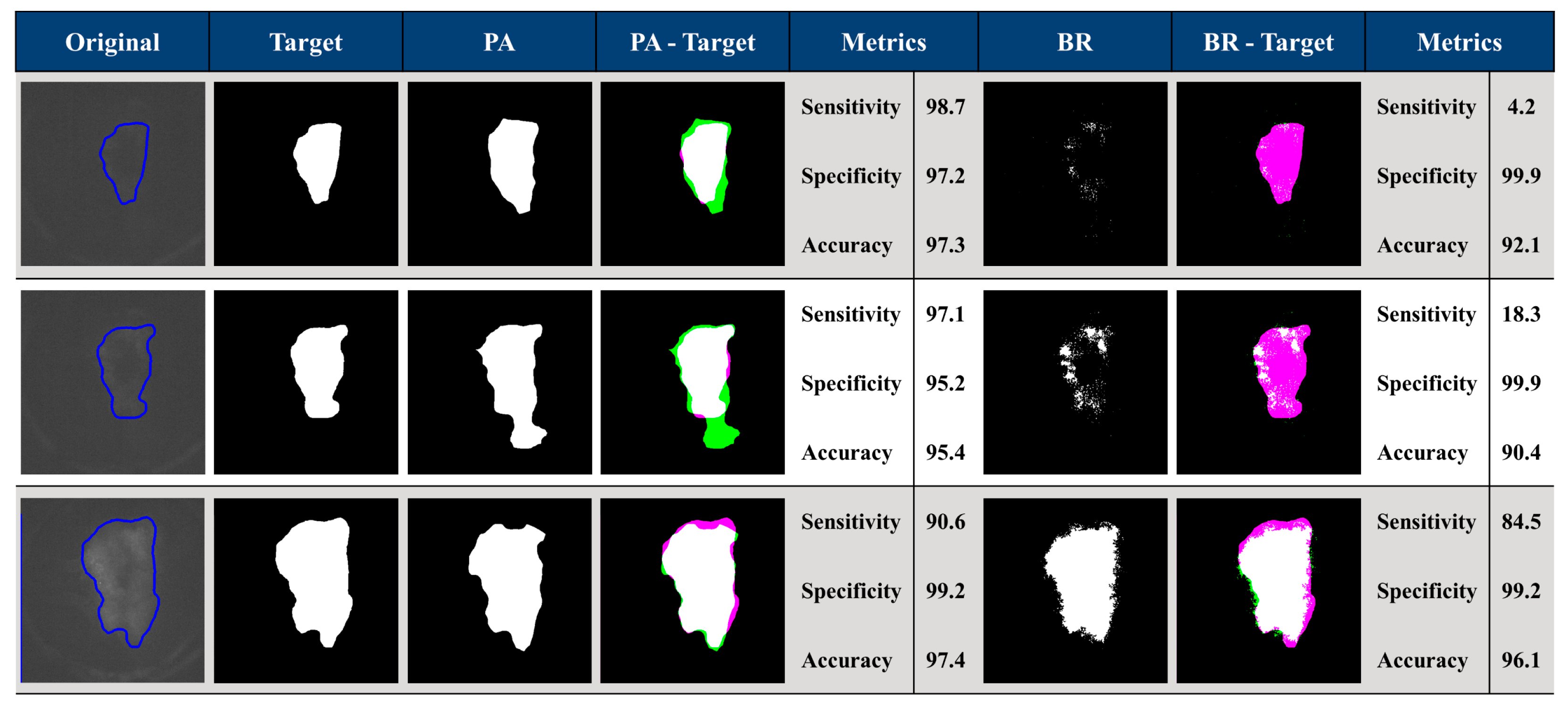
- Both algorithms were able to detect the flame front evolution by well reproducing the physical trend of the phenomenon. However, the PA curves bundles result in being less wide and therefore characterized by lower dispersion. Moreover, some combustions previously considered by the BR method as misfires or anomalies (3% of the total) are instead considered as physically valid by the proposed method. These features allow us to characterize the effective capability of the tested igniter on guarantying stable combustion onsets characterized by low cycle-to-cycle variability.
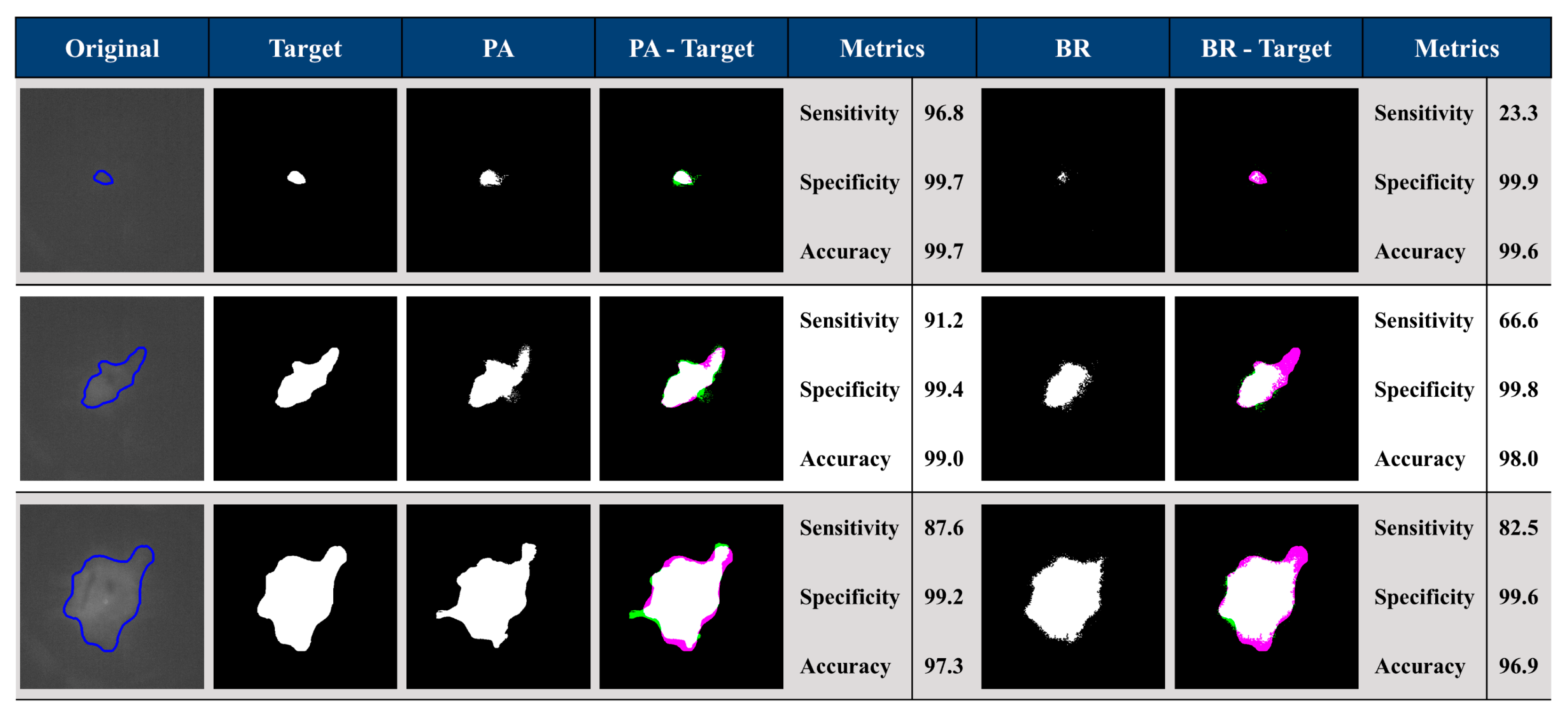
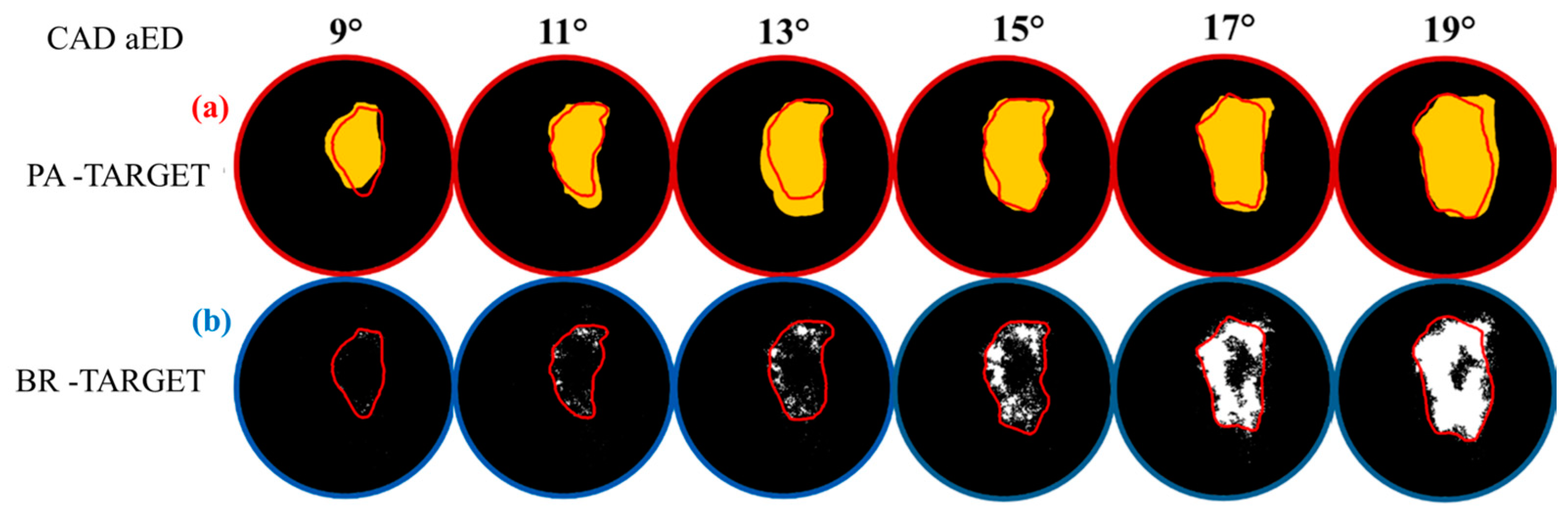
- In all cases analyzed, both methods were able to correctly reproduce the Target trend, and, in particular, PA showed a greater capability to detect in advance (up to 1500 μs), the kernel formation if compared to BR. In this way, it is possible to carry out a more detailed analysis of the igniter’s performance in the first moments of kernel formation. This feature is of pivotal importance at the leanest operating conditions of interest where BR showed its limits. Moreover, it allows for an almost-perfect correspondence between indicating and imaging analysis.
- The metric parameters confirmed the capability of PA to allow more reliable detection of early flame kernel development. The proposed algorithm performed values of Accuracy, Sensitivity, and Specificity higher on average if compared to the BR one. The darker the case, the higher the differences with the BR method, which makes the PA method more suitable for analyzing ultra-lean combustions, towards which automotive research is increasingly focused.
- Moreover, the capability of the PA algorithm to automatically estimate the binarization threshold allows us to perform an analysis of the flame front evolution completely independent from the user interpretation.
Author Contributions
Funding
Informed Consent Statement
Conflicts of Interest
Nomenclature
| ACIS | Advanced Corona Ignition System | IMEP | Indicated Mean Effective Pressure |
| aED | After End of Discharge | IT | Ignition Timing |
| AI | Artificial Intelligence | MBT | Maximum Brake Torque |
| BDI | Barrier Discharge Igniter | MFB | Mass Fraction Burned |
| BIMEF | Bio-Inspired Multi-Exposure Fusion | MFB50 | 50% of Mass Fraction Burned |
| BR | Base Reference method | ML | Machine Learning |
| CAD | Crank Angle Degree | OBD | On Board Diagnostic |
| CFD | Computational Fluid Dynamics | PFI | Port Fuel Injection |
| CNN | Convolutional Neural Network | PA | Proposed Algorithm |
| CoVIMEP | Covariance of IMEP | Req | Equivalent flame radius |
| CSI | Corona Streamer-Type igniter | RF | Radio Frequency |
| DI | Direct Injection | SI | Spark Ignition |
| ECU | Engine Control Unit | TDC | Top Dead Center |
| EGR | Exhaust Gas Recirculation | t on | Activation time of the igniter |
| FFDNet | Fast Flexible Denoising Network | TN | True Negative |
| FN | False Negative | TP | True Positive |
| FP | False Positive | Vd | Driving Voltage of the igniter |
| ICE | Internal Combustion Engine |
Appendix A
References
- Gao, J.; Tian, G.; Sorniotti, A.; Karci, A.E.; di Palo, R. Review of thermal management of catalytic converters to decrease engine emissions during cold start and warm up. Appl. Therm. Eng. 2019, 147, 177–187. [Google Scholar] [CrossRef]
- Alshammari, M.; Alshammari, F.; Pesyridis, A. Electric Boosting and Energy Recovery Systems for Engine Downsizing. Energies 2019, 12, 4636. [Google Scholar] [CrossRef] [Green Version]
- Merola, S.S.; Marchitto, L.; Tornatore, C.; Valentino, G.; Irimescu, A. UV-visible Optical Characterization of the Early Combustion Stage in a DISI Engine Fuelled with Butanol-Gasoline Blend. SAE Int. J. Engines 2013, 6, 2638. [Google Scholar] [CrossRef]
- Jeon, J.; Bock, N.; Northrop, W.F. In-cylinder Flame Luminosity Measured from a Stratified Lean Gasoline Direct Injection Engine. Results Eng. 2019, 1, 100005. [Google Scholar] [CrossRef]
- Sher, E.; Ben-Ya’ish, J.; Pokryvailo, A.; Spector, Y. A Corona Spark Plug System for Spark-Ignition Engines. SAE Tech. Pap. 1992, 920810. [Google Scholar] [CrossRef]
- Varma, A.; Thomas, S. Simulation, Design and Development of a High Frequency Corona Discharge Ignition System. SAE Tech. Pap. 2013, 1–10. [Google Scholar] [CrossRef]
- Burrows, J.; Mixell, K.; Reinicke, P.B.; Riess, M.; Sens, M. Corona ignition—Assessment of physical effects by pressure chamber, rapid compression machine, and single cylinder engine testing. In Proceedings of the 2nd International Conference on Ignition Systems for Gasoline Engines, Berlin, Germany, 24–25 November 2014. [Google Scholar]
- Mariani, A.; Foucher, F. Radio frequency spark plug: An ignition system for modern internal combustion engines. Appl. Energy 2014, 122, 151–161. [Google Scholar] [CrossRef]
- Starikovskii, A.Y.; Anikin, N.B.; Kosarev, I.N.; Mintoussov, E.I. Nanosecond Pulsed Discharges for Plasma Assisted Combustion and Aerodynamics. J. Propuls. Power 2008, 24, 1182–1197. [Google Scholar] [CrossRef]
- Sevik, J.; Wallner, T.; Pamminger, M.; Scarcelli, R. Extending Lean and Exhaust Gas Recirculation-Dilute Operating Limits of a Modern Gasoline Direct-Injection Engine Using a Low-Energy Transient Plasma Ignition System. J. Eng. Gas Turbines Power 2016, 138, 112807. [Google Scholar] [CrossRef]
- Ikeda, Y.; Padala, S.; Makita, M.; Nishiyama, A. Development of Innovative Microwave Plasma Ignition System with Compact Microwave Discharge Igniter. SAE Tech. Pap. 2015, 7. [Google Scholar] [CrossRef]
- Idicheria, C.A.; Najt, P.M. Potential of Advanced Corona Ignition System (ACIS) for future engine applications. In International Conference on Ignition Systems for Gasoline Engines; Springer International Publishing: Cham, Switzerland, 2017; pp. 315–331. [Google Scholar] [CrossRef]
- Marko, F.; König, G.; Schöffler, T.; Bohne, S.; Dinkelacker, F. Comparative optical and thermodynamic investigations of high frequency corona- and spark-ignition on a CV natural gas research engine operated with charge dilution by exhaust gas re- circulation. In International Conference on Ignition Systems for Gasoline Engines; Springer International Publishing: Cham, Switzerland, 2017; pp. 293–314. [Google Scholar] [CrossRef]
- Cruccolini, V.; Discepoli, G.; Ricci, F.; Petrucci, L.; Grimaldi, C.; Papi, S.; Dal Re, M. Comparative Analysis between a Barrier Discharge Igniter and a Streamer-Type Radio-Frequency Corona Igniter in an Optically Accessible Engine in Lean Operating Conditions. SAE Tech. Pap. 2020, 12. [Google Scholar] [CrossRef]
- Ricci, F.; Petrucci, L.; Cruccolini, V.; Discepoli, G.; Grimaldi, C.N.; Papi, S. Investigation of the Lean Stable Limit of a Barrier Discharge Igniter and of a Streamer-Type Corona Igniter at Different Engine Loads in a Single-Cylinder Research Engine. Multidiscip. Digit. Publ. Inst. Proc. 2020, 58, 11. [Google Scholar] [CrossRef]
- Ricci, F.; Zembi, J.; Battistoni, M.; Grimaldi, C.; Discepoli, G. Experimental and Numerical Investigations of the Early Flame Development Produced by a Corona Igniter; SAE Technical Paper 2019; SAE International: Warrendale, PA, USA, 2019. [Google Scholar] [CrossRef]
- Fiifi, R.; Yan, F.; Kamal, M.; Ali, A.; Hu, J. Engineering Science and Technology, an International Journal Artificial neural network applications in the calibration of spark-ignition engines: An overview. Eng. Sci. Technol. Int. J. 2016, 19, 1346–1359. [Google Scholar] [CrossRef] [Green Version]
- Çay, Y.; Çiçek, A.; Kara, F.; Saǧiroǧlu, S. Prediction of engine performance for an alternative fuel using artificial neural network. Appl. Therm. Eng. 2012, 37, 217–225. [Google Scholar] [CrossRef]
- Atkinson, C.M. Virtual Sensing: A Neural Network-based Intelligent Performance and Emissions Prediction System for On-Board Diagnostics and Engine Control. Prog. Technol. 1998, 73, 2–4. [Google Scholar]
- Pai, P.S.; Rao, B.R.S. Artificial Neural Network based prediction of performance and emission characteristics of a variable compression ratio CI engine using WCO as a biodiesel at different injection timings. Appl. Energy 2011, 88, 2344–2354. [Google Scholar] [CrossRef]
- Arsie, I.; Cricchio, A.; de Cesare, M.; Lazzarini, F.; Pianese, C.; Sorrentino, M. Neural network models for virtual sensing of NOx emissions in automotive diesel engines with least square-based adaptation. Control. Eng. Pract. 2017, 61, 11–20. [Google Scholar] [CrossRef]
- Rahimi Molkdaragh, R.; Jafarmadar, S.; Khalilaria, S.; Soukht Saraee, H. Prediction of the performance and exhaust emissions of a compression ignition engine using a wavelet neural network with a stochastic gradient algorithm. Energy 2018, 142, 1128–1138. [Google Scholar] [CrossRef]
- Warey, A.; Gao, J. Prediction of Engine-Out Emissions Using Deep Convolutional Neural Networks. SAE Tech. Pap. 2021, 3, 2863–2871. [Google Scholar]
- Salman, H.; Grover, J.; Shankar, T. Hierarchical Reinforcement Learning for Sequencing Behaviors. Neural Comput. 2018, 2733, 2709–2733. [Google Scholar] [CrossRef]
- Simonyan, K.; Vedaldi, A.; Zisserman, A. Deep inside convolutional networks: Visualising image classification models and saliency maps. In Proceedings of the 2nd International Conference on Learning Representations, ICLR 2014—Workshop Track Proceedings, Banff, AB, Canada, 14–16 April 2014; pp. 1–8. [Google Scholar]
- Soria, X.; Riba, E.; Sappa, A. Dense extreme inception network: Towards a robust CNN model for edge detection. In Proceedings of the 2020 IEEE Winter Conference on Applications of Computer Vision, WACV, Snowmass Village, CO, USA, 1–5 March 2020; pp. 1912–1921. [Google Scholar] [CrossRef]
- He, J.; Zhang, S.; Yang, M.; Shan, Y.; Huang, T. Bi-directional cascade network for perceptual edge detection. In Proceedings of the IEEE Computer Society Conference on Computer Vision and Pattern Recognition, Long Beach, CA, USA, 15–20 June 2019; pp. 3823–3832. [Google Scholar] [CrossRef] [Green Version]
- Gai, S.; Bao, Z. New image denoising algorithm via improved deep convolutional neural network with perceptive loss. Expert Syst. Appl. 2019, 138, 112815. [Google Scholar] [CrossRef]
- Shahdoosti, H.R.; Rahemi, Z. Edge-preserving image denoising using a deep convolutional neural network. Signal Processing 2019, 159, 20–32. [Google Scholar] [CrossRef]
- Shawal, S.; Goschutz, M.; Schild, M.; Kaiser, S.; Neurohr, M.; Pfeil, J.; Koch, T. High-speed imaging of early flame growth in spark-ignited engines using different imaging systems via endoscopic and full optical access. SAE Int. J. Engines 2016, 9, 704–718. [Google Scholar] [CrossRef]
- Bhatti, S.S.; Verma, S.; Tyagi, S.K. Energy and Exergy Based Performance Evaluation of Variable Compression Ratio Spark Ignition Engine Based on Experimental Work. Therm. Sci. Eng. Prog. 2019, 9, 332–339. [Google Scholar] [CrossRef]
- Irimescu, A.; Tornatore, C.; Marchitto, L.; Merola, S.S. Compression Ratio and Blow-by Rates Estimation Based on Motored Pressure Trace Analysis for an Optical Spark Ignition Engine. Appl. Therm. Eng. 2013, 61, 101–109. [Google Scholar] [CrossRef]
- SAE J1832_200102; Low Pressure Gasoline Fuel Injector, SAE International Standard. SAE International: Warrendale, PA, USA, 2001. [CrossRef]
- Ricci, F.; Cruccolini, V.; Discepoli, G.; Petrucci, L.; Grimaldi, C.; Papi, S. Luminosity and thermal energy measurement and comparison of a dielectric barrier discharge in an optical pressure-based calorimeter at engine relevant conditions. SAE Tech. Pap. 2021, 11. [Google Scholar]
- Romani, L.; Bianchini, A.; Vichi, G.; Bellissima, A.; Ferrara, G. Experimental Assessment of a Methodology for the Indirect in-Cylinder Pressure Evaluation in Four-Stroke Internal Combustion Engines. Energies 2018, 11, 1982. [Google Scholar] [CrossRef] [Green Version]
- Cruccolini, V.; Discepoli, G.; Cimarello, A.; Battistoni, M.; Mariani, F.; Grimaldi, C.N.; Dal Re, M. Lean combustion analysis using a corona discharge igniter in an optical engine fueled with methane and a hydrogen-methane blend. Fuel 2020, 259, 116290. [Google Scholar] [CrossRef]
- Cimarello, A.; Grimaldi, C.N.; Mariani, F.; Battistoni, M.; Dal Re, M. Analysis of RF Corona Ignition in Lean Operating Conditions Using an Optical Access Engine. SAE Tech. Pap. 2017. [Google Scholar] [CrossRef]
- Idicheria, C.A.; Yun, H.; Najt, P.M. An Advanced Ignition System for High Efficiency Engines. In Proceedings of the Ignition Systems for Gasoline Engines: 4th International Conference, Berlin, Germany, 6–7 December 2018; pp. 40–54. [Google Scholar] [CrossRef]
- Pineda, D.I.; Wolk, B.; Chen, J.-Y.; Dibble, R.W. Application of Corona Discharge Ignition in a Boosted Direct-Injection Single Cylinder Gasoline Engine: Effects on Combustion Phasing, Fuel Consumption, and Emissions. SAE Int. J. Engines 2016, 9, 1970–1988. [Google Scholar] [CrossRef]
- Discepoli, G.; Cruccolini, V.; Ricci, F.; di Giuseppe, A.; Papi, S.; Grimaldi, C.N. Experimental characterisation of the thermal energy released by a Radio-Frequency Corona Igniter in nitrogen and air. Appl. Energy 2020, 263, 114617. [Google Scholar] [CrossRef] [Green Version]
- Cruccolini, V.; Grimaldi, C.N.; Discepoli, G.; Ricci, F.; Petrucci, L.; Papi, S. An Optical Method to Characterize Streamer Variability and Streamer-to-Flame Transition for Radio-Frequency Corona Discharges. Appl. Sci. 2020, 10, 2275. [Google Scholar] [CrossRef] [Green Version]
- Ying, Z.; Li, G.; Gao, W. A bio-inspired multi-exposure fusion framework for low-light image enhancement. arXiv 2017, arXiv:1711.00591. [Google Scholar]
- Guo, X. LIME: A method for low-light image enhancement. In Proceedings of the 2016 ACM Multimedia Conference, Amsterdam, The Netherlands, 15–19 October 2016; pp. 87–91. [Google Scholar] [CrossRef]
- He, X.; Cai, D.; Yan, S.; Zhang, H.-J. Neighborhood Preserving Embedding. In Proceedings of the Tenth IEEE International Conference on Computer Vision (ICCV’05) Volume 1, Beijing, China, 17–21 October 2005; Volume 2, pp. 1208–1213. [Google Scholar] [CrossRef]
- Li, B.; Peng, X.; Wang, Z.; Xu, J.; Feng, D. (AOD-Net)—AOD-Net:All-in-one dehazing network boyi. In Proceedings of the IEEE International Conference on Computer Vision (ICCV), Venice, Italy, 22–29 October 2017; pp. 4770–4778. [Google Scholar]
- Wang, Z.; Bovik, A.C.; Sheikh, H.R.; Simoncelli, E.P. Image quality assessment: From error visibility to structural similarity. IEEE Trans. Image Processing 2004, 13, 600–612. [Google Scholar] [CrossRef] [PubMed] [Green Version]
- Horé, A.; Ziou, D. Image quality metrics: PSNR vs. SSIM. In Proceedings of the International Conference on Pattern Recognition, Istanbul, Turkey, 23–26 August 2010; pp. 2366–2369. [Google Scholar] [CrossRef]
- Zhang, K.; Zuo, W.; Zhang, L. FFDNet: Toward a fast and flexible solution for CNN-Based image denoising. IEEE Trans. Image Processing 2018, 27, 4608–4622. [Google Scholar] [CrossRef] [Green Version]
- Islam, M.Z.; Islam, M.M.; Asraf, A. A combined deep CNN-LSTM network for the detection of novel coronavirus (COVID-19) using X-ray images. Inform. Med. Unlocked 2020, 20, 100412. [Google Scholar] [CrossRef]


| Feature | Value | Unit |
|---|---|---|
| Image resolution | 512 × 512 | pixel |
| Sampling rate | 20 | kHz |
| Exposure time | 49 | μs |
| Bit depth | 8 | bit |
| Spatial resolution | 124 | μm/pixel |
| Temporal resolution (@1000 rpm) | 0.3 | CAD/frame |
| Cases | Sequences |
|---|---|
| A | BIMEF |
| B | DEHAZING |
| C | BIMEF+DEHAZING |
| D | DEHAZING + BIMEF |
| E | BIMEF+DEHAZING+DENOISING |
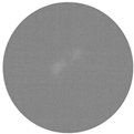
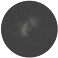
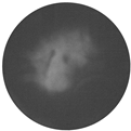
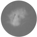
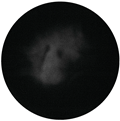
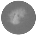
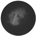
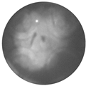
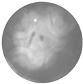
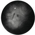
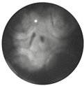
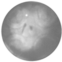
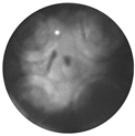
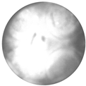
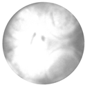
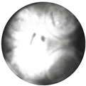
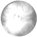
| CAD aED | Original Frames | A | B | C | D | E | ||||||
|---|---|---|---|---|---|---|---|---|---|---|---|---|
| SSIM | PSNR | SSIM | PSNR | SSIM | PSNR | SSIM | PSNR | SSIM | PSNR | |||
| 8 | 0.76 | 11.6 | 0.42 | 14.1 | 0.84 | 31.6 | 0.40 | 11.3 | 0.95 | 35.5 | ||
 |  |  |  |  | 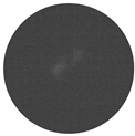 | |||||||
| 15 | 0.78 | 11.6 | 0.44 | 13.8 | 0.85 | 32.7 | 0.41 | 11.4 | 0.95 | 38.1 | ||
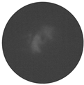 |  |  |  |  |  | |||||||
| 22 | 0.89 | 15.3 | 0.49 | 13.2 | 0.84 | 21.6 | 0.47 | 15.4 | 0.93 | 21.7 | ||
 |  |  |  |  |  | |||||||
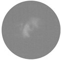
| 29 | 0.91 | 17.3 | 0.64 | 12.6 | 0.87 | 19.8 | 0.48 | 17.3 | 0.92 | 19.8 | ||
 |  |  |  |  |  | |||||||
| 36 | 0.92 | 21.2 | 0.82 | 14.7 | 0.89 | 20.8 | 0.6 | 21.7 | 0.93 | 21.9 | ||
 |  |  |  |  |  | |||||||
| Igniter Type | Engine Speed, (pm) | λ, (-) | Vd, (V) | ton, (μs) | IT, (CAD aTDC) | IMEP, (bar) | COVIMEP, (%) |
|---|---|---|---|---|---|---|---|
| BDI | 1000 | 1.4 | 60 | 1500 | −36 | 3.6 | 1.5 |
| BDI | 1.55 | 60 | 1000 | −53 | 3.2 | 2.3 | |
| CSI | 1.6 | 17 | 1000 | −47 | 3.1 | 3 |
Publisher’s Note: MDPI stays neutral with regard to jurisdictional claims in published maps and institutional affiliations. |
© 2022 by the authors. Licensee MDPI, Basel, Switzerland. This article is an open access article distributed under the terms and conditions of the Creative Commons Attribution (CC BY) license (https://creativecommons.org/licenses/by/4.0/).
Share and Cite
Petrucci, L.; Ricci, F.; Mariani, F.; Discepoli, G. A Development of a New Image Analysis Technique for Detecting the Flame Front Evolution in Spark Ignition Engine under Lean Condition. Vehicles 2022, 4, 145-166. https://doi.org/10.3390/vehicles4010010
Petrucci L, Ricci F, Mariani F, Discepoli G. A Development of a New Image Analysis Technique for Detecting the Flame Front Evolution in Spark Ignition Engine under Lean Condition. Vehicles. 2022; 4(1):145-166. https://doi.org/10.3390/vehicles4010010
Chicago/Turabian StylePetrucci, Luca, Federico Ricci, Francesco Mariani, and Gabriele Discepoli. 2022. "A Development of a New Image Analysis Technique for Detecting the Flame Front Evolution in Spark Ignition Engine under Lean Condition" Vehicles 4, no. 1: 145-166. https://doi.org/10.3390/vehicles4010010
APA StylePetrucci, L., Ricci, F., Mariani, F., & Discepoli, G. (2022). A Development of a New Image Analysis Technique for Detecting the Flame Front Evolution in Spark Ignition Engine under Lean Condition. Vehicles, 4(1), 145-166. https://doi.org/10.3390/vehicles4010010