1. Introduction
In the late 1970s, the European Union (EU) established the link between air quality and automotive emissions, thereby setting in motion policies to reduce air pollution. In 1992, the Euro norm for passenger cars was introduced that set a ceiling for concentration of pollutants [
1]. These norms are made more stringent with time [
2] and enforces companies to adopt more efficient automotive powertrains. This can be illustrated with the growth in hybrid electric vehicle (HEV) market share and the estimated increase in sales over the next decade [
3]. In line with the efforts to improve overall powertrain efficiency, significant strides have been made in transmission development. As a result, the continuously variable transmission (CVT) with a steel pushbelt is predicted to achieve an efficiency of 97% [
4].
Based on these automotive trends and the superiority of HEV topology P2 over P1 [
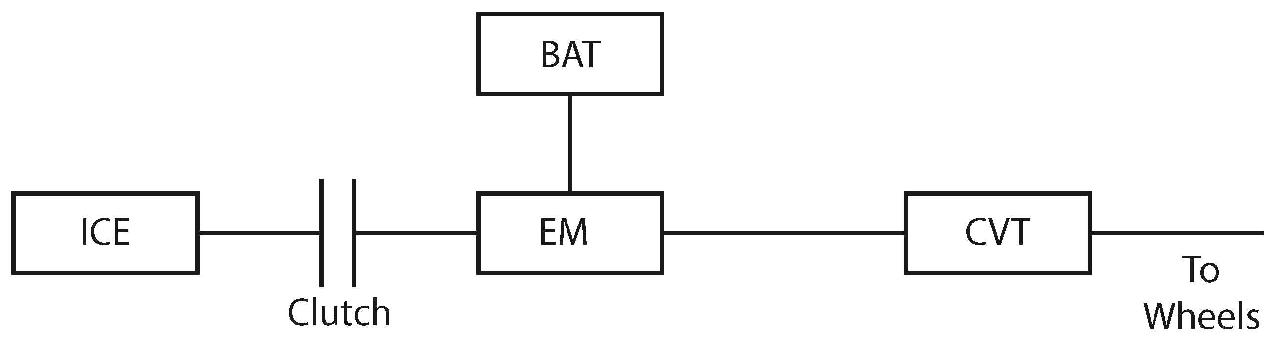
5], a P2 plug-in hybrid electric vehicle (PHEV) with a CVT is considered as the system, wherein an electric motor (EM) is directly connected to the drive shaft while the internal combustion engine (ICE) is connected in parallel via a clutch, depicted in
Figure 1. An energy source, in this case a battery (BAT), supplies power to the EM. The combined power from the EM and the ICE is transmitted by the CVT to the wheels, with an intermediate speed reduction through a fixed differential gear. The addition of an EM introduces a torque-split control variable that is strongly inter-coupled with the control of the transmission. Strategic control of the torque-split, transmission gear ratio, clutches, engine on/off, etc., can reduce the combined energy consumption of the EM and ICE. Several strategies exist that seek to minimize this energy consumption, and these strategies are reviewed in
Section 1.1.
1.1. Literature Review
The clutch in the P2 configuration disengages the ICE from the powertrain to reduce engine drag; however, it is not considered as a control variable in this study. The clutch is assumed to be activated when there is no demand for ICE power and while activated the ICE is assumed to be idling. Therefore, in this study, only the gear ratio and torque split are considered as control variables and the state of charge of BAT () is considered as the state of the system.
Accounting for the system dynamics, boundary conditions, constraints on states and control spaces, the two-point boundary value problem can be solved using dynamic programming (DP) that guarantees optimality through an exhaustive search of all control and state grids based on the Bellman’s principle of optimality [
6,
7]. With respect to the considered system, this implies that, for an a priori drive cycle with known boundary conditions, the optimal gear ratio and optimal torque split can be found offline using DP, thereby serving as a benchmark for all other control strategies. This optimal policy is drive cycle dependent, thereby rendering DP unsuitable for online implementation [
8]. Online-implementable control strategies exist; however, they are sub-optimal and generally decouple the control variables. Therefore, these online implementable control strategies are reviewed separately as gear ratio control for CVTs in
Section 1.1.1 and torque split control in
Section 1.1.2.
1.1.1. Gear Ratio Control
CVTs offer a wide range of gear ratios. The classical optimal operating line (OOL) strategy is found to be the most economical method for the conventional drive-train [
9]. Subsequently, a modified optimal operating line (M-OOL) strategy that accounts for the CVT system loss is shown to marginally improve over the OOL [
10]. A similar method using the equivalent consumption of the electric energy to fuel energy is used to build a hybrid optimal operation Line (H-OOL) [
11]. Apart from these standard rule-based methods, another method uses sub-optimal feedback controllers to approximate the optimal control policy and achieves almost optimal performance at a substantially reduced computational effort [
12].
1.1.2. Torque Split Control
A comprehensive review of torque split control strategies is given in [
13]. Common heuristic based control strategies can be divided into rule-based [
14] and fuzzy-logic approaches [
15,
16,
17]. Fuzzy-logic based approaches are preferred for their robustness and suitability to multi-domain, nonlinear, time-varying systems such as PHEVs [
13]. Model predictive control (MPC) methods are also found to be computationally efficient for online implementation [
18,
19]. However, MPC is heavily dependent on the prediction accuracy and therefore online optimization methods based on Pontryagin’s minimum principle (PMP) are preferred [
20,
21]. An added advantage of PMP is that it is governed by only one costate variable [
22]. Similar control strategies, like equivalent consumption minimization strategy (ECMS) first introduced in [
23], utilizes the efficiency of the battery and the operating mode to determine the equivalence factor. This ECMS was adapted to PMP [
24] and a comparative study with DP was done in [
25]. In principle, a good estimation of the costate or equivalence factor can result in near optimal performance [
26,
27] and therefore online optimization methods are preferred to heuristics [
28].
Meanwhile, machine learning (ML) techniques have gained popularity for their ability to control complex tasks by deriving patterns or rules from a data-set or through experience [
29,
30]. These techniques have also been extended to automotive applications, for example, drive cycle prediction [
31], drive cycle recognition [
32], training the torque split controller from DP using supervised machine learning (SML) [
33], reinforcement learning (RL) for power distribution between the battery and the capacitor [
34], etc. In certain tasks, controllers trained using ML have outperformed the controllers based on classical control theory [
35].
In the case of supervisory control strategies for an HEV, certain learning based strategies are shown to be comparable to the commonly used control strategies [
31]. For continuous-spaces, the actor–critic method was used for the power management in a PHEV [
36]. A qualitative study on RL techniques on HEVs and PHEVs shows potential for RL controllers to replace rule based controllers [
37]. Similarly, learning based techniques have been used to train neural networks to predict the driving environment and generate an optimal torque split, achieving fuel savings [
33]. However, further improvement can be made by customizing the strategy to a specific driving behavior as driving behavior can influence vehicle fuel consumption [
32,
38]. This driving behavior could be based on the geographic-location, traffic congestion, personal style, etc. In practice, automotive companies offer driving modes such as eco, sport, normal, etc., to address these driver preferences but cannot fully encapsulate the driving behavior. Therefore, the potential of ML can be exploited to bridge the gap to the global optimal without human intervention and thus forms the basis of this research.
Research Question: How can ML be incorporated into supervisory powertrain control in order to adapt to a specific driving behavior?
1.2. Objectives
Apart from the main objective of minimizing overall energy consumption, ML can be extended to improve upon existing practices. In the existing practices for HEVs and conventional powertrains, the control strategy is tuned by experienced calibration engineers through iterative real-time vehicle tests (calibration time) before online implementation, resulting in a strategy that caters to the average driver. Therefore, the objectives (
and
) of the study are to combat the drawbacks of conventional practices, i.e., calibration time and the inability to customize the control strategy to a specific driver. Furthermore, as suggested in literature [
37], RL methods can improve fuel economy when compared to the rule based methods. However, these RL techniques come at the cost of learning time and this forms the third objective (
), wherein the learning time must be minimized:
O1: customize the control strategy to a specific driver,
O2: reduce the time consumed for calibration,
O3: improve learning efficiency.
In order to address
, the controller must be able to account for the driver behavior. In this study, the vehicle velocity and its acceleration are considered as a representation of the driver behavior. In practice, the throttle position is considered; however, with a backward facing model, it is replaced with vehicle acceleration. In order to address
, a learning algorithm must be present to adapt to this driver behavior. Several algorithms are available that can learn in real-time or from past data and are discussed in
Section 1.1. Real-time learning algorithms like RL require an exploration phase (trial and error) to determine the optimal control respective to the vehicle state, which suggests that it needs to repeatedly encounter identical vehicle states in order to determine the best possible control. However, real-world driving will seldom encounter the identical vehicle states, i.e., identical combination of velocity, acceleration, state of charge, etc. Hence, real-time learning solutions could require thousands of kilometers of driving in order to learn a good control strategy. Objective
is to improve learning efficiency thereby reducing training time. In order to address
, it must be understood that for a given driving trajectory, with boundary conditions, there exists an optimal control policy. Therefore, utilizing this optimal control policy for training would reduce the training time drastically, as there is no requirement of an exploration phase. This would entail that the training occurs after the driving task is completed, in order to find and learn the optimal control policy.
1.3. Contributions
In this paper, a framework is presented that consists of three segments; in segment 1, the route planner analyzes the drive cycle and the end-point condition for the state of charge () is derived. Under the assumption that the drive cycle is representative of the driving behavior, is addressed. In segment 2, based on the end-point condition on the state of charge (), DP finds an optimal control policy for the a priori drive cycle. Finally, in segment 3, the input parameters from segment 1 and the optimal control policy from segment 2 are used to train a controller using SML algorithms. The absence of human intervention to learn a strategy that addresses and utilizes the optimal control policy that addresses .
This trained controller is validated by comparing its performance in terms of fuel consumption, to the global optimal solution derived from DP and an online-implementable control strategy based on literature that uses a combination of OOL and PMP. It should be noted that DP in this study refers to the approximate dynamic programming, wherein the state and control spaces are discretized.
Organization: The paper is organized as follows,
Section 2 describes the mathematical modeling of the system.
Section 3 formulates the control problem and introduces the proposed framework to solve the problem.
Section 4 elaborates on the experimental setup, discusses the results, and presents a test-case. Finally,
Section 5 concludes this study and suggests future propositions.
2. Modeling of the System
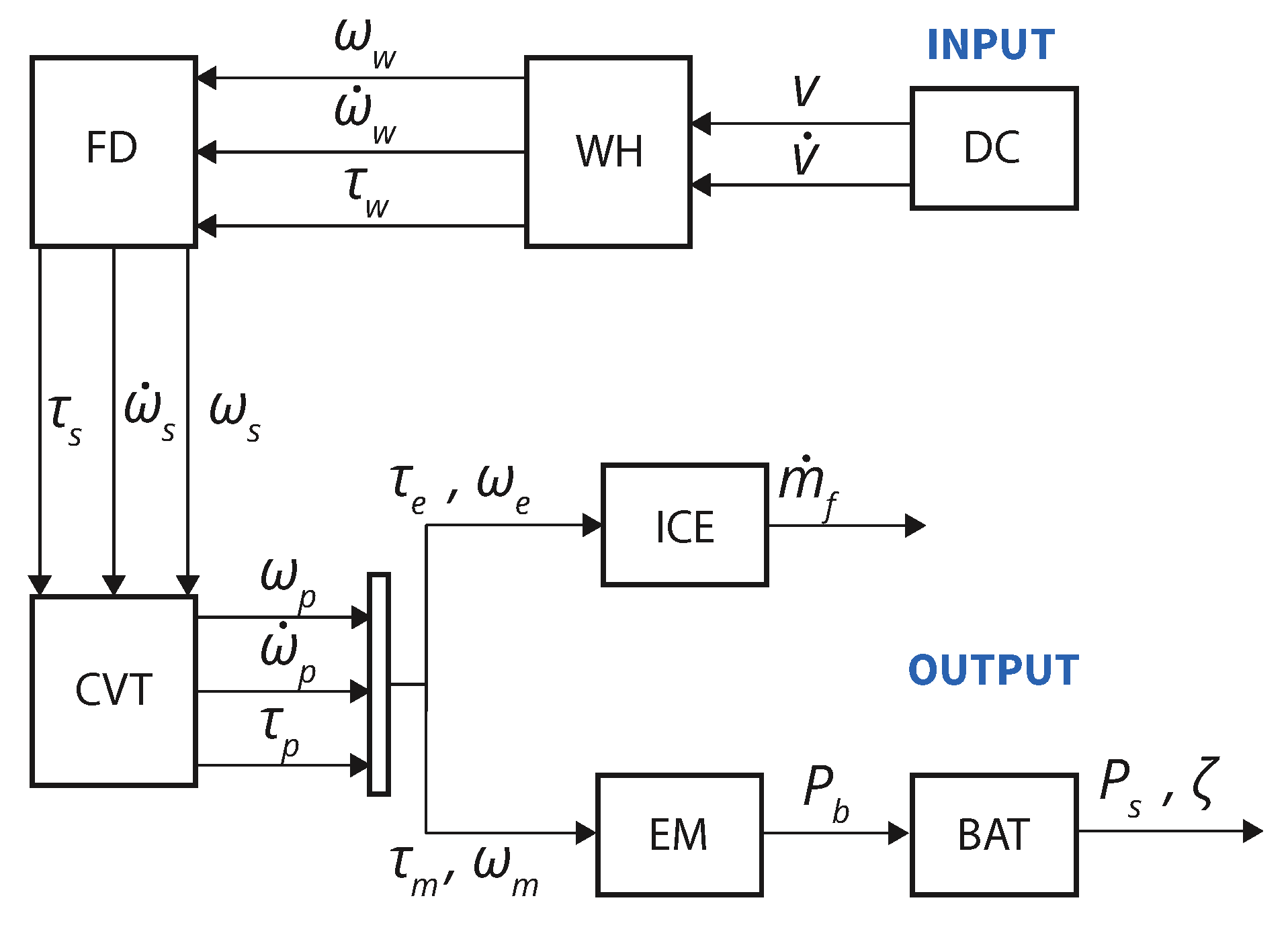
In this section, the HEV powertrain components are described and the energy flow illustrated in
Figure 1 is mathematically modeled. The system is modeled as backward quasi-static, which approximates the system to be static at a given time instance, depicted in
Figure 2. Only longitudinal dynamics of the vehicle are considered, and it is assumed that the vehicle only moves forward or is stationary. The equations are taken from [
39] and the parameter values are given in experimental design setup is
Section 4. Energy losses within each component are taken from manufacturer specifications or modeled from test-bench data.
Input parameters: The input to the system is the drivecycle, specifically the vehicle speed and the vehicle acceleration, recorded at 1 Hz. To physically achieve this acceleration at a given velocity, the resisting forces must be equal to the driving force applied by the wheel on the road. The resisting forces taken into account are aerodynamic drag (
), rolling resistance (
), gravity (
) and inertia (
), given respectively by Equations (
1)–(
4):
where
is the density of air,
is the aerodynamic coefficient,
is the frontal surface area,
v is the vehicle speed,
is the mass of the vehicle,
g is the acceleration due to gravity,
is the static rolling coefficient,
is the road inclination,
is the mass of rotating parts, and
is the acceleration of the vehicle.
Wheel: The driving force (
) required at the point of contact of the wheel with the road is the sum of the resisting forces. Subsequently, the torque of the wheel axle is calculated as a factor of the wheel radius. The wheel speed and wheel acceleration can be calculated from the vehicle speed and the vehicle acceleration respectively, as shown in Equations (
6) and (
7):
where
is the torque at the wheel axle,
is the radius of the wheel,
is the rotational speed of the wheel, and
is the rotational acceleration of the wheel.
Differential: The fixed differential factors in the fixed gear ratio, resulting in the required torque and rotational speed at the secondary pulley:
where
is the ratio of the fixed differential gear,
is the torque at the secondary pulley and
is the rotational speed of the secondary pulley.
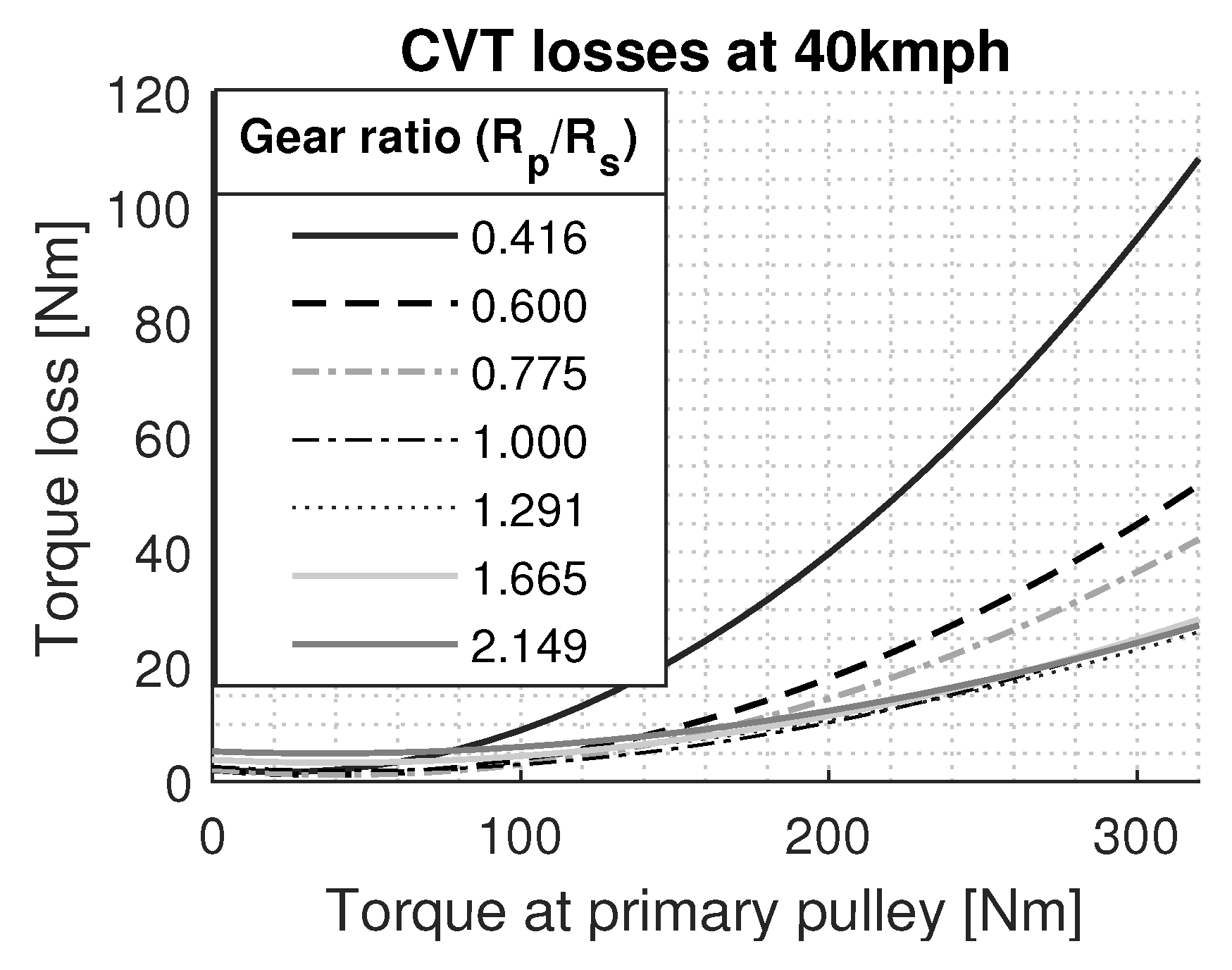
Gearbox: The gearbox used in this study is a push-belt CVT type P920 [
40], with an under-drive ratio of 0.416 and an over-drive ratio of 2.149. Transmission of speed and torque from the secondary pulley to the primary pulley is dependent on the selected gear ratio; this relation is shown in Equation (
11). The loss in transmission of power is attributed to the mechanical loss and pumping loss, modeled from experimental data [
40]. An example of the mechanical loss is illustrated in
Figure 3 for seven different gear ratios for the vehicle speed of 40 kmph. These losses are measured at the test-bench for the full range of gear ratios at various vehicle speeds and stored in a lookup-table:
where
is the torque at the primary pulley,
is the selected gear ratio of the CVT,
is the torque loss within the CVT that is the sum of the mechanical and pumping losses, and
is the rotational speed of the primary pulley.
Torque split: The torque at the primary pulley of the CVT is the combined torque delivered by the EM and ICE:
where
is the ICE torque and
is the EM torque
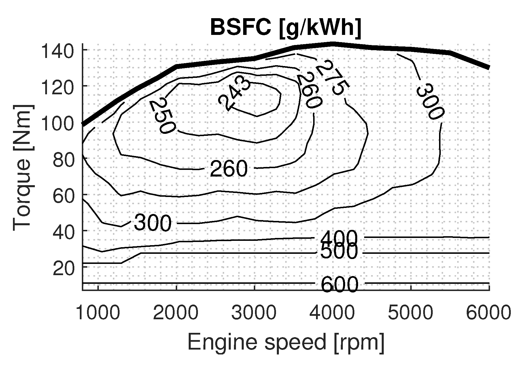
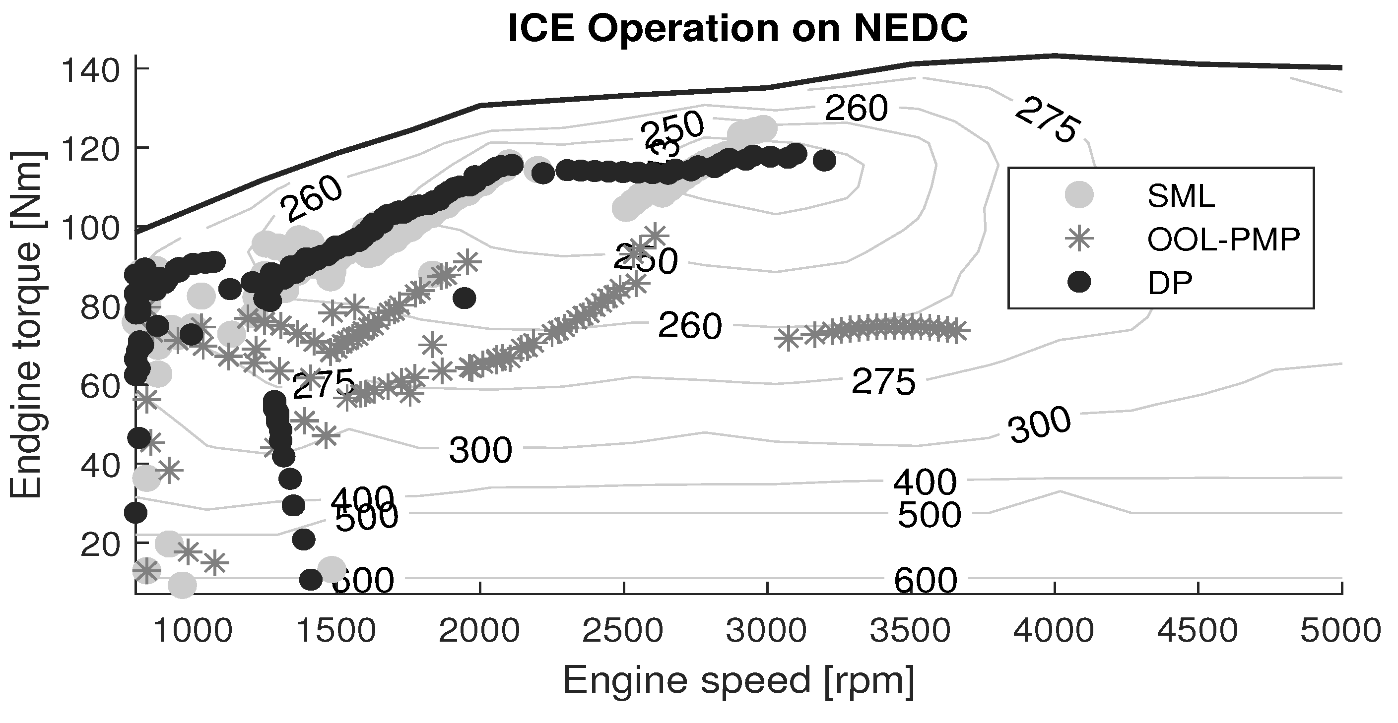
Engine: The ICE is a 1.6 L, 82-kW unit producing a maximum torque of 143-Nm and is taken from the Peugeot 206 model year 2005. The instantaneous ICE torque and speed are used to determine the fuel consumption from the brake specific fuel consumption (BSFC) map, depicted in
Figure 4. The BSFC map expresses the fuel consumed in [g/kWh] that is taken from the manufacturer’s specification and is converted to [g/s] using Equation (
13):
where
is the instantaneous fuel mass flow in [g/s], BSFC is the fuel consumed in [g/kWh],
is the ICE torque,
is the ICE rotational speed, and
is the fuel consumption at idling.
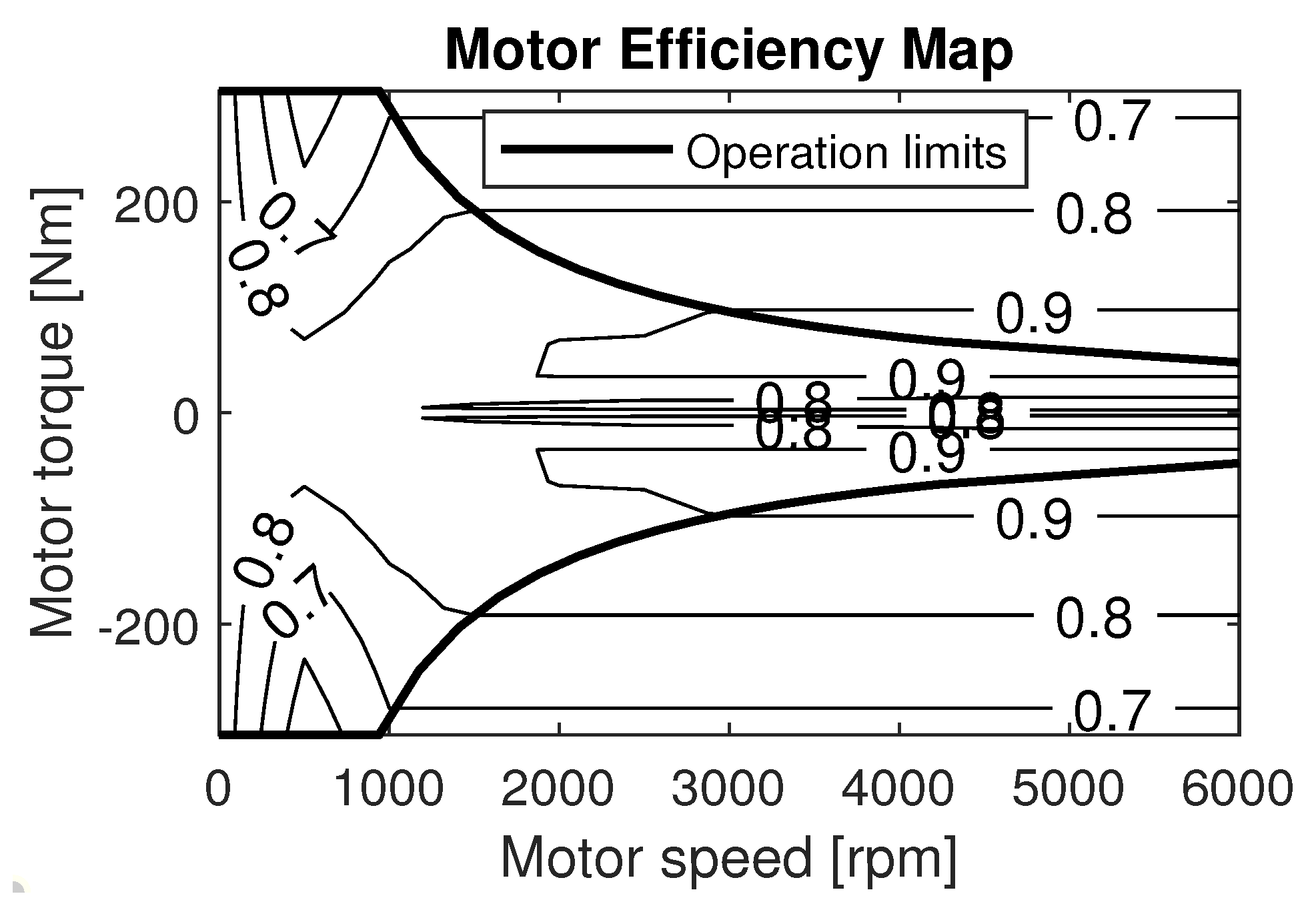
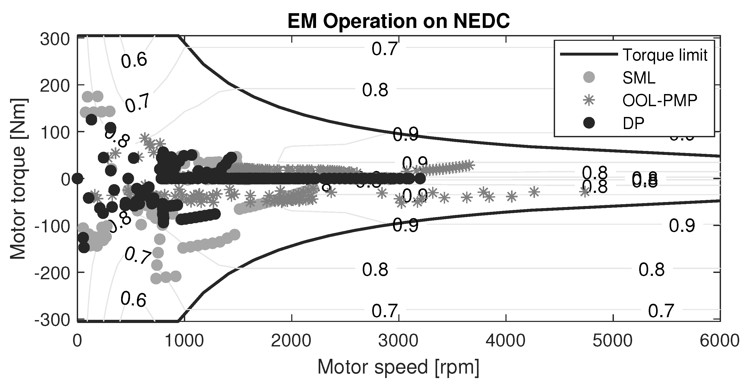
Electric motor: The 30-kW permanent magnet EM is taken from the 1999 Toyota Prius PHEV (Aichi, Japan). The efficiency of the EM (
) can be determined from the efficiency map in
Figure 5 and the output power of the battery (
) can be calculated as in Equation (
14). The data for the efficiency map are taken from test bench measurements [
41]:
Battery: The 288-V and 6-Ah nickel metal hydride (NiMH) battery pack is taken from the Toyota Prius 2000 model. It is modeled as a voltage input with an internal resistance for simulation and as an equivalent resistance circuit to achieve convexity in the Hamiltonian. The test bench measurements from the Insight battery pack are scaled up to the Prius battery pack [
42]. The coulombic efficiency (
) is assumed to be 0.905 for charging and discharging. The current within the battery can be calculated from the output power of the battery, and is given in Equation (
15):
Subsequently,
where
is the battery current,
is the open circuit voltage, Ω is the internal resistance of the battery circuit,
is the power output of the battery,
is the coulombic efficiency of the battery,
is the state of charge,
t is the time instance, and
is the nominal battery capacity.
With the system modelled, the next section describes the formulation and solution of the control problem.
3. Methodology
In this section, the control problem is formulated in
Section 3.1. Subsequently, the solution for this control problem using the proposed SML framework is described in
Section 3.2. In order to evaluate the performance of the proposed SML framework, conventional solutions such as DP is elaborated upon in
Section 3.3 and an online implementable control strategy OOL-PMP is introduced and described in
Section 3.3.
3.1. Control Problem
The objective of the control problem is to minimize energy consumption over the drive cycle, while satisfying the physical constraints of the system. Considering the practical application of a PHEV, the boundary conditions for state of charge (
,
) is fixed for a given drive cycle and the fuel consumption (
) is minimized:
where
is the initial time and
is the final time.
The control problem can be formulated as:
State space; x = {} where with of battery capacity) and of battery capacity). Control space; u = {, } where and with and . is the costate that satisfies the boundary conditions for PMP.
The following subsection introduces the machine learning framework that is proposed as a solution for the control problem.
3.2. Solution Using Supervised Machine Learning
A few comments are in order, and it is assumed that a robust baseline strategy exists while training data are being accumulated. Secondly, in order to satisfy the objective (), the controller training is performed from scratch. Thirdly, in the specified framework, training occurs on completion of the driving task. Therefore, it is assumed that the vehicle is equipped with sufficient memory to store vehicle states.
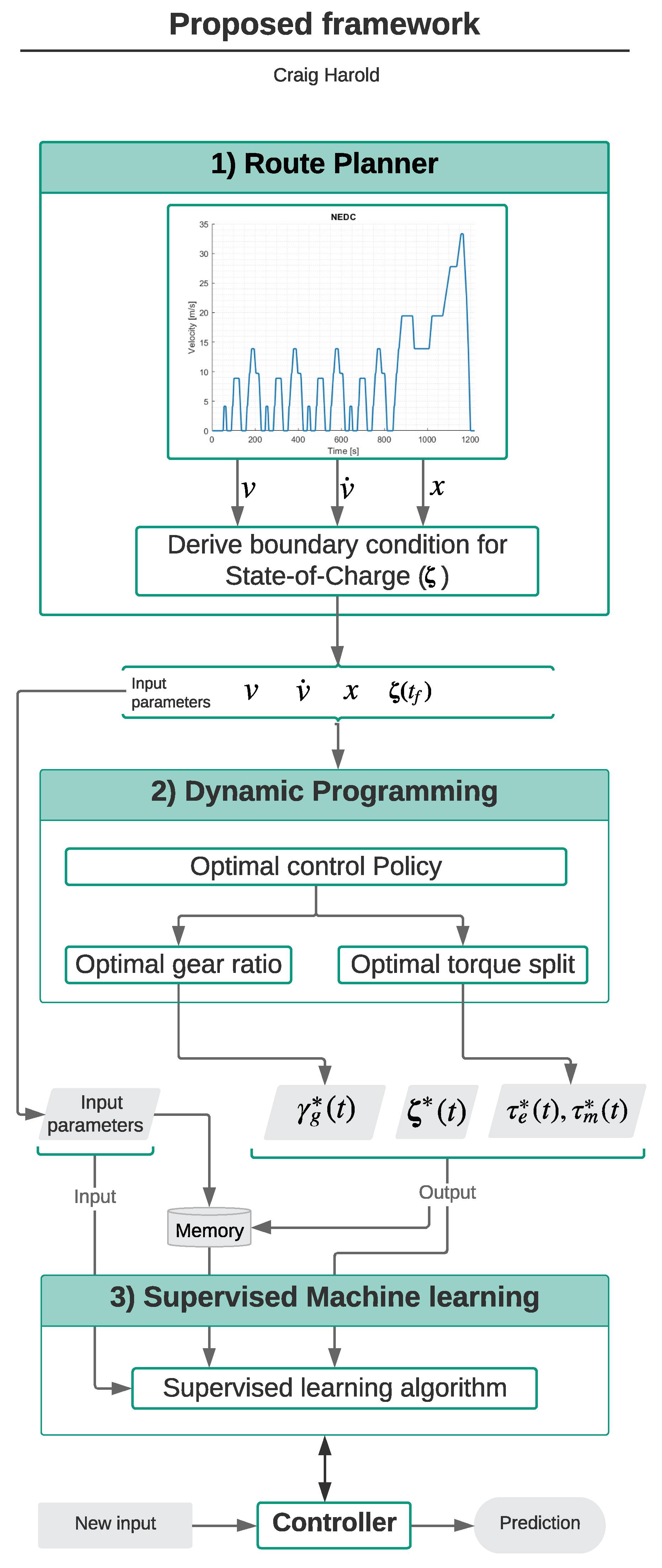
Proposed Framework: The framework is divided into three segments, namely, Route Planner (RP), Dynamic Programming (DP), and Supervised Machine Learning (SML). The flow of events and parameters are illustrated in
Figure 6:
Route Planner records the drive cycle and the initial condition (
) for the respective drive cycle. The velocity trajectory depicted in the route planner segment in
Figure 6 is an example of the recorded drive cycle. Based on this drive cycle, an end-point condition
is determined. In this study,
is calculated assuming 1.1% battery charge is available for the distance of 1 km. The assumption is made based on the average driving and charging cycles of HEVs in the Netherlands [
43]. The requirement of the route planner is to set the boundary condition for the a priori drive cycle. There are more sophisticated planners based on traffic congestion, terrain, charging stations, etc. but do not add value to this study, hence neglected.
Secondly,
Dynamic Programming solves the two-point boundary value problem satisfying
resulting in the optimal control policy (
,
) and optimal state trajectory (
,
), for the given drive cycle. The discretized state and control spaces are elaborated in
Section 3.3.
Thirdly,
Supervised Machine Learning segment develops a control strategy by mapping the input parameters from the drive cycle to the optimal control policy from DP, using SML algorithms. The rules derived from this mapping represent the control strategy and make predictions for a new input as shown in
Figure 6. No universal algorithm exists to model the system; therefore, an SML algorithm is selected based on an exhaustive search. The SML algorithm is selected with a five-fold cross validation based on its accuracy of predictions, deviation of false predictions from the optimal value, and computational time for each prediction. The various algorithms are shown in
Table 1 along with their prediction accuracy and the number of predictions the algorithm is capable of every second. Both characteristics are desired to be as high as possible and based on this, the selected algorithm is highlighted. Additionally, a memory module is used to store previously recorded data for the purpose of re-training the controller.
The learning algorithms used for individual control strategies are discussed in
Section 3.2.1 and the parameters with which the algorithm achieved the accuracy and prediction speed highlighted in
Table 1 are introduced.
3.2.1. Supervised Machine Learning Algorithms
Decision Tree: As the name suggests, decision tree (DT) builds a model for the data to go from observation to prediction through branches. It is representative of a root system beneath a tree and is also representative of human decision-making. Each node represents binary logic and filters down to a prediction based on this set of binary logic gates. The nodes of the tree are split based on impurity gain (
), given by Equation (
18):
where
is the probability of the splitting candidate or node
t in the set of all observations
T,
is the probability that left child node (
) is present in the left observation set
and
is the probability that the right child node (
) is present in the right observation set (
. In essence, a node is selected and all the observations are partitioned at the node. The impurity gain checks the number of instances of a class that are common on both sides of the partition, thereby the impurity of the class.
For this study, the primary pulley speed (
), the torque demand at the primary pulley (
), and the state of charge of the battery (
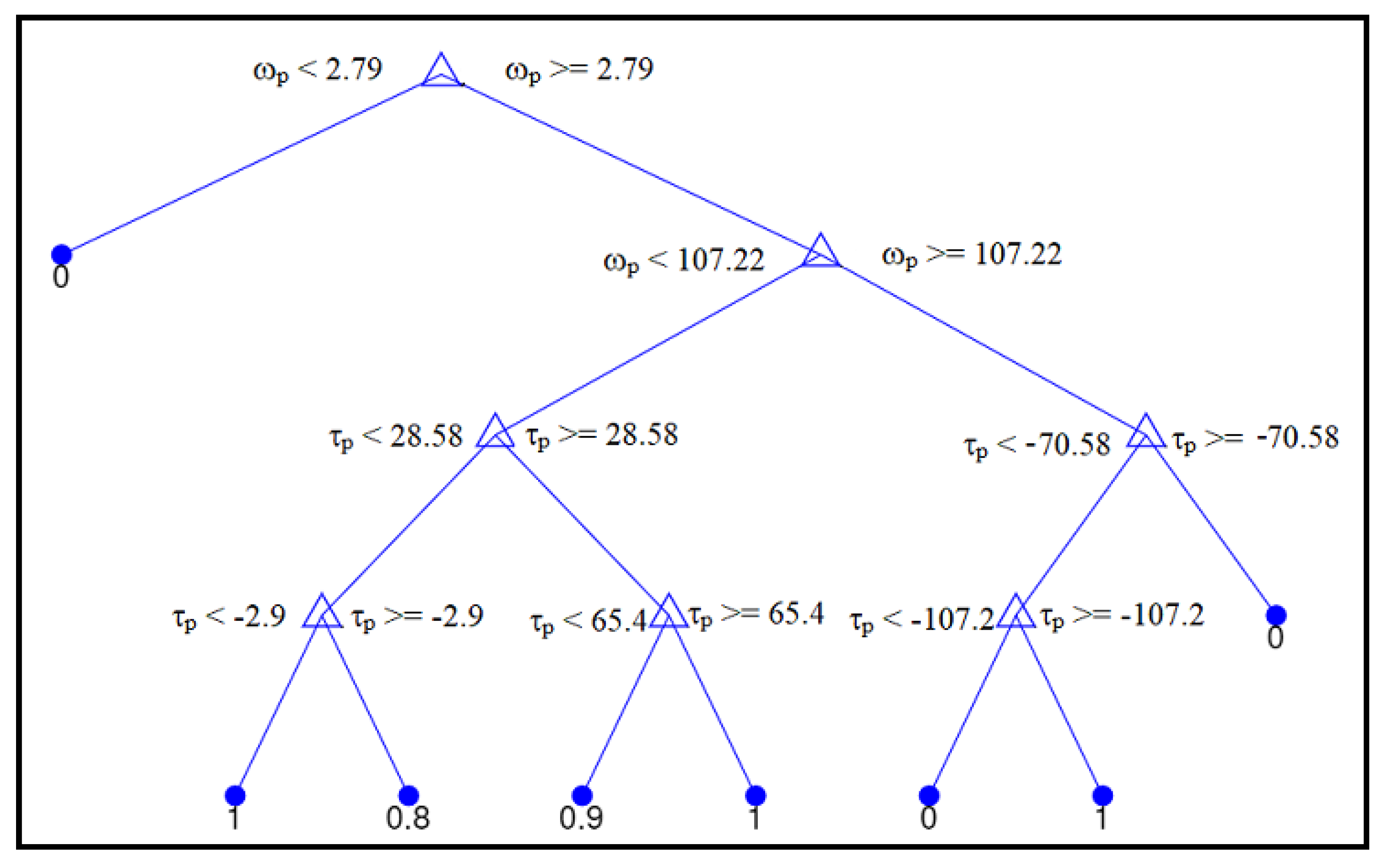
) were used as input features, and the optimal torque split was the desired output from the DT. The properties of the decision tree used for training are as follows: maximum number of splits was set to 100 and k-fold cross validation is set to 5. An example with relevance to the system model is depicted in
Figure 7, wherein the decision tree is trained for torque split control, but limited to 10 nodes. It is intuitive that, for the negative torque demand (power flow from the wheels to the energy source), the resulting torque split is closer to 1 indicating complete regeneration.
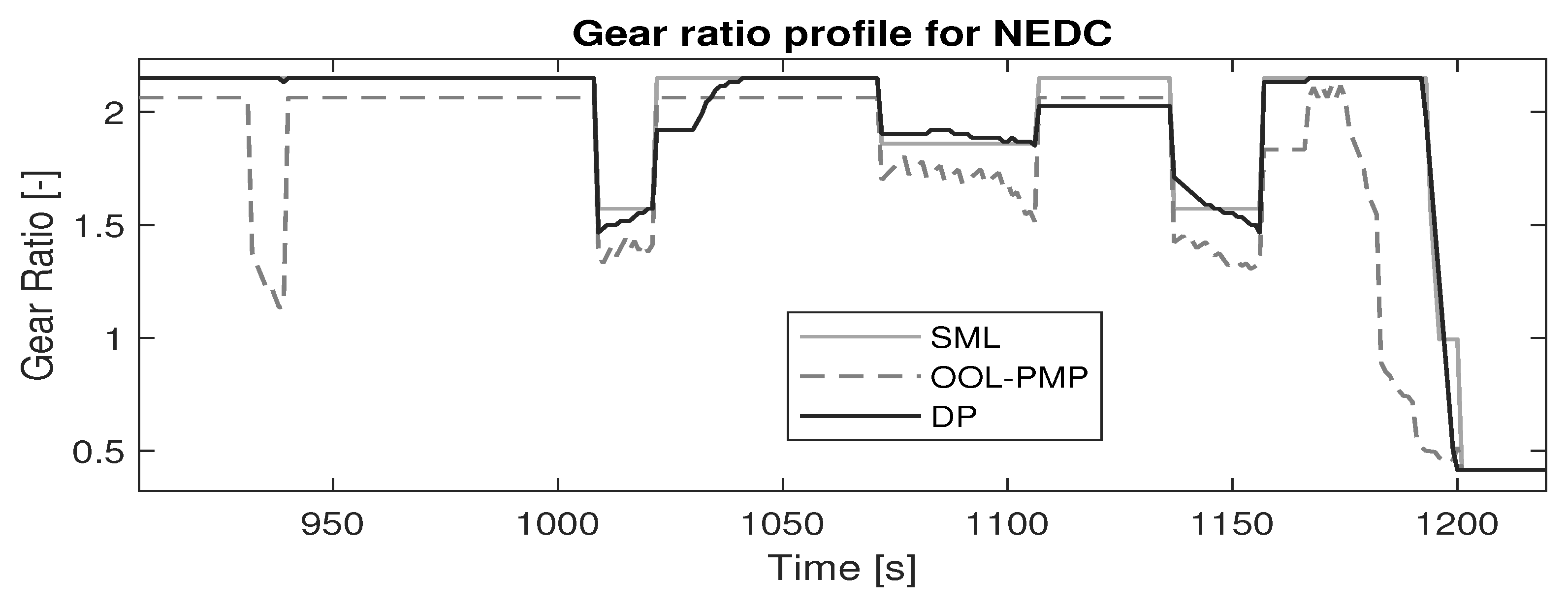
K-Nearest Neighbors: The K-Nearest Neighbor (KNN) algorithm is non-parametric, i.e., no model is fitted to the data and all the work is done when a prediction is required. In principle, the KNN algorithm takes a vote of the closest neighbors to predict an output. The ‘K’ in KNN represents the number of neighbors to consider. Therefore, the ‘K’ should be an odd number to ensure a majority in the vote. KNN is used as the gear ratio control algorithm, wherein the input features are the vehicle speed (v) and vehicle acceleration () and the desired output is the optimal gear ratio (). It must be noted that is used as a feature since the drivecycles considered do not include elevation profiles. In case of non-horizontal drivecycles, the torque required at the secondary pulley () will substitute and in case of a forward facing model or practical applications, the throttle input will substitute . The properties of the KNN algorithm used are as follows; the closest neighbors are determined by the Euclidean distance, the number of votes accounted for is 7, equal weighting given to all neighbors and the k-fold cross validation is set to 5. It must be noted that to ensure effective learning with the limited available data points from each drive cycle, the CVT was discretized into seven equally spaced classes for the SML case—ergo limiting the performance of the SML control strategy. However, with the abundance of data from real-world driving, this limitation can be overcome and in turn the full potential of the CVT can be exploited.
In order to evaluate the performance of the proposed framework, the SML controller is compared to conventional solutions that are elaborated in
Section 3.3.
3.3. Solutions Using Classical Control
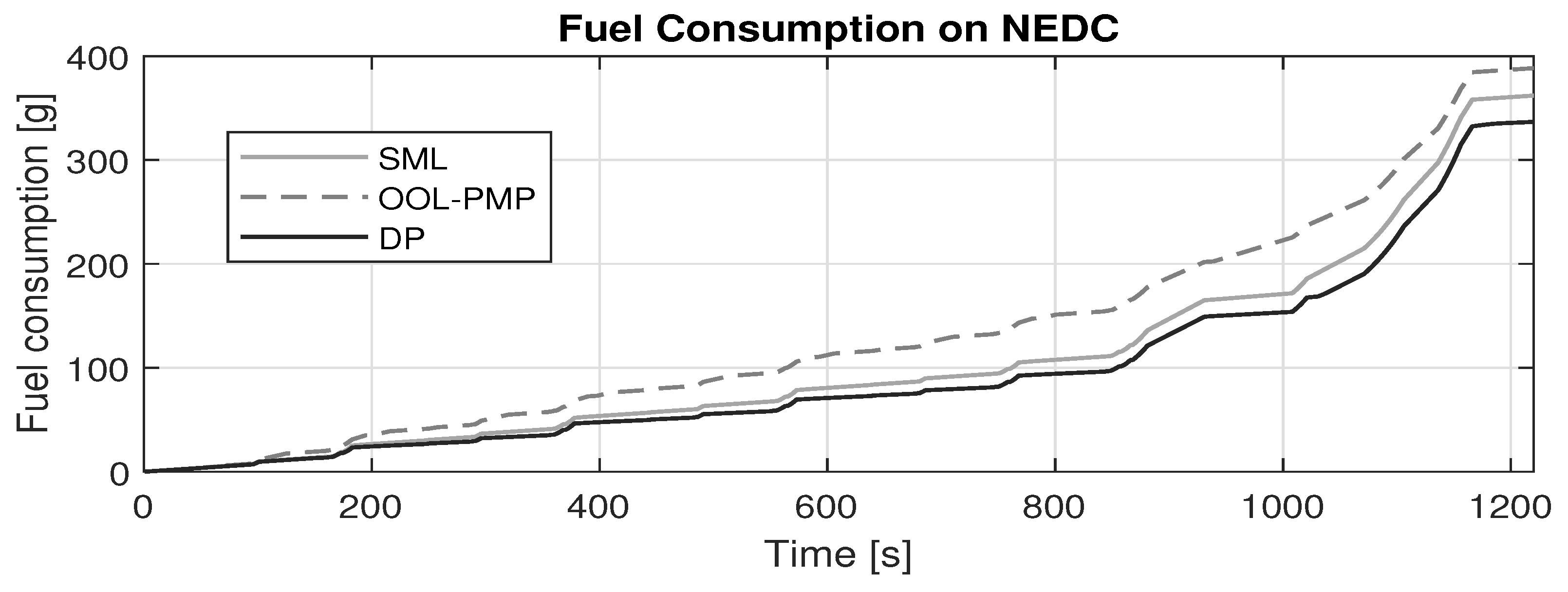
To validate the SML controller, its performance is compared to the global benchmark set by DP and the online implementable benchmark set by OOL-PMP.
Global Benchmark, DP: DP results in the global optimal control policy for the a priori drive cycle with boundary conditions and . A cost matrix is built with all possible state-action combinations at each timestep through the drive cycle. All infeasible states or actions are penalized with a high cost. Finding a path with minimal cost through the cost matrix results in the optimal control policy.
In order to build the cost matrix, the state and control space is discretized. The CVT is discretized into 100 gear ratios to exploit the full potential of the CVT. The torque split control (
) is discretized into intervals of 0.05, and the implication of the torque split variable is shown in Equations (
19) and (
20). For cases where
,
where
is the rotational speed of the primary pulley and
is the torque required at the primary pulley. The state space
is discretized as follows:
in intervals of 0.005 and
discretized to 100 ratios. The time interval of 1 s is chosen since the difference in
is very small for any smaller intervals of time.
Online Benchmark, OOL-PMP: The combination of OOL-PMP is based on a decoupled approach from the literature review in
Section 1.1. The OOL is constructed by using the most efficient points of ICE operation over the entire ICE speed range and is used to control the gear ratio (
), while the PMP method is used to control the torque split (
). Since the system is modeled as backward facing, the power required at the primary pulley (
) is estimated and subsequently a gear ratio is selected by OOL. It is counter-intuitive to use a torque split controller in combination with OOL, since OOL inherently determines the operating point of the ICE and ergo the operating point of the EM based on the power request at the primary pulley. However, to ensure that the torque split is optimal and online-implementable, a PMP approach is used to control the torque split. The formulation of the Hamiltonian and application of PMP is taken from [
22] and given in Equation (
21). The losses in the EM are modelled as a second degree polynomial, while the ICE losses and BAT open-circuit voltage are approximated by a linear fit. The control variable chosen is the power of the battery (
):
where
is the fuel power, x is the state of charge (
),
is the time derivative of
, and (
p) is the costate:
where
is the power required at the primary pulley of the CVT, (
,
) are the coefficients of the linear fit that models the ICE losses, (
,
,
) are the coefficients of the second degree polynomial used to model the EM losses,
is the open-circuit voltage of the BAT, and
is the resistance of the BAT.
The necessary conditions of PMP are as follows:
Solving the first condition results in the optimal
, shown in Equation (
23):
Solving this as an initial value problem using a bisection algorithm results in the initial costate that satisfies the boundary conditions and . In order to the solve this boundary value problem, the exact velocity and acceleration profile from the respective drivecycle are considered.
With the proposed SML solution described along with the conventional solutions in order to compare the performance of the SML control strategy, the following
Section 4 discusses the results of the study.
5. Conclusions
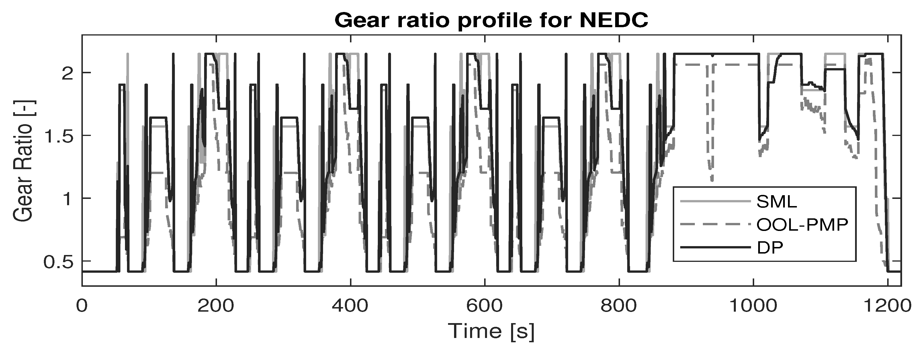
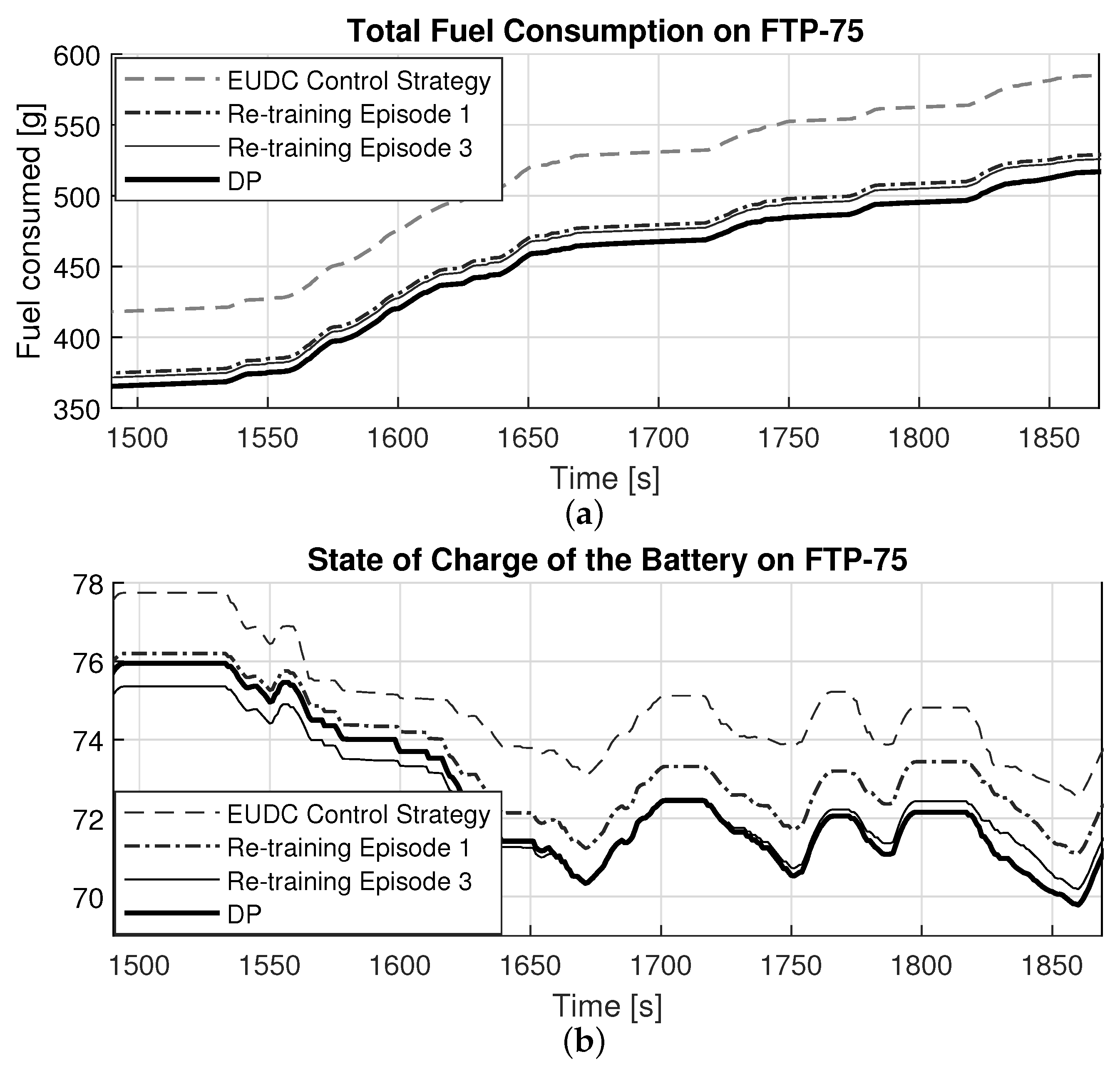
The results show that the learned control strategy (SML) outperforms the conventional online implementable strategy (OOL-PMP), tested over several standard drivecycles in terms of fuel economy. This indicates that the proposed framework could effectively learn from past driving experiences to reproduce close to optimal results for the identical training conditions, i.e., the same drivecycle. However, since real-world driving will seldom experience identical training conditions, it is critical to study the efficacy of the proposed framework in adapting the control strategy to newly experienced drivecycles. Therefore, a test-case is conducted wherein the control strategy trained for EUDC is utilized on the FTP-75 and the effect of re-training the control strategy with the new drivecycle is observed. The EUDC strategy applied to the FTP-75 showed a large deviation from the optimal trajectory and a single episode of re-training significantly bridged the gap to optimality. Therefore, the proposed framework could be a viable alternative to the existing control strategies that adapts efficiently to a specific driver behavior.
Downsides of this proposed framework are briefly highlighted, the requirement of on-board computational power to perform DP is a real-world limitation but off-loading the computational burden is a prospective solution, since modern cars already record vehicle data and upload it to a cloud in the presence of internet connectivity. Furthermore, the algorithm properties, size of the dataset, and quality of dataset have shown to affect the performance and require more in-depth research.
As for future applications and improvements, the current framework using past data can be replaced with a predicted drive cycle based on geographic location, traffic congestion, terrain, weather, etc. that is easily available with current map technology. Additional states can be added, such as a slope sensor to consider the elevation of the road, in turn providing a more extensive control strategy capable of accounting for dynamic environments.


