1. Introduction
Open science, including open data, has been marked as the future of science [
1], and the advantages of publicly available research data are numerous [
2,
3]. Collecting research data requires an enormous investment both in terms of time and monetary resources. Disseminating the research data increases the potential scientific returns for the same data collection effort tremendously. Additionally, the fact that public funds are used for data collection results in increasing demand for access to the collected data. Nevertheless, the possibilities for distribution of research data directly are often very limited due to restrictions of data privacy and data confidentiality. Although these regulations are much needed, privacy constraints are also ranked among the toughest challenges to overcome in the advancement of modern social science research [
4].
Anonymizing research data might seem a quick and appealing approach to limit the unique identification of participants. However, this approach is not sufficient to fulfill contemporary privacy and confidentiality requirements [
5,
6]. Over the years, several other techniques have been used to increase the confidentiality of research data, such as categorizing continuous variables, top coding values above an upper bound, or adding random noise to the observed values [
7]. However, these methods may distort the true data relation between variables, thereby reducing the data quality and the scientific returns for re-using the same data for further research.
An alternative solution has been proposed separately by Rubin [
8] and Little [
9]. Although their approaches differ to some extent, the overarching procedure is to use bonafide observed data to generate multiply imputed synthetic datasets that can be freely disclosed. While in practice, one could see this as replacing the observed data values by multiple draws from the predictive distribution of the observed data, based on some imputation model, Rubin would argue that these synthetic data values are merely drawn from the same true data generating model. In that sense, the observed data are never replaced, but the population is resampled from the information captured in the (incomplete) sample. Using this approach, the researcher could replace the observed dataset as a whole with multiple synthetic versions. Alternatively, the researcher could opt to only replace a subset of the observed data. For example, one can choose to only replace dimensions in the data that could be compared with publicly available datasets or registers. Likewise, synthesization could be limited to those values that are disclosive, such as high incomes or high turnovers.
Conceptually, the synthetic data framework is based upon the building blocks of multiple imputation of missing data, as proposed by Rubin [
10]. Instead of replacing just the missing values, one could easily replace any observed sensitive values by multiple draws from the posterior predictive distribution or a non-Bayesian predictive distribution (both of these will be referred to as predictive distributions throughout). Similar to multiple imputation of missing data, the multiple synthetic datasets allow for correct statistical inferences, despite the fact that the analyses do not use the
true value. The analyses over multiple synthetic datasets should be pooled into a single inference, so that the researcher can draw valid conclusions from the pooled results. In that respect, the variance should reflect the added variability that is induced by the imputation procedure.
Potentially, this approach could fulfill the needs for openly accessible data, without running into barriers with regard to privacy and confidentiality constraints. However, there is no such thing as a free lunch: data collectors have to put effort in creating high-quality synthetic data. The quality of the synthetic data is highly dependent on the imputation models, and using flawed imputation models might bias subsequent analyses [
11,
12,
13]. Conversely, if the models used to synthesize the data are able to preserve the relationships between the variables as in the original data, the synthetic data can be nearly as informative as the observed data. To fully exploit the benefits of synthetic data, complicating aspects of creating high-quality synthetic datasets should be kept at a minimum, while keeping the accuracy of the models as high as possible.
To mitigate unnecessary challenges related to creating synthetic data sets on behalf of the researcher, software aimed at multiple imputation of missing data can be employed. In particular, if researchers acquired familiarity with this software during earlier projects, or used it earlier in the research process, the additional burden of creating synthetic datasets is relatively small. The R-package
mice [
14] implements multiple imputation of missing data in a straightforward and user-friendly manner. However, the functionality of
mice is not restricted to the imputation of missing data, but allows imputation of any value in the data, even observed values. Consequently,
mice can be used for the creation of multiply imputed synthetic data sets.
After creating multiply imputed synthetic datasets, the goal is to obtain valid statistical inferences in the spirit of Rubin [
10] and Neyman [
15]. In the missing data framework, this is done by performing statistical analyses on all imputed datasets, and pooling the results of the analyses according to Rubin’s rules ([
10], p. 76). In the synthetic data framework, the same procedure is followed, but with a slight twist; there may be no values that remain constant over the synthetic datasets. The procedure of drawing valid inferences from multiple synthetic data sets is therefore slightly different.
In this manuscript, we detail a workflow for synthesizing data with mice. First, the mice algorithm for the creation of synthetic data will be briefly explained. The aim is to generate synthetic sets that reassure the privacy and confidentiality of the participants. Second, a straightforward workflow for imputation of synthetic data with mice will be demonstrated. Third, we demonstrate the validity of the procedure through statistical simulation.
2. Generating Synthetic Data with
mice
Generally, there are three ways to impute data: joint modeling, sequential modeling, and fully conditional specification [
12,
16,
17]. With joint modeling, the entire joint distribution of the data is specified as a single multivariate distribution, and the imputations are drawn from this model. This strategy is implemented in, among others, the
R-package
jomo [
18] to deal with missing data. However, when the structure of the data increases in complexity, specifying a single multivariate distribution that would fit the observed data can become challenging. A more flexible solution has been proposed in sequential regression imputation, in which the multivariate distribution is separated into univariate conditional distributions. Every single variable is then imputed conditionally on a model containing only the variables in the sequence located before the variable to be imputed. This approach has been implemented in the R-packages
mdmb [
19] for imputation of missing data and
synthpop [
20] for imputation of synthetic data.
Fully conditional specification (FCS) has been implemented in the
mice package [
14,
21] in
R [
22], which has been developed for multiple imputation to overcome problems related to nonresponse. In that context, the aim is to replace missing values with plausible values from the predictive distribution of that variable. This is achieved by breaking down the multivariate distribution of the data
into
univariate conditional densities, where
k denotes the number of columns in the data. Using FCS, a model is constructed for every incomplete variable and the missing values
are then imputed with draws from the predictive distribution of
on a variable-by-variable basis. Note that the predictor matrix
may contain yet imputed values from an earlier imputation step, and thus will be updated after every iteration. This procedure is applied
m times, resulting in
m completed datasets
, with
.
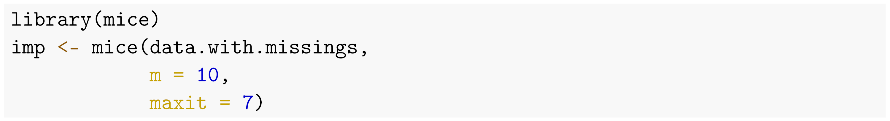
In mice (Version 3.13.15), the generation of multiply imputed datasets to solve for unobserved values is straightforward. The following pseudocode details multiple imputation of any dataset that contains missingness into the object imp with m = 10 imputated sets and maxit = 7 iterations for the algorithm to converge, using the default imputations methods.
![Psych 03 00045 i001]()
The imputation approach in
mice can be easily extended to generate synthetic values. Rather than imputing missing data, observed values are then replaced by synthetic draws from the predictive distribution. For simplicity, assume that the data are completely observed (i.e.,
). Following the notation of Reiter and Raghunathan [
23], let, given
n observations,
if any of the values of unit
, are to be replaced by imputations, and
otherwise, with
. Accordingly, the data consist of values that are to be replaced and values that are to be kept (i.e.,
. Now, instead of imputing
with draws from the predictive distribution of
as in the missing data case,
is imputed from the posterior distribution of
, where
l is an indicator for the synthetic dataset (
). This process results in the synthetic data
.
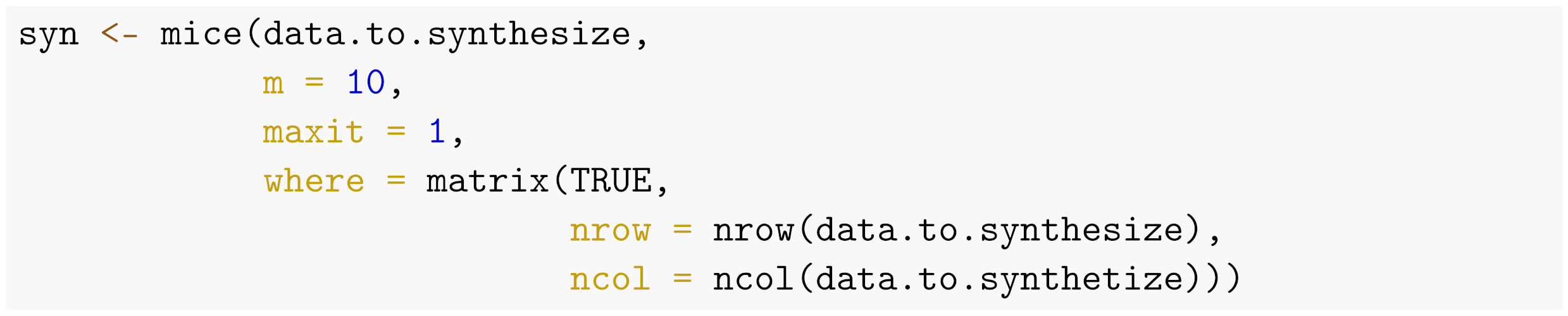
Hence, creating synthetic values for a completely observed dataset into the object syn, given the same imputation parameters as specified above, can be realized as follows:
Here, the argument where requires a matrix of the same dimensions as the data, (i.e., a matrix) containing logicals that indicate which cells are selected to have their values replaced by draws from the predictive distribution. This approach enables replacing a subset of the observed data (e.g., by specifying only those cells that are to be replaced as TRUE in the where-matrix, leaving the rest to FALSE), or as in the aforementioned example, the observed data as a whole, resulting in a dataset that partially or completely consists of synthetic data values. Note that because the data are completely observed, iterating over the predictive distribution is not required.
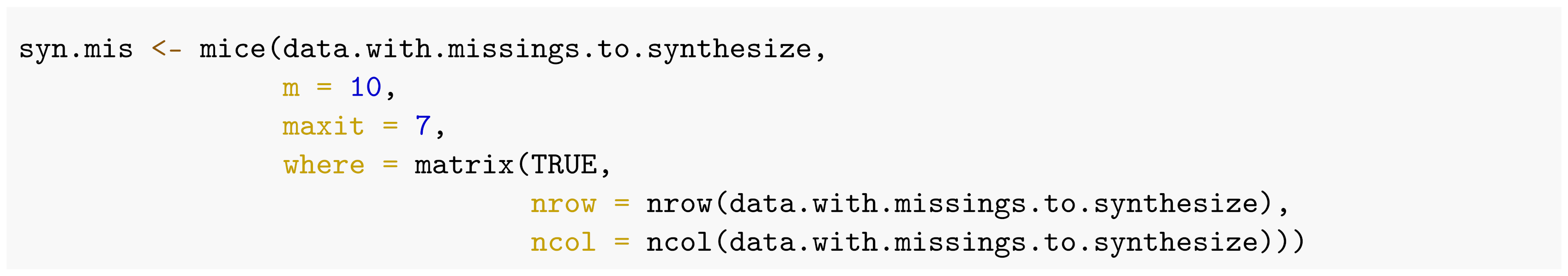
If the goal is to create synthetic versions of a dataset that suffers from missingness, the imputation procedure becomes more complex. A two-step imputation procedure has been proposed by Reiter [
11]. In the first step, the missing data are imputed according to the principles of multiple imputation for missing data, while in a second step, the synthetic data are imputed to conform the corresponding procedure. Ideally, these steps could be combined using
mice, conditioning the imputations on both the missingness and the values that are to be synthesized. In practice, replacing observed and missing cells in a dataset by synthetic values into the object
syn.mis, given the same imputation parameters as before, can be realized by the following code execution.
However, because the validity of this approach when the data suffer from missingness has not been investigated yet, we restrict ourselves in the following sections to a completely observed data set.
Choosing an adequate imputation model to impute the data is paramount, as a flawed imputation model may drastically impact the validity of inferences [
12,
13]. Imputation models should be as flexible as possible to capture most of the patterns in the data, and to model possibly unanticipated data characteristics [
16,
24]. Generally, multiple methods can be feasible, including joint modeling, sequential regression and FCS, all with different parameter specifications, depending on the imputation problem at hand [
17,
25,
26]. Various simulations have shown that the most accurate imputation procedure may vary over different imputation problems (e.g., see [
27] for an overview). Hence, a one-size-fits-all solution does probably not exist.
However, one of the methods that has shown a reasonable and consistent performance over multiple simulations (e.g., [
28,
29,
30,
31]) is FCS in combination with classification and regression trees (CART; [
32]). Due to its nonparametric nature, CART enables modeling complex patterns (e.g., interactions and nonlinear relationships) in the data. Loosely speaking, CART sequentially splits the predictor space into non-overlapping regions in such a way that the within-region variance is as small as possible after every split. As such, CART does not impose any parametric distribution on the data, making it a widely applicable method that allows for a large variety of relationships within the data to be modeled [
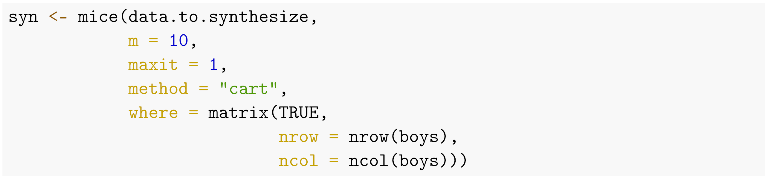
33]. Given these appealing characteristics and the call for the use of flexible methods when multiply imputing data, we will focus our illustrations and evaluations of
mice to method
mice.impute.cart(), realized by:
![Psych 03 00045 i004]()
In a nutshell, the above code shows the simplicity of creating
synthetic datasets using
mice. In practice, however, one should take some additional complicating factors into account. For example, one should account for deterministic relations in the data. Additionally, relations between variables may be described best using a different model than
CART. Such factors are data dependent and should be considered by the imputer. In the next section, we will describe how a completely observed version of the
mice::boys data [
34] can be adequately synthesized. Additionally, we will show through simulations that this approach yields valid inferences.
4. Results
The synthetic data are evaluated with respect to the true dataset on the basis of three aims. We believe that every reliable and valid data synthesization effort in statistical data analysis should be able to yield (1) unbiased univariate statistical properties, (2) unbiased bivariate properties, (3) unbiased and valid multivariate inferences, and (4) synthetic data that cannot be distinguished from real data. We consider the evaluation of the synthetic data simulations in the above order.
4.1. Univariate Estimates
The univariate descriptives for the original data and the synthetic data can be found in
Table 2. From this table, it can be seen that the synthetic data estimates closely resemble the true data estimates. All sample statistics of interest show negligible bias over the 1000 synthetic data sets.
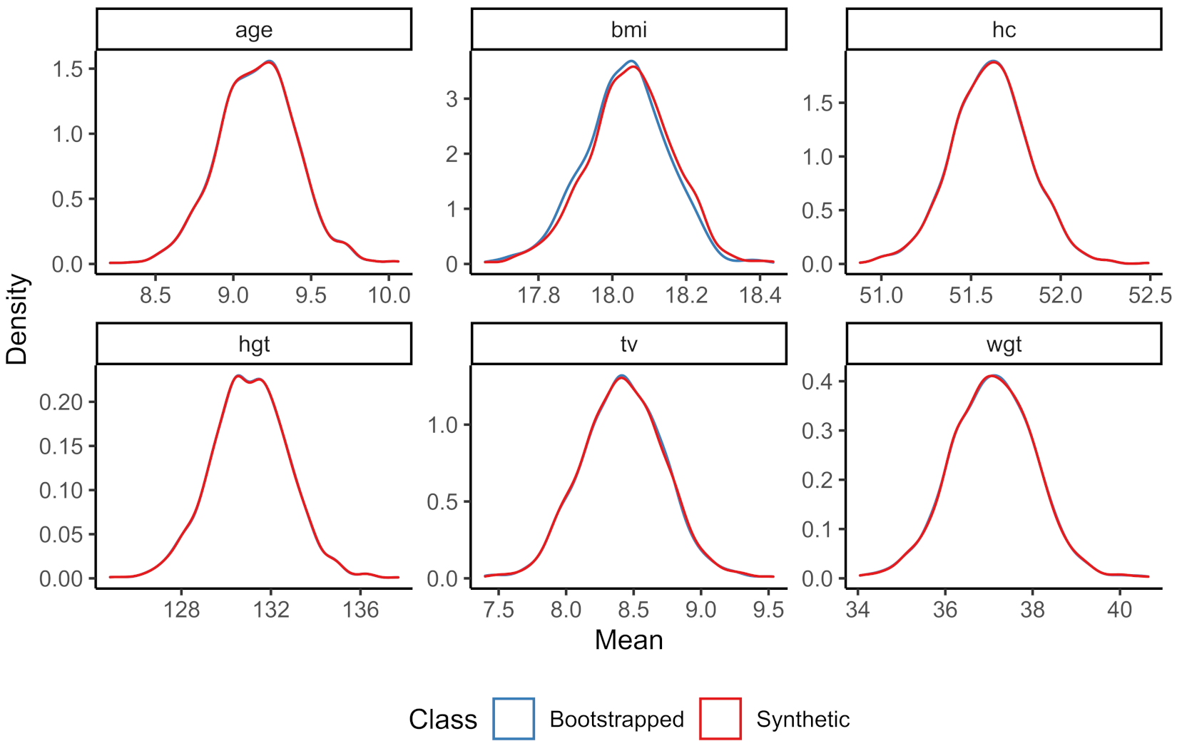
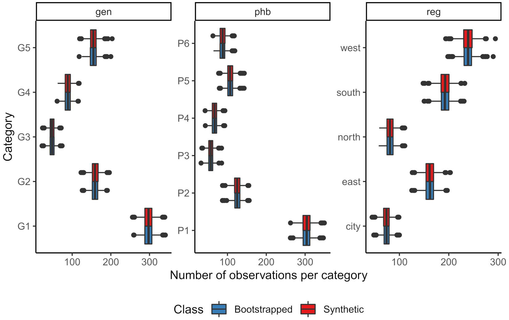
The sampling distribution of the means of the continuous variables for both the bootstrapped and the synthetic data can be found in
Figure 1, while the number of observations per category in the bootstrapped data and the averaged number of observations per category over the synthetic datasets can be found in
Figure 2.
Both figures show that the marginal distributions of the bootstrapped data and the synthetic data are highly similar. The sampling distributions of these parameters hardly seem to differ. Hence, both the numeric and graphical results show that univariately the synthesis model proves adequate.
4.2. Bivariate Estimates
An often used bivariate statistic is Pearson’s correlation coefficient. When evaluating this correlation coefficient on the numeric columns in the
boys dataset, the differences between the correlations in the synthetic and bootstrapped data are very small. These results are displayed in
Table 3.
The correlations obtained from synthetic data are unbiased with respect to the true dataset. The largest bias over 1000 simulations equals 0.013, indicating that the imputation model is capable of preserving the bivariate relations in the data.
4.3. Multivariate Model Inferences
First, we evaluate the performance of our synthetic simulation set on a linear model where
hgt is modeled by a continuous predictor
age and an ordered categorical predictor
phb. The results for this simulation can be found in
Table 4.
We see that the finite nature of the true dataset together with the design-based simulation setup yields slight undercoverage for the terms of phb. This finding is observed in both the bootstrap coverages (i.e., the fraction of 95% confidence intervals that cover the true data parameters) and the synthetic data coverages. Hence, it is likely that this undercoverage stems from the simulation setup, rather than the imputation procedure. Besides the undercoverage, there is a tiny bit of bias in the estimated coefficients of the variable phb that occurs in the synthetic estimates, but not in the observed estimates. Yet, since the bias is relatively small and does not result in confidence invalidity, it seems fair to assume that the introduced bias is not that problematic.
Second, we evaluate a proportional odds logistic regression model in which the ordered categorical variable
gen is modeled by continuous predictors
age and
hc, and the categorical predictor
reg. The results for this model are shown in
Table 5.
These results demonstrate that the synthetic data analysis yields inferences that are on par with inferences from the analyses directly on the bootstrapped datasets. Hence, for the regression coefficients as well as the intercepts, the analyses on the synthetic data yield valid results. Nevertheless, a small amount of bias is introduced in the estimated intercepts of the synthetic data. However, the corresponding confidence interval coverage rates are actually somewhat higher than the confidence interval coverage rates of the bootstrapped data. Therefore, the corresponding inferences do not seem to be affected by this small bias.
4.4. Data Discrimination
When we combine the original and synthetic data, can we predict which rows come from the synthetic dataset? If so, then our synthetic data procedure would be redundant, since the synthetic set differs from the observed set. To evaluate whether we can distinguish between the true data and the synthetic data, we combine the rows from each simulation synthetic dataset with the rows from the true data. We then run a logistic regression model to predict group membership: i.e., does a row belong to the true data or synthetic data. As predictors we take all columns in the data. The pooled parameter estimates over all simulations can be found in
Table 6.
From these pooled results we can see that the effects for all predictors are close to zero and nonsignificant. When we take the predicted values from the simulated models and compare them with the
real values, we obtain the summary statistics in
Table 7.
The accuracy of the predictive modeling effort is not better than random selection, and the Kappa coefficient indicates that a perfect prediction model is far from realized. The accuracy is quite balanced as there is no skewness over sensitivity and specificity. These findings indicate that the synthetic data are indistinguishable from the true data.
5. Discussion
We demonstrated that generating synthetic datasets with
mice using CART in
R is a straightforward process that fits well in a data analysis pipeline. The approach is hardly different from using multiple imputation to solve problems related to missing data and, hence, can be expected to be familiar to applied researchers. The multiple synthetic sets yield valid inferences on the true underlying data generating mechanism, thereby capturing the nature of the original data. This makes the multiple synthetisation procedure with
mice suitable for further dissemination of synthetic datasets. It is important to note that in our simulations we used a single iteration and relied on CART as the imputation method. A single iteration is sufficient only when the true data are completely observed, or when the missingness pattern is monotone [
7]. If both observed and unobserved values are to be synthesized, then more iterations and a careful investigation into the convergence of the algorithm are in order. Synthetic data generation is therein no different than multiple imputation.
When creating synthetic data with
mice, close attention should be paid to three distinct factors: (i) the additional uncertainty that is due to synthesizing (part of) the data should be incorporated, (ii) potential disclosure risks that remain after synthesizing the data should be assessed, and (iii) the utility of the synthetic data should be examined. First, the procedure of generating multiple synthetic sets may seem overly complicated. We would like to emphasize that analyzing a single synthesized set, while perhaps unbiased, would underestimate the variance properties that are so important in drawing statistical inferences from finite datasets. After all, we are often not interested in the sample at hand, but aim to make inferences about the underlying data generating mechanism as reflected in the population. Properly capturing the uncertainty of synthetic datasets, just like with incomplete datasets, is therefore paramount. To achieve this, we adopted a bootstrap scheme in our simulations, to represent sampling from a superpopulation. However, when a single sample should be the reference, in the sense that the sample reflects the population one wishes to make inferences about, adjusted pooling rules are required that are similar to the procedure outlined in Vink and van Buuren [
37]. The corresponding pooling rules have not been derived yet and the incorporation in data analysis workflows would require proper attention from developers alike.
Second, it is important that imputers pay close attention to disclosure risks that remain after creating synthetic datasets. Creating synthetic data, unless generated from a completely parametric distribution, does not remove all potential disclosure risks. For example, if the values that ought to be replaced have the exact same value imputed, the synthesization procedure has no use. Additionally, if not all variables in the data are synthesized, but the variables that are synthesized can be linked to open access data, a disclosure risk may remain [
38]. If the open access data allow for identification, and the corresponding observations in the synthetic data can be identified, the variables that are not synthesized may provide information that should not have been disseminated. The associated problems generally decrease when the sensitive variables are synthesized as well. Still, it is important to remain critical regarding the extent to which the synthetic data might be disclosive. The practical development of easy-to-use software to identify which observations are at risk of disclosure is an area of future work that can improve these issues. Subsequently, the implementation of ways to overcome such problems once detected, for example by record swapping as suggested by Jiang et al. [
13], is welcomed.
Third, the utility of the synthetic data should receive considerable scrutiny. After all, synthetic data are generated to allow third parties without access to the data to draw valid inferences. If the quality of the synthetic data is very poor, the validity of inferences is at stake. We showed that CART proved to be an adequate method for the data at hand. However, it may well be that for some problems, using CART for imputation is not the optimal strategy. We already demonstrated that imputing deterministic relationships should not be based on CART. However, due to the variety in possible imputation methods that have proved to perform well in varying circumstances, providing a single solution to all synthesis problems seems impossible. If required, imputers could build up their synthesis models in complexity. Nevertheless, similar to past research (e.g., [
29,
30,
31]), we showed that CART provides adequate results in general, and therefore serves as a good starting point.
After imputation, the quality of the synthetic data can be assessed using various utility measures. The simplest way to assess data quality is through visual inspection. However, visualizing more than two dimensions quickly becomes cumbersome, which makes it hard to assess the accuracy of multivariate relations. Trying to predict whether the data are observed or synthetic enables an intuition of the quality of the synthesis. This procedure has been advanced by Snoke et al. [
39], who proposed a measure of distributional similarity based on the mean squared error of propensity scores indicating class belonging for both observed and synthetic data. Additionally, if one knows the analyses that will be carried out by the synthetic data users, it is possible to compare the results on the observed and the synthetic data, enabling the assessment of the accuracy of the synthesization method. Both of these methods have been implemented in the
R-package
synthpop [
20], who pioneered in the field of synthetic data generation in
R.
While
synthpop is capable of synthesizing regardless of missing data, it is not developed to solve missingness problems. If the data for synthesization contain missing values, the missingness will be considered as a property of the data, and the corresponding synthetic datasets will contain missing values as well. If the goal is to solve for the missingness and synthesize the dataset, a two-step approach must be used, in which the missing values are imputed using a different package, such as
mice. Subsequently,
synthpop can be used to synthesize the imputed data. Then, given
m multiple imputations and
r synthesizations, at least
synthetic datasets are in order, after which the data can be analysed and the analyses can be pooled using rules developed by Reiter [
11]. However, such an approach would be computationally inefficient and practically cumbersome, because the architectures of both packages differ.
The appealing nature of mice therefore lays in its ability to both solve the missingness problem and create synthetic versions of the data. Eventually, the flexibility with mice is that unobserved and observed data values could be synthesized at once, without the need for a two-step approach. Using mice, m synthetic sets would be sufficient. However, as of today, no pooling rules for one-step imputation of missingness and synthesization have been developed. The derivation of those would yield a massive theoretical improvement to further reduce the burden of creating synthetic data sets.
That said, the fields of synthetic data and multiple imputation are very much in development. Although efforts have been made to bridge gaps between these fields, such as in the
miceadds package [
40], which links functionality between between
synthpop and
mice, further improvements could be made in that respect. Specifically,
synthpop contains a comprehensive suite of functions that can be used to assess the quality of synthetic data (e.g., see [
39]), while
mice contains methodology to allow for flexible synthesis of intricate data structures, such as multilevel data. Being able to use such functionality interchangeably would greatly benefit data analysts.
The added possibility of synthesizing data with mice in R, together with the validity of inferences obtained through this procedure opens up a wealth of possibilities for data dissemination and further research of initially private data to applied R users.


