Flexible Item Response Modeling in R with the flexmet Package

Abstract

The filtered monotonic polynomial (FMP) model is a semi-parametric item response model that allows flexible response function shapes but also includes traditional item response models as special cases. The flexmet package for R facilitates the routine use of the FMP model in real data analysis and simulation studies. This tutorial provides several code examples illustrating how the flexmet package may be used to simulate FMP model parameters and data (both for dichotomous and polytomously scored items), estimate FMP model parameters, transform traditional item response models to different metrics, and more. This tutorial serves as both an introduction to the unique features of the FMP model and as a practical guide to its implementation in R via the flexmet package.

1. Background

Although many applications of item response theory are in the context of parametric models such as the Rasch, two, and three-parameter logistic models [1], there is also a recognized need for models that allow for more flexible relationships between the latent trait and an item category response [2]. Models and techniques that allow for more flexible item response functions are variously known as non-parametric [2], quasi-parametric [3], or semi-parametric [4] models, and include methods such as Mokken scale analysis [5], kernel smoothing [6], and polynomial splines [4]. Historically, flexible item response models have been used to analyze data sets with small sample sizes, to check the assumptions of parametric item response models, and as an alternative to poorly fitting parametric models [2]. In recent years, flexible item response models have increasingly been used in confirmatory contexts. For example, flexible item response models have recently been applied to computerized adaptive testing [7,8], the creation of item banks for measuring health outcomes [9], and the development of optimal scoring procedures [10].

A compelling recent addition to the family of semi-parametric item response models is the filtered monotonic polynomial (FMP) model [3,11]. The general form of the FMP model [12] used in this paper is a generalization of Muraki’s generalized partial credit model [13] (GPCM) that replaces a linear function of the latent trait $\theta$ with a polynomial expansion of $\theta$. As clarified below, constraints are placed on the item parameters so that this polynomial function is a monotonically increasing function of $\theta$. For item i with $C_i$ ordered response categories and person j, the item response function (IRF) of the general FMP model gives the probability of a response in category c, $c=0,\dots C_i-1$, as

$$P(X_{ij}=c|{\theta }_j,{\mathit{b}}_i)=\frac{exp\left({\sum }_{v=0}^c(b_{0_{v}i}+m_i^{★}({\theta }_j,b_{1i},\dots b_{2k_i+1,i}))\right)}{{\sum }_{u=0}^{C_i-1}exp\left({\sum }_{v=0}^u(b_{0_{v}i}+m_i^{★}({\theta }_j,b_{1i},\dots b_{2k_i+1,i}))\right)},$$

(1)

where

$$m_i^{★}({\theta }_j,b_{1i},\dots b_{2k_i+1,i})=b_{1i}{\theta }_j+b_{2i}{\theta }_j^2+\cdots +b_{2k_i-1,i}{\theta }_j^{2k_i-1},$$

(2)

${\sum }_{v=0}^0(b_{0_{v}i}+m_i^{★}({\theta }_j,b_{1i},\dots b_{2k_i+1,i}))\equiv 0$, and ${\mathit{b}}_i={(b_{0_{1}i},\dots ,b_{0_{C_i-1}i},b_{1i},b_{2i},\dots ,b_{(2k_i+1)i})}^{\prime }$ is a vector of item parameters in a polynomial coefficient parameterization.

In Equations (1) and (2), the $k_i$ parameter is an item-specific non-negative integer that controls the maximum degree of the polynomial function of $\theta$. Specifically, the highest-order polynomial equals $2k_i+1$, and so $k_i=0$, 1, and 2 imply linear, cubic, and fifth-degree polynomial functions of $\theta$. Note that this formulation forces an odd value for the highest-order polynomial of $\theta$, which is a necessary (but not sufficient) condition for the polynomial to be a monotonic function of $\theta$.

A key feature of the FMP model is that it reduces to familiar parametric item response models when $m^{★}$ is set to be a linear function of $\theta$ (i.e., when $k_i=0$). Specifically, if $k_i=0$, Equation (1) reduces to the GPCM, and if both $k_i=0$ and $C_i=2$ (i.e., scored item responses are dichotomous), then Equation (1) reduces to the two-parameter logistic (2PL) model. Another key feature of this model not shared by many flexible item response models is that its model parameters are portable [3], meaning that the FMP model can be used to construct item banks, conduct adaptive testing, and score examinees not included in the original sample. To better acquaint the reader with the relationship between the FMP model with $k=0$ and other item response models used in popular IRT software packages, several examples of finding FMP parameters from the output of the R packages ltm [14], mirt [15], and TAM [16] are included in Appendix A.

The FMP model requires that $m^{★}\left(\theta \right)$ be a monotonically increasing function of $\theta$. To enforce monotonicity, we may use a transformation of the polynomial coefficient parameters $\mathit{b}$. In general, consider the polynomial function

$$m\left(\theta \right|\mathit{b})=b_0+b_1\theta +b_2{\theta }^2+b_3{\theta }^3+\cdots b_{2k+1}{\theta }^{2k+1}.$$

(3)

Equation (3) is a strictly monotonically increasing function of $\theta$ if and only if the first derivative of $m\left(\theta \right)$,

$$\frac{\partial m\left(\theta \right)}{\partial \theta }=b_1+2b_2\theta +3b_3{\theta }^2+\cdots +(2k+1){\theta }^{2k},$$

(4)

is positive at all values of $\theta$. One way to enforce positivity is through the following reparameterization of Equation (4) [3,12,17]:

$$\frac{\partial m\left(\theta \right)}{\partial \theta }=\left\{\begin{array}{cc}exp\left(\omega \right)\prod _{h=1}^k(1-2{\alpha }_h\theta +({\alpha }_h^2+exp\left({\tau }_h\right)){\theta }^2\hfill & \mathrm{if}k>0\hfill \\ exp\left(\omega \right)\hfill & \mathrm{if}k=0.\hfill \end{array}\right.$$

(5)

In this parameterization, no boundary constraints are required for $\omega$, ${\alpha }_h$, or ${\tau }_h$, $h=1,\dots k$. Because $b_{0_{c}i}$ parameters do not affect the monotonicity of $m^{★}$, no transformation of these parameters is necessary, but we use the symbol ${\xi }_{ci}=b_{0_{c}i}$ to use notation consistently across the different parameterizations. Therefore, $b_{0_{c}i}={\xi }_{ci}$ for $c=1,\dots ,C_i-1$, $b_1=exp\left({\omega }_i\right)$, and the $b_2,\dots ,b_{2k_i+1}$ parameters are functions of ${\omega }_i$, ${\mathit{\alpha }}_i$, and ${\mathit{\tau }}_i$ calculated using matrix operations described elsewhere [3,11,12,18,19]. Thus, the FMP model is equivalently represented by the polynomial coefficient parameters ${\mathit{b}}_i={(b_{0_{1}i},b_{0_{2}i},\dots ,b_{0_{C_i-1}i},b_{1i},b_{2i},\dots ,b_{(2k_i+1)i})}^{\prime }$ and the Greek-letter parameters $({\xi }_{1i},{\xi }_{2i},\dots ,{\xi }_{(C_i-1)i},$$\omega ,{\alpha }_{1i},{\tau }_{1i},\dots ,{\alpha }_{(2k_i+1)i},{\tau }_{(2k_i+1)i}{)}^{\prime }$. In both parameterizations, an item with $C_i$ response categories and item complexity $k_i$ is described by $2k_i+C_i-1$ item parameters. To better acquaint the reader with the Greek-letter and polynomial coefficient parameterizations, Appendix B includes formulas to calculate the polynomial coefficients from the Greek-letter parameters up to $k=2$.

2. Specifying the FMP Model in flexmet

The R package flexmet provides broad functionality for specifying, fitting, and transforming the FMP model, and many of its features (relative to version 1.1) are illustrated in the remainder of this paper. The IRF for the FMP model is specified using the polynomial coefficient parameters ${\mathit{b}}_i$ as described in the previous section. However, the Greek-letter parameterization is also needed when fitting and generating FMP items to ensure monotonicity. The flexmet package includes the greek2b and b2greek functions to navigate between the two different parameterizations. To illustrate these functions, consider a six-item test. Three items (items 1, 2, and 3) are defined for binary item responses, and three items are defined for four-category responses (items 4, 5, and 6). Additionally, items 1 and 4 have $k_i=0$, items 2 and 5 have $k_i=1$, and items 3 and 6 have $k_i=2$. The parameters used for this illustration (both the Greek-letter and polynomial coefficient parameterizations) are printed in

Table 1. Example FMP item parameters.

Greek-Letter Parameterization
Parameter	Item 1	Item 2	Item 3	Item 4	Item 5	Item 6
${\xi }_1$	0.49	−0.87	−0.54	0.58	0.97	0.79
${\xi }_2$				0.49	0.38	0.15
${\xi }_3$				−0.05	−0.15	−1.20
$\omega$	0.25	−0.57	−0.24	−0.41	0.58	0.57
${\alpha }_1$		−0.63	1.13		0.45	−0.22
${\alpha }_2$			−0.40			−0.59
${\tau }_1$		−0.12	−1.76		−1.42	−1.57
${\tau }_2$			−1.14			−2.45
Polynomial Coefficient Parameterization
Parameter	Item 1	Item 2	Item 3	Item 4	Item 5	Item 6
$b_{0_1}$	0.49	−0.87	−0.54	0.58	0.97	0.79
$b_{0_2}$				0.49	0.38	0.15
$b_{0_3}$				−0.05	−0.15	−1.20
$b_1$	1.28	0.57	0.79	0.66	1.79	1.77
$b_2$		0.36	−0.57		−0.80	1.43
$b_3$		0.24	0.03		0.26	0.71
$b_4$			0.01			0.22
$b_5$			0.11			0.04

.

The greek2b function outputs the $\mathit{b}$ vector associated with the inputted xi, omega, and (optionally) alpha and tau values. For example, the $\mathit{b}$ vector for item 1 can be found as follows.

As another example, let us find the $\mathit{b}$ vector for item 6. In this case, the greek2b function requires the user also to specify the alpha and tau arguments, as well as multiple xi parameters corresponding to the different response categories. Note that the xi parameters should be given in order from ${\xi }_{1i},\dots ,{\xi }_{(C_i-1)i}$, and the alpha and tau vectors should also be ordered ${\alpha }_{1i},\dots ,{\alpha }_{k_{i}i}$ and ${\tau }_{1i},\dots ,{\tau }_{k_{i}i}$.

It is also possible to represent FMP item parameters with different k values and different numbers of items in the same matrix. To do this, the NA symbol may be used to represent higher-order $\xi$ values for items with $C_i<max\left(C_i\right)$. In addition, specifying ${\alpha }_h=0$ and ${\tau }_h=-\infty$ will set the corresponding polynomial coefficients (i.e., $b_{2h,i}$ and $b_{2h+1,i}$) to be equal to 0. For example, to find the matrix of polynomial–coefficient item parameters for the example six-item test, we can bind together calls to greek2b that have xi, alpha, and tau arguments of the same length for each item.

Following from Equation (1), these item parameters can be used to find the probability of responding in each response category as a function of the latent trait $\theta$; that is, the IRF. The irf_fmp function calculates item response probabilities for the FMP model given a scalar or vector of latent trait value(s) theta and a matrix or vector of item parameters bmat in the polynomial coefficient parameterization. It may also be necessary to specify the maxncat function, which gives the maximum number of response categories represented in the matrix (such that the first maxncat-1 columns are interpreted as $\xi$ parameters). The default value of maxncat = 2, so this argument should be specified if bmat includes at least one polytomous item. 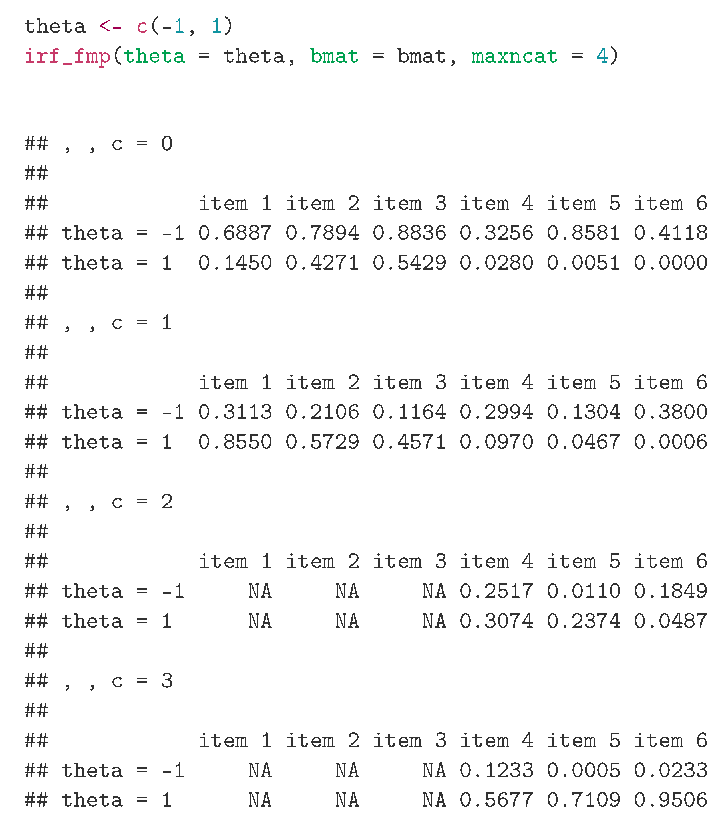Calls to irf_fmp will result in a three-dimensional array with $\theta$ values in the first dimension, items in the second dimension, and response categories in the third dimension. For example,

In the above output (and elsewhere in this tutorial), informative dimension labels have been added to ease readability. This output shows, for example, that the probabilities of responding in categories 0, 1, 2, and 3 to item 6 for a person with $\theta =-1$ equal 0.4118, 0.3800, 0.1849, and 0.0233. Notice that the output also includes some NA values. This is because items 1, 2, and 3 have only 2 response categories, and therefore these subjects can only respond in categories 0 and 1 and categories 2 and 3 are NA.

For dichotomous items, it is common to only find the probability of responding in the higher response category (because the sum of response category probabilities must sum to 1 for each $\theta$, probabilities for category 0 are 1 minus those for category 1). In flexmet, specific category response probabilities can be found by adding the returncat argument. This is illustrated below for item 1:

Notice that the maxncat argument is set equal to 4 in this example, even though the item is dichotomous. This is because the item parameters are taken from the first row of bmat, and bmat includes columns corresponding to four-category items. In other words, maxncat should be set to one greater than than the number of bmat columns (or one greater than the number of bmat entries, if bmat is a vector) that correspond to $\xi$ parameters, even if no item with maxncat categories is included in the call to bmat. Note that the returncat argument represents the value of the category to output, where categories are labeled starting at 0. Therefore, returning category “1” for dichotomous item 1 returns the probability of a positive item response to item 1. By default, if maxncat = 2, only probabilities for category “1” are returned, and if maxncat > 2, all response category probabilities are returned.

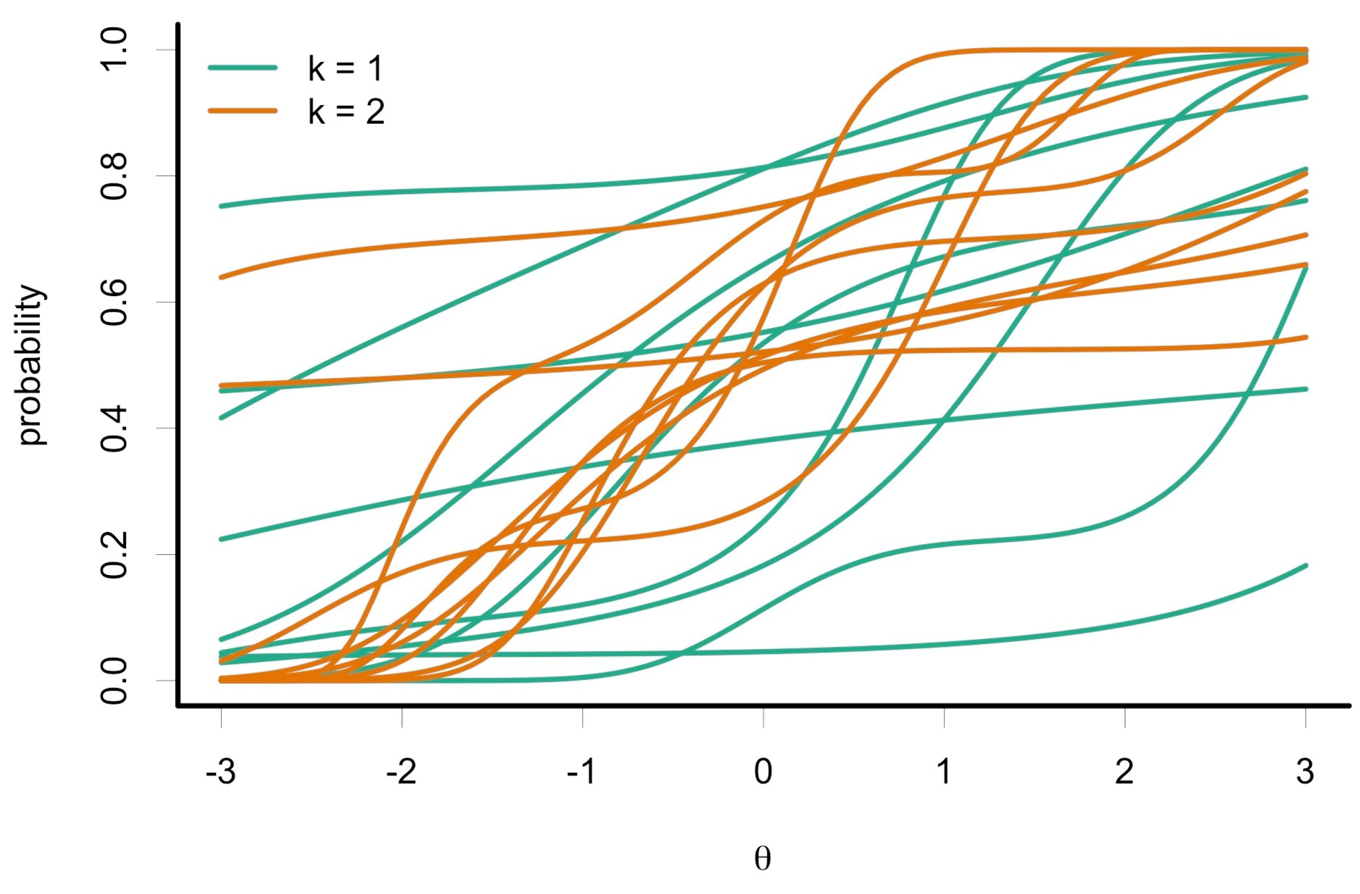
Calls to irf_fmp also can be used to plot IRFs. Figure 1 displays the IRFs for the six example items, and tge code to produce a version of this figure is included in Appendix C. In this figure, response probabilities for category 1 (a positive response) are shown for the 3 dichotomous items, and all response category probabilities are shown for the 3 polytomous items.

3. Fitting the FMP Model in flexmet

The flexmet package includes functionality for specifying, fitting, and manipulating the general FMP model. Notably, flexmet is not the only R package available for fitting the FMP model. For example, the mirt package [15] includes functionality to estimate FMP item parameters using marginal maximum likelihood estimation. However, if any items have $k=0$, the mirt package currently (version 1.34 of mirt is current at the time of writing) requires the user to estimate either 2PL or GPCM parameters rather than FMP parameters. Because mirt parameterizes the 2PL and GPCM differently than the Greek-letter FMP parameterization, this may make the mirt package less than ideal for tests with a variety of $k_i$ values and for advanced applications of the FMP model (such as scale transformations, as described in a later section). Therefore, the flexmet package includes several ways to estimate FMP model parameters, including built-in methods for fixed-effects and random-effects estimation, as well as a wrapper that uses the mirt package to estimate parameters and return parameter estimates in a standardized format. As illustrated below, flexmet facilitates item parameter estimation for items with any combination of $k_i$ values and numbers of response categories, with or without the use of Bayesian priors.

Early applications of the FMP model treated the latent trait as a fixed effect to estimate item parameters [3,11]. In this fixed-effects approach, initial estimates of the $\theta$ parameters are treated as known quantities when calculating maximum likelihood estimates of the Greek-letter parameters for an individual item. These fixed $\theta$ values are called $\theta$ surrogates  [3,11] and are calculated as the first principal components scores of the full data matrix. In the following code chunk, 1000 true $\theta$ values are simulated from a standard normal distribution. Then, the sim_data function in flexmet is used in conjunction with the six-item bmat matrix defined earlier to randomly generate item response data. Finally, $\theta$ surrogates are calculated by passing the simulated data to flexmet’s get_surrogates function.

The tsur object now includes 1000 $\theta$ surrogate values calculated from the simulated data. To estimate item parameters for a single item using fixed-effects estimation with $\theta$ surrogates, we can use the fmp_1 function in flexmet. As illustrated below, this function requires the user to specify the data vector, the desired k value, and a vector of $\theta$ surrogates tsur. Below, this is illustrated for k values of 0, 1, and 2.

The best choice of k for a given item is typically unknown, and so authors have suggested comparing the item-level Akaike Information Criteria (AIC) value to select the optimal k value [3,12]. We can perform this comparison by extracting the AIC list element from each call to fmp_1.

In this example, k = 1 leads to the lowest AIC value. Incidentally, $k=1$ is also the data-generating k value for this item (item 2), though this will not always be the case. Note that it is not always desirable to seek the “correct” $k_i$ value, but instead it may be preferable to approximate the population curve as closely as possible without overfitting the data. One measure of the similarity of item response functions is the root integrated mean squared error (RIMSE; [6,12]), which is defined here as

$$\mathrm{RIMSE}=\sqrt{\int {\left(\sum _{c=0}^{C_i-1}x{P}_1(X_i=c|\theta )-\sum _{c=0}^{C_i-1}x{P}_2(X_i=c|\theta )\right)}^{2}g\left(\theta \right)d\theta }$$

(6)

where $P_1$ and $P_2$ represent the two item response functions to compare (not necessarily from the FMP model), and $g\left(\theta \right)$ indicates a $\theta$ distribution to integrate over. Smaller values of RIMSE indicate greater similarity between the two curves. In flexmet, the rimse function can calculate the RIMSE for any combination of $\mathit{b}$-vectors that represent the same number of response categories (though not illustrated here, rimse can also be used with non-FMP item response functions). In flexmet, $g\left(\theta \right)$ is standard normal by default but can be modified using the int argument, which expects a matrix with two columns. The first column should include a sequence of quadrature points, and the second column should include the densities of each quadrature point, scaled so that the densities sum to 1. The int_mat function in flexmet facilitates the creation of this matrix. The int_mat function takes a distribution function distr (such as dnorm or dunif), a named list args of the parameters of that distribution, the lower and upper bounds of the quadrature points, lb and ub, and the number of quadrature points, npts. An example of modifying these arguments of the int_mat function is included later in this paper (Section 4.2).

The first two arguments to rimse should be two vectors of $\mathit{b}$-parameters, in either order. In the code below, the true $\mathit{b}$-parameters for item 2 are listed first. Note that because columns 2 and 3 of bmat represent category intercept parameters for polytomous items (and include NA values for item 2), we omit these from the $\mathit{b}$-vector when calling rimse. The estimated $\mathit{b}$-parameters are listed second and are found in the bmat list element of each call to fmp_1. If items are polytomous, the ncat argument should also be specified to indicate the number of response categories. Because the default value of ncat = 2, it is not necessary to include this argument for dichotomous items.

Comparing the RIMSE of the estimated curves versus the data-generating curves for 3 values of k, we see that k = 0 leads to the highest error in estimation, followed by k = 2, and k = 1 most closely traces the population item response function.

It is also possible to estimate fixed-effects item parameters for multiple items in one command using the fmp function with the em = FALSE argument. This method will automatically calculate $\theta$ surrogates based on the provided data matrix. In the fmp function, it is possible to specify different k values for different items. Namely, if a scalar is specified for the k argument, the same k value will be used for all items. Otherwise, a vector of k values should be specified, one per item.

In the example below, the fixed-effects FMP model is fit several times. First, all items are fit with $k=0$, $k=1$, and $k=2$. Based on these results, a model with differing k values is specified based on the optimal k value, as indicated by comparing item-level AIC values.

The user may notice that the model with k = 2 produces an error that the (item parameter) information matrix cannot be inverted. This is a common problem with high k values. If this error occurs, standard errors are not available for the estimated item parameters; however, the item parameter estimates themselves may be used without concern.

Based on the above results, we see that the lowest AIC value is observed for $k=$ 0, 0, 2, 2, 0, and 1 for the 6 items. We may then choose to fit a new fixed-effects FMP model with these varying k values, as illustrated below.

In the item parameter matrix printed above, notice how items with different k values and numbers of response categories are represented. Specifically, NA’s are used as placeholders for items 1–3 that include less than the maximum number of response categories. In contrast, if $k_i$ is less than the maximum $k_i$ value represented in the parameter matrix (as is the case for items 1, 2, 5, and 6), then the higher-order $\mathit{b}$ parameters are set to 0.

In addition to fixed-effects estimation, flexmet also provides functionality for random-effects estimation using marginal maximum likelihood estimation via the expectation-maximization (EM) algorithm [20]. The flexmet package includes both an inbuilt algorithm for estimating item parameters (using the fmp function with option em = TRUE) and a wrapper to the mirt [15] package (using the fmp function with option em = "mirt"). The mirt algorithm is currently faster and more reliable than the inbuilt algorithm, and so this option is used for illustration. Note that the mirt package must be installed in order to use this option. Using the same pattern of k values found with the fixed-effects model, we find the following results:

At a glance, comparing the bmat outputs of fe_mixed and re_mixed indicates that while some parameter estimates are similar across the two estimation methods, others are quite different. Notably, for highly parameterized models such as the FMP model, very different sets of parameters can trace similar curves. For this reason, it is useful to plot curves or to apply overall summary measures such as the RIMSE when comparing estimated curves to the true curve or to each other. These RIMSE values are calculated for fe_mixed and re_mixed after illustrating one final estimation method.

Another useful estimation option available for both the fmp_1 and fmp functions is the use of Bayesian priors. Particularly, for higher values of k, the FMP model may become computationally unstable, which can be somewhat alleviated through the use of priors [12]. Because the Greek-letter parameterization of the FMP is used for parameter estimation, priors are placed on the Greek-letter parameters rather than on the more readily interpretable $\mathit{b}$ parameters. When choosing priors, it may be helpful to note that $({\xi }_{1i},\dots {\xi }_{(C_i-1)i})=(b_{0_{1}i},\dots b_{0_{C_i-1}i})$ and that $\omega =ln{b}_1$. In addition, higher-order $\mathit{b}$ parameters will equal zero if the corresponding $\alpha =0$ and $\tau =-\infty$. Prior predictive simulation may help the user to select appropriate priors. For example, the following code produces a prior predictive simulation of 20 item response curves generated from the following distributions: $\xi \sim N(0,1)$, $\omega \sim N($−$0.5,1)$, $\alpha \sim N(0,0.5)$, and $\tau \sim N(-3,0.5)$. The plot produced by this code is shown in Figure 2. This choice of priors appears to allow for a variety of shapes and locations of the FMP curves, and so we continue to illustrate Bayesian estimation with these priors.

Priors can be added to models fit using flexmet by specifying the prior argument to the fmp or fmp_1 function. As of version 1.1 of flexmet, only normally distributed priors are available, and the same priors are applied to all model parameters of a given class (i.e., for all items in the data set and for all instances of that parameter type within an item). To specify priors, a list with named elements xi, omega, alpha, and tau should be passed to the prior argument. For example, to specify a standard normal prior for all $\xi$s, we may write prior = list(xi = c("norm", 0, 1)). The code below illustrates Bayesian estimation with the em = "mirt" option.

Finally, we may compare the accuracy of each of the three illustrated estimation methods using the rimse function. The code below does this for each of the six simulated items. For each item, random-effects estimation tends to lead to somewhat more accurate curves than fixed-effects estimation, and the use of priors improves parameter estimation accuracy in some, but not all, cases.

Several other estimation options are available with the fmp and fmp_1 functions that are not illustrated here. A vector of starting values may be specified with the start_vals argument, where parameters should be listed in the same order as the estimated parameters given in the parmat list element of the fitted model object. For fixed-effects estimation, the method argument indicates the optimization algorithm (passed to the optim function in R’s stats package). For random-effects estimation, the max_em option indicates the maximum number of EM cycles (default 500), and the n_quad function indicates the number of quadrature points (default 49). Additional named arguments may be passed to the optim function (if em = TRUE) or the mirt function (if em = "mirt").

Finally, flexmet includes the th_est_ml and th_est_eap functions for maximum likelihood (ML) and expected a posteriori (EAP, [21]) person parameter estimation. Both of these functions require a data matrix dat and a matrix of $\mathit{b}$-parameters bmat. If at least one item is polytomous, the maxncat argument should also be specified. By default, the th_est_eap function uses a standard normal prior with 33 quadrature points, and this may be modified using the int argument in conjunction with int_mat. A call to either trait estimation function will result in a matrix with two columns: one for the $\theta$ parameter estimates and one for the standard errors (for ML) or posterior standard deviations (for EAP). The code below illustrates this procedure for the example data and the re_priors estimated item parameters.

4. Transforming the FMP Model with flexmet

Aside from the increased flexibility in IRF shapes afforded by the FMP model, another potential use of the FMP model is to transform item response models linearly or nonlinearly [18,19]. Specifically, suppose that two scalings of the latent trait, $\theta$ and ${\theta }^{★}$, are related by a monotonic polynomial function of degree $2k_{\theta }+1$ such that

$$\theta =t_0+t_1{\theta }^{★}+t_2{\theta }^{★2}+\cdots t_{2k_{\theta }+1}{\theta }^{★2k_{\theta }+1},$$

(7)

where $k_{\theta }$ is a non-negative integer. Then, an FMP model defined on the scale of $\theta$ may be transformed to the scale of ${\theta }^{★}$ using matrix operations described elsewhere [18,19]. For a given $k_{\theta }$ and an item with a given $k_i$ (i.e., item complexity defined on the scale of $\theta$), the item complexity on the scale of ${\theta }^{★}$, $k_i^{★}$, equals

$$k_i^{★}=2k_i{k}_{\theta }+k_i+k_{\theta }.$$

(8)

Therefore, item response functions on the scale of ${\theta }^{★}$ will necessarily have larger item complexities than response functions on the scale of $\theta$.

Two applications of nonlinearly transforming the FMP model will be illustrated below. In the first application, item parameters are estimated separately for two groups with different latent trait distributions. Because the latent trait is often assumed to follow a standard normal distribution for model identification, the fitted item response models will be on different, nonlinearly related, scales. Linear and nonlinear linking transformations will be estimated and compared. In the second application, an item response model will be transformed such that the latent trait scale is on a more interpretable percentage-correct score metric.

4.1. Item Parameter Linking with the FMP Model

If item parameters for the same items are estimated from two different samples, item parameter linking may be used to put the parameters on the same scale. The need for item parameter linking arises from differences in model identification constraints [22]. For the most common parametric item response models, such as the 2PL and GPCM, the chosen functional form of the item response model identifies the scale of the latent trait up to a linear transformation. In addition, models may be identified by assuming that the latent trait is standardized, or that the latent trait follows a standard normal distribution (as is the case for the fixed-effects FMP estimation illustrated above). Therefore, if there are any differences in the location, variance, or shape of the latent trait distribution between groups, linking may be necessary to put the two sets of item parameters on more similar scales. To illustrate how item parameters on different scales may be linked with the FMP model, an illustrative simulation is presented next.

To simulate data, a population set of FMP item parameters was first generated for 20 items each with two response categories and $k=0$ using the sim_bmat function in flexmet. With the sim_bmat function, the user can generate items with varying k values and numbers of response categories by specifying vectors for the k and ncat functions. The population item parameters were then used to generate data for two groups of 5000 examinees. The population latent trait values for the first group were first drawn from a standard normal distribution, then transformed by taking −2 plus e to the power of the standard normal scores divided by 2. The population latent trait values for the second group were drawn from a standard normal distribution. From this design, because the second group’s $\theta$ values were transformed to the scale of the first group’s scores (which were identified by a combination of the shape of the fitted model and the assumption of a standard normal distribution), the population relationship between the two scales equals

$$\theta =-2+exp({\theta }^{★}/2).$$

(9)

After generating population $\theta$ values, data were then generated separately for each group. To select the k values that best represent these data, each item for each group was first fit to a series of FMP models using the fmp_1 function based on theta surrogates. Specifically, each item was first fit with $k=0$ and $k=1$. If the AIC for $k=0$ was smaller than for $k=1$, then the final model was fit with $k=0$. If not, models with sequentially higher k values were fit until the model with the smaller k value had a smaller AIC than the model with the higher k value. The code to implement this procedure is included in Appendix D and resulted in a mixture of $k=0$ and $k=1$ for both groups. Once the empirically selected k values for each item and group were chosen, item parameters were estimated again with fmp and the em = "mirt" option. For group 1, the argument technical = list(NCYCLES = 1500) was passed to mirt because more than 500 cycles of the EM algorithm (the default in mirt) were required for this model to converge.

The flexmet package includes two functions for linking item parameters: hb_link for linking based on the Haebara method (HB) [23] and sl_link for linking based on the Stocking–Lord method (SL) [24], and both functions take the same arguments. The bmat1 and bmat2 arguments give the matrices of item parameters in the polynomial coefficient parameterization. These functions currently assume that both matrices include the same set of common items in the same order. The bmat2 parameters are on the ${\theta }^{★}$ metric and are transformed to the $\theta$ metric of the bmat1 parameters. The polynomial degree of the estimated transformation is specified by the k_theta argument (monotonicity of the estimated linking transformation is ensured using the same strategy as is used for item parameters).

From the objects returned by calls to hb_link and sl_link, the value list element gives the function value from minimizing the HB or SL criterion (see [23,24] for details). Comparing these values resulting from the HB or SL method with different $k_{\theta }$ can help inform which $k_{\theta }$ yields the most appropriate latent trait transformations, where smaller values indicate smaller differences between the estimated item/test response functions on the two scales. Although criteria values from calls to hb_link should not be compared to values from calls to sl_link, comparing values with different $k_{\theta }$ suggests that $k_{\theta }=1$ leads to the closest match between the two sets of item parameters under both the SL and HB methods.

Calls to hb_link and sl_link also output the estimated vector of polynomial coefficients in the tvec list element. As shown below, although these values are similar for the HB and SL methods, there are some differences, particularly for higher-order polynomial coefficients.

The tvec output is useful for understanding the estimated relationship between the $\theta$ and ${\theta }^{★}$ scales. Recall from Equation (7) that $\theta$ is a polynomial function of ${\theta }^{★}$, and Equation (9) gives the population relationship between $\theta$ and ${\theta }^{★}$. In Figure 3, the SL linking transformations are compared to the true linking transformation. The code to reproduce a version of this figure is included in Appendix E and makes use of flexmet’s inv_poly function to calculate the $\theta$ value that corresponds to any particular value of ${\theta }^{★}$. Although in non-simulation applications, the true latent trait transformation will not be known, plotting may still be a useful tool to inspect the similarity of different transformations.

To illustrate the meaning of the linking transformation, consider a $\theta$ value of 0.5. In the code below, this $\theta$ value is transformed to a ${\theta }^{★}$ value using the inv_poly function, which takes a scalar value (here, each $\theta$) and returns the ${\theta }^{★}$ value that combines with the polynomial coefficient vector coefs (see Equation (7)) to produce $\theta$. As shown below for the SL transformation with $k_{\theta }=1$, the item response probabilities for theta combined with the originally estimated bmat are identical to the transformed thetastar values combined with the transformed item parameters (which are found in the bmat list element of the linking output). This equality is demonstrated for the first three items of the simulated test.

4.2. Transforming the FMP Model to a User-Defined Scale

Another potential application of FMP model transformations is to specify an item response model on a latent trait metric other than $\theta$. In the following illustration, flexmet functions are used to transform a set of 3 parameter logistic (3PL) model item parameters from the typical $\theta$ metric to a percentage-correct (PC) metric where the lowest score is 0, the highest score is 100, and scores roughly correspond to the percentage of items answered correctly. Although this type of model transformation is illustrated using a PC metric, any monotonic transformation is possible, so long as the user can identify a suitable polynomial approximation to the desired transformation. Transforming the entire item response model to a more interpretable metric allows for trait estimates, item information, standard errors, and other quantities to be calculated directly on the reported score metric.

The item parameters used for the following illustration are taken from the tcals data set found in version 3.16 of the catR package [25] (and also included in Appendix F). Note that these parameters correspond to the following representation of the 3PL model:

$$P(X_{ij}=1|{\theta }_j,a_i^{★},b_i^{★},c_i^{★})=c_i^{★}+\frac{1-c_i^{★}}{1+exp(-a_i^{★}({\theta }_j-b_i^{★}))},$$

(10)

where $a_i^{★}$ indicates the item discrimination parameter, $b_i^{★}$ indicates the item difficulty parameter, and $c_i^{★}$ indicates the guessing, or lower asymptote, parameter. The star notation is used for these item parameters only to avoid confusion with previously defined notation.

Note that the 3PL presented in Equation (10) is not a special case of the FMP model as presented in Equation (1). However, for dichotomous item responses, an FMP model may be specified that includes upper ($d_i^{★}$) and/or lower ($c_i^{★}$) asymptotes on the item response functions [26] as follows:

$$P(X_{ij}=1|{\theta }_j{\mathit{b}}_i,c_i^{★},d_i^{★})=c_i^{★}+\frac{d_i^{★}-c_i^{★}}{1+exp(-b_0-m^{★}({\theta }_j,b_{1i},\dots ,b_{2k_i+1,i}))}.$$

(11)

If not otherwise specified, we may assume that all $d_i^{★}=1$ and all $c_i^{★}=0$. In many flexmet functions, upper and lower asymptote parameters may be specified using the cvec and dvec arguments (note that flexmet currently does not allow these asymptote parameters to be estimated with the fmp or fmp_1 functions; however, most other flexmet functions accommodate asymptote parameters). These asymptote parameters are unaffected by transformations of the latent trait metric.

In the code below, the tcals parameters are read in first. Then, an object fmp_pars is defined that transforms the 3PL $a_i^{★}$ and $b_i^{★}$ parameters to the polynomial coefficients required by the FMP model. Then, a sequence of $\theta$ values is generated between −4 and 4, and item response probabilities are calculated for each item and $\theta$ value. The expected percentage-correct (PC) scores are then calculated by summing the item response probabilities for each $\theta$ value and multiplying them by $100/85$ (where 85 is the number of test items). We then regress the $\theta$ values on the PC scores using monotonic polynomial regression [27] as implemented in version 0.3–10 of the Monopoly package [28] for R. Several regressions are fit using k values (which are used as $k_{\theta }$ values) from 0 to 5, where, as before, $2k+1$ indicates the maximum polynomial degree. Finally, the average regression residual is printed for each k value.

The average regression residuals indicate that higher k values lead to better approximations of the desired curve. However, choosing a higher k value will lead to many higher-order coefficients for the transformed item parameters, so we may choose to use the smallest k value that yields an acceptable level of accuracy. For instance, if we decide that an average regression residual of less than 0.1 is acceptable, then we may choose to move forward with the $k=1$ transformation. The estimated regression coefficients then become the polynomial coefficients with which to transform fmp_pars (i.e., the t coefficients for Equation (7) with $k_{\theta }=1$). We can implement this transformation by applying the transform_b function in flexmet to each row of fmp_pars, specifying the $\theta$ transformation coefficients in the tvec argument, as illustrated below.

Note again that the $c_i^{★}$ parameters remain unchanged during FMP parameter transformations, and so the argument cvec = tcals$c should be passed to any flexmet function that makes use of these parameters. For example, we may compare two methods of calculating trait estimates on the transformed ${\theta }^{★}$/PC metric: first, estimating person parameters on the $\theta$ metric and then applying the polynomial transformation; and estimating person parameters directly on the ${\theta }^{★}$/PC metric. In this example, we use a standard normal prior to estimate EAPs on the $\theta$ metric, and a $N(80,10)$ prior to estimate EAPs directly on the ${\theta }^{★}$/PC metric. This prior is specified by feeding the output of a call to the int_mat function to the int argument. In the example code shown below, both priors are specified with 89 quadrature points, the prior on $\theta$ is bounded between 0 and 4, and the prior on ${\theta }^{★}$ is bounded between 0 and 100. Finally, the EAPs that were estimated on the $\theta$ metric are transformed to the ${\theta }^{★}$/PC metric using the inv_poly function.

Comparing the distribution of trait estimates calculated with both approaches, we see that the scores are relatively similar (the small difference in estimated distributions may be due to the use of different prior distributions). However, a major advantage of estimating parameters directly on the ${\theta }^{★}$/PC metric is that the estimated standard errors are on the appropriate metric. That is, nonlinear monotonic transformations of the latent trait metric can lead to unexpected distortions of the information matrices [19,29]. An illustration of the effects of this transformation is illustrated in Figure 4, and the code to reproduce a version of this figure is included in Appendix F. This code makes use of the iif_fmp function in flexmet, which has similar arguments to the irf_fmp function and yields item information for any FMP items and $\theta$ values. In the upper panels of Figure 4, three example IRFs (taken from the 85 tcals items) are displayed on the $\theta$ metric and after being transformed to the ${\theta }^{★}$/PC metric. Notice that although the shape of each IRF changes, the relative relationships among the three curves do not change. In the bottom panels, the test information function (i.e., the sum of item-level information functions) is illustrated for both the $\theta$ and ${\theta }^{★}$ metrics. Whereas test information on the $\theta$ metric is unimodal and centered just below $\theta =0$, the ${\theta }^{★}$ metric is bimodal with peaks around ${\theta }^{★}=35$ and ${\theta }^{★}=90$. This result implies that the items that the trait regions measured most accurately on the $\theta$ metric are not necessarily those measured most accurately on the ${\theta }^{★}$ metric. This result also highlights the importance of calculating information directly on the metric on which scores are reported.

5. Summary

This paper provides an introduction to the specification and use of the FMP model through the flexmet package for R. Version 1.1 of flexmet includes functionality to estimate FMP item parameters for both dichotomous and polytomous items, as well as methods to transform FMP item parameters, generate FMP item parameters and data, and several other methods that are particularly useful when working with the FMP model. The provided examples also illustrate some scenarios in which it may be desirable to use the FMP model, including fitting IRFs that can take on more flexible shapes than allowed by traditional models and transforming item response models to user-defined metrics (e.g., a sum score or proportion-correct metric). Moreover, it is hoped that broader use of the flexmet package will lead to further development of the flexmet package, including planned features such as more choices of prior distributions for Bayesian estimation and the estimation of upper and lower asymptote parameters. Although not every feature of the current flexmet package is illustrated in the examples presented above, we hope that this tutorial provides the reader with an accessible introduction to the FMP model and the tools to use the FMP model with the flexmet package.

References

1. Birnbaum, A. Some latent trait models and their use in inferring an examinee’s ability. In Statistical Theories of Mental Test Scores; Lord, F., Novick, M., Eds.; Addison-Wesley: Reading, MA, USA, 1968; pp. 397–479. [Google Scholar]
2. Molenaar, I.W. Thirty years of nonparametric item response theory. Appl. Psychol. Meas. 2001, 25, 295–299. [Google Scholar] [CrossRef] [Green Version]
3. Liang, L.; Browne, M.W. A quasi-parametric method for fitting flexible item response functions. J. Educ. Behav. Stat. 2015, 40, 5–34. [Google Scholar] [CrossRef]
4. Ramsay, J.; Winsberg, S. Maximum marginal likelihood estimation for semiparametric item analysis. Psychometrika 1991, 56, 365–379. [Google Scholar] [CrossRef]
5. Mokken, R.J. A Theory and Procedure of Scale Analysis; De Gruyter Mouton: Berlin, Germany; New York, NY, USA, 2011. [Google Scholar]
6. Ramsay, J.O. Kernel smoothing approaches to nonparametric item characteristic curve estimation. Psychometrika 1991, 56, 611–630. [Google Scholar] [CrossRef]
7. Falk, C.F.; Feuerstahler, L.M. On the Performance of Semi-and Nonparametric Item Response Functions in Computer Adaptive Tests. Educ. Psychol. Meas. 2021. [Google Scholar] [CrossRef]
8. Xu, X.; Douglas, J. Computerized adaptive testing under nonparametric IRT models. Psychometrika 2006, 71, 121–137. [Google Scholar] [CrossRef]
9. Falk, C.F.; Fischer, F. More flexible response functions for the PROMIS physical functioning item bank by application of a monotonic polynomial approach. Qual. Life Res. 2021, 1–11. [Google Scholar] [CrossRef]
10. Wiberg, M.; Ramsay, J.O.; Li, J. Optimal scores: An alternative to parametric item response theory and sum scores. Psychometrika 2019, 84, 310–322. [Google Scholar] [CrossRef] [PubMed]
11. Liang, L. A Semi-Parametric Approach to Estimating Item Response Functions. Ph.D. Thesis, The Ohio State University, Columbus, OH, USA, 2007. [Google Scholar]
12. Falk, C.F.; Cai, L. Maximum marginal likelihood estimation of a monotonic polynomial generalized partial credit model with applications to multiple group analysis. Psychometrika 2016, 81, 434–460. [Google Scholar] [CrossRef] [PubMed] [Green Version]
13. Muraki, E. A Generalized Partial Credit Model: Application of an EM Algorithm. Appl. Psychol. Meas. 1992, 16, 159–176. [Google Scholar] [CrossRef]
14. Rizopoulos, D. ltm: An R package for Latent Variable Modelling and Item Response Theory Analyses. J. Stat. Softw. 2006, 17, 1–25. [Google Scholar] [CrossRef] [Green Version]
15. Chalmers, R.P. mirt: A multidimensional item response theory package for the R environment. J. Stat. Softw. 2012, 48, 1–29. [Google Scholar] [CrossRef] [Green Version]
16. Robitzsch, A.; Kiefer, T.; Wu, M. TAM: Test Analysis Modules; R Package Version 3.7-16. 2021. Available online: https://search.r-project.org/CRAN/refmans/TAM/html/TAM-package.html (accessed on 16 August 2021).
17. Elphinstone, C. A target distribution model for nonparametric density estimation. Commun. Stat.-Theory Methods 1983, 12, 161–198. [Google Scholar] [CrossRef]
18. Feuerstahler, L. Exploring Alternate Latent Trait Metrics with the Filtered Monotonic Polynomial IRT Model. Ph.D. Thesis, University of Minnesosta, Minneapolis, MN, USA, 2016. [Google Scholar]
19. Feuerstahler, L.M. Metric transformations and the filtered monotonic polynomial item response model. Psychometrika 2019, 84, 105–123. [Google Scholar] [CrossRef]
20. Bock, R.D.; Aitkin, M. Marginal maximum likelihood estimation of item parameters: Application of an EM algorithm. Psychometrika 1981, 46, 443–459. [Google Scholar] [CrossRef]
21. Bock, R.D.; Mislevy, R.J. Adaptive EAP estimation of ability in a microcomputer environment. Appl. Psychol. Meas. 1982, 6, 431–444. [Google Scholar] [CrossRef]
22. Van der Linden, W.J.; Barrett, M.D. Linking item response model parameters. Psychometrika 2016, 81, 650–673. [Google Scholar] [CrossRef] [Green Version]
23. Haebara, T. Equating logistic ability scales by a weighted least squares method. Jpn. Psychol. Res. 1980, 22, 144–149. [Google Scholar] [CrossRef] [Green Version]
24. Stocking, M.L.; Lord, F.M. Developing a common metric in item response theory. Appl. Psychol. Meas. 1983, 7, 201–210. [Google Scholar] [CrossRef] [Green Version]
25. Magis, D.; Barrada, J.R. Computerized adaptive testing with R: Recent updates of the package catR. J. Stat. Softw. 2017, 76, 1–19. [Google Scholar] [CrossRef]
26. Falk, C.F.; Cai, L. Semiparametric item response functions in the context of guessing. J. Educ. Meas. 2016, 53, 229–247. [Google Scholar] [CrossRef]
27. Murray, K.; Müller, S.; Turlach, B.A. Revisiting fitting monotone polynomials to data. Comput. Stat. 2013, 28, 1989–2005. [Google Scholar] [CrossRef]
28. Murray, K.; Müller, S.; Turlach, B. Fast and flexible methods for monotone polynomial fitting. J. Stat. Comput. Simul. 2016, 86, 2946–2966. [Google Scholar] [CrossRef]
29. Lord, F.M. Applications of Item Response Theory to Practical Testing Problems; Erlbaum: New York, NY, USA, 1980. [Google Scholar]
Figure 1. Item response functions for six example FMP items. Items 1, 2, and 3 are dichotomous, and items 4, 5, and 6 have four response categories. Items 1 and 4 have k i = 0 , items 2 and 5 have k i = 1 , and items 3 and 6 have k i = 2 .
Psych 03 00031 g001
Figure 2. Prior predictive simulation of FMP item response curves with k = 1 and k = 2 and ξ N ( 0 , 1 ) , ω N ( 0.5 , 1 ) , α N ( 0 , 0.5 ) , and τ N ( 3 , 0.5 ) .
Psych 03 00031 g002
Figure 3. True linking transformation and estimated Stocking–Lord linking transformations with various k θ values.
Psych 03 00031 g003
Figure 4. Item response functions (upper row) and test information functions (bottom row) on the original θ metric and on the transformed percentage-correct metric θ .
Psych 03 00031 g004