Between-Item Multidimensional IRT: How Far Can the Estimation Methods Go?

Abstract

Multidimensional item response models are known to be difficult to estimate, with a variety of estimation and modeling strategies being proposed to handle the difficulties. While some previous studies have considered the performance of these estimation methods, they typically include only one or two methods, or a small number of factors. In this paper, we report on a large simulation study of between-item multidimensional IRT estimation methods, considering five different methods, a variety of sample sizes, and up to eight factors. This study provides a comprehensive picture of the methods’ relative performance, as well as each individual method’s strengths and weaknesses. The study results lead us to make recommendations for applied research, related to which estimation methods should be used under various scenarios.

1. Introduction

Given the known difficulties with estimating multidimensional item response theory (MIRT) models [1], the goal of this paper was to compare a variety of estimation methods across a large range of sample size and model size conditions in a simulation study. Our objective is to provide recommendations to applied researchers regarding which estimation method is better suited across different types of research contexts.

For dichotomous indicators, unidimensional IRT models express the probability of endorsing an item (e.g., giving a correct response) as a function of a common underlying/unobserved factor and a set of item parameters. There are multiple IRT models for dichotomous items that differ in terms of their item parameters. The two-parameter logistic model (2PL), which is the model of focus in this paper, is one of the most common IRT models for dichotomous responses. The probability of endorsing item j for each subject i can be expressed as

$$P(u_{ij}=1|{\theta }_i)=\frac{1}{1+exp(-a_j({\theta }_i-b_j))}$$

(1)

In Equation (1), $u_{ij}$ is the item response 0 or 1, and ${\theta }_i$ represents the underlying factor score for each subject i. The 2PL model includes a discrimination/slope parameter $a_j$ for each item j, indicating that items can have different degrees of relation with $\theta$. The $b_j$ parameter represents the location/threshold for each item j, which tells us at what point on the latent variable continuum the item is most discriminating [1,2].

IRT models were initially developed under the assumption of unidimensionality, meaning that a single latent variable underlies the probability of item responses. This assumption has been questioned as inappropriate for complex phenomena, and is perhaps an unrealistic representation of item responses. In fact, some have argued that every test is multidimensional to some degree [3], necessitating multidimensional IRT (MIRT) models (e.g., [4]).

There are two types of multidimensionality commonly discussed within the MIRT literature. Between-item multidimensionality occurs when each item measures a single construct, but multiple constructs are measured by the set of items. This is in contrast to within-item multidimensionality, which occurs when a single item reflects variation on more than one underlying construct [5]. In the current project, we focused solely on between-item multidimensional models, which is relevant to applications in which there is a theoretical basis for distinct factors. Within-item multidimensional models, while also an important area of research, are not considered here.

MIRT Model

For this project, we focus on the 2PL IRT model for dichotomous items. The 2PL MIRT is an straightforward extension of the unidimensional model (Equation (1)) and can be represented with two common parameterizations: slope-intercept and slope-threshold. Here, we work with the slope-threshold formulation

$$P(u_{ij}=1|{\mathit{\theta }}_{ik})=\frac{1}{1+exp(-{\mathit{a}}_j^{\prime }({\mathit{\theta }}_i-{\mathit{b}}_j))},$$

(2)

for which P is the predicted probability of answering 1, $u_{ij}$ is the item response (1 for endorsement, and 0 otherwise) for subject i on item j, and ${\mathit{\theta }}_i$ is the vector of factor scores for subject i. Additionally, ${\mathit{a}}_j$ and ${\mathit{b}}_j$ can be conceptualized as slope/discrimination and threshold parameters for item j, which matches the form of the unidimensional model. Each slope parameter indicates the magnitude of the relation between item j and the respective factor, while the threshold indicates at what level of the respective latent variable $\theta$ each item’s slope is the steepest. In the between-item multidimensional model, each item j has one free parameter in the ${\mathit{a}}_j$ vector, while the within-item model involves multiple free parameters in ${\mathit{a}}_j$ that representing the relationships between the item j and each factor that defines item j.

For multidimensional models, the formulation from Equation 2 includes redundant parameters that help us see similarities to the unidimensional model, but that are not identified. Instead of estimating multiple ${\mathit{b}}_j$ parameters per item, we simply estimate a scalar parameter that equals ${\mathit{a}}_j^{\prime }{\mathit{b}}_j$. We further identify the model by fixing the factor means to 0 and the factor variances to 1.

Commonly, these IRT models are estimated with marginal maximum likelihood (MML) estimation based on the expectation maximization (EM) algorithm. More recently, a variation of Markov chain Monte Carlo (MCMC) sampling for Bayesian inference has been used, as well as methods that combine the advantages of MCMC sampling with ML estimation, such as Quasi-Monte Carlo EM integration (QMCEM) and Metropolis–Hastings Robbins–Monro (MHRM).

Within a factor analytic framework, the latent variable models for dichotomous items are often conceptualized as item factor analysis (IFA) models. IFA is an adaptation of the factor analysis model for continuous items. These are usually limited information methods, as they involve the estimation of bivariate item relations such as tetrachoric or polychoric correlations [6]. This is in contrast to IRT estimation methods, which use all the available information in the item responses and not just summary statistics (i.e., the item covariance matrix) [1,7].

Factor analysis parameter estimation typically includes the use of weighted least squares (WLS) in combination with tetrachoric or polychoric correlation matrices to estimate SEM models based on limited information. Estimation methods have been compared for unidimensional models [8], as well as for multidimensional models with few factors and large sample size [9]. In general, previous studies comparing estimation methods have either compared only a handful of estimation methods, or when more estimation methods are compared, they focused on few simulation conditions with large sample sizes [6,8,9,10,11,12,13,14,15]. To our knowledge, there is no clear information about the comparison between these estimation methods for highly multidimensional models and a large range of sample sizes.

The goal of the present research was to compare different estimation methods with a Monte Carlo simulation. Specifically, we were interested in how the methods perform across different numbers of factor and sample sizes for between-item multidimensional 2PL models. The results can help in providing guidelines for researchers who wish to fit MIRT models.

In the following pages, we first provide an overview of the estimation methods that we compared in the simulation study. We then describe the design of the simulation study and the estimation methods that will be evaluated. Then, we present the results of the simulation study, comparing each estimation method. Lastly, we provide a discussion of the results, focusing on recommendations for applied researchers and future directions for related research.

2. Estimation Methods

This project focuses on five estimation methods. The first four are frequentist, including three IRT full information methods (EM, QMCEM, and MHRM) and one limited information method (SEM-WLSMV). The last method is Markov chain Monte Carlo (MCMC) sampling for Bayesian inference. A description of the methods is provided below.

2.1. Expectation-Maximization (EM)

Marginal maximum likelihood (MML) was developed by [16] as a two-step approach for full information parameter estimation. The model likelihood defines the joint probability of the item response pattern given the subject parameters. MML subjects are random effects, and the respective marginal probability of observing each response pattern is derived by integrating the subject effect out of the joint likelihood. In doing so, the subject and item parameters are separated. MML estimates item parameters with the expectation-maximum (EM) algorithm, and the subject parameters can be estimated afterward from the item parameters.

The EM algorithm is an iterative procedure useful to approximate MML estimates in incomplete data problems. Define $\mathit{y}$ as a vector of observed data, with $\mathit{u}$ as a vector of unobserved data, and $\mathit{\xi }$ as a vector of parameters. Then we have that $f(\mathit{y},\mathit{u};\mathit{\xi })$ is the joint density of the complete data $(\mathit{y},\mathit{u})$. The likelihood of interest is marginalized out from the unobserved data as $L(\mathit{\xi };\mathit{y})=\int f(\mathit{y},\mathit{u};\mathit{\xi })\partial \mathit{u}$. At each iteration, the EM algorithm performs an expectation and maximization step. At each tth iteration of the algorithm, the E-step computes the conditional expectation of the complete data log-likelihood, conditional on the observed data and the current parameter value. Then the M-step takes the updated parameters ${\mathit{\xi }}^t$ and maximizes the complete data log-likelihood for all $\mathit{\xi }$ in the parameter space. The M-step is commonly implemented with numerical methods like Newton–Raphson [17].

2.2. Quasi-Monte Carlo EM (QMCEM)

With the EM algorithm, the E-step can involve the estimation of a high dimensional integral, which is analytically intractable. As a solution the Monte Carlo EM (MCEM) algorithm was proposed, which estimates the intractable integral with an empirical average based on simulated data [18]. Most commonly, the simulated data are generated from random draws of the distribution commanded by EM. Following the law of large numbers, this estimated integral can be highly accurate by increasing the number of simulations. This method usually requires a large number of iterations [17].

The efficiency of MCEM could be improved with simulation strategies that produce high accuracy while requiring fewer simulations. Random simulations result in inefficient data, as these random simulations fail to explore the sample space properly [19]. These limitations have led to the development of deterministic methods known as Quasi-Monte Carlo (QMC).

Monte Carlo sampling selects random uniformly distributed values across the sample space and later approximates the integral based on the empirical average. Quasi-Monte Carlo methods select the starting point deterministically. QMC produce a deterministic sequence of integral values that provide the best possible spread in the sample space. These sequences are referred to as low-discrepancy sequences [17].

In QMC, the analytically intractable expectation from EM is replaced by the empirical average, as the QMCEM updated estimates maximize the data log-likelihood conditional on the observed data and the current parameter values. Laplace importance sampling is used to find an importance sampling distribution with mean ($\mathit{\mu }\left(\mathit{\xi }\right)$) and variance ($\mathbf{\Sigma }\left(\mathit{\xi }\right)$) that match the curvature of the density distribution for the unobserved data, conditional on observed data and estimated parameters. This Laplace sampling distribution is then randomly sampled based on the chosen low-discrepancy sequence. Each of these draws is shifted and scaled by $\mathit{\mu }\left(\mathit{\xi }\right)$ and $\mathbf{\Sigma }\left(\mathit{\xi }\right)$, resulting in independent randomized sequences [17]. QMCEM overcomes the EM estimation problems that are associated with increasing dimensionality by substituting the quadrature points for the sampling distribution generated by the QMC process.

2.3. Metropolis–Hastings Robbins–Monro (MHRM)

MHRM [20,21] was developed by combining the Metropolis–Hastings MCMC (MH) sampler with the Robbins–Monro [22] technique to facilitate maximum likelihood. It is a data-augmented Robbins–Monro (RM) type [22] stochastic approximation (SA) algorithm guided by the random draws by the Metropolis–Hastings sampler.

The RM algorithm is a root-finding algorithm for noise-corrupted regression functions. MHRM extends it to multiparameter problems with stochastic augmentation of missing data. Each iteration follows three stages: (a) stochastic imputation, in which m sets of complete data are generated with the MH sampler; (b) stochastic approximation, in which the approximation of the conditional expectation for the complete data information matrix is computed; and (c) Robbins–Monro update, where the new parameters are updated with the RM algorithm. MHRM avoids the curse of dimensionality, as the stochastic imputation replaces the deterministic Gaussian quadrature from the EM algorithm [16,20].

Previous research has shown that MML has issues in estimating multidimensional IRT models, as they became computationally intensive and often intractable with a large number of factors [20,21,23]. MHRM was designed as a better alternative to MML and can provide parameter estimates for high dimensional models, models with a large number of items, or models with missing data.

2.4. Structural Equation Modeling (SEM) Approach

Structural equation modeling (SEM) approaches traditionally use limited information estimation methods. While there are several options, here we describe the most commonly used method when the items are categorical. When the indicators are continuous, the product-moment-based variance–covariance matrix serves as the input data, as the model intends to replicate the indicator relations represented by this matrix. This is helped by the assumption that ordinal observed variables follow an unobserved continuous distribution that leads to the ordinal observations, the latent response distribution (LRD, $y^{\ast }$) [24]. The relation between an observed categorical variable, y, and its respective latent response variable is represented by

$$y=c,\mathrm{if}{\tau }_c<y^{\ast }<{\tau }_{c+1}$$

(3)

As the latent value increases to the point that a discrete threshold ($\tau$) is crossed on the latent response variable ($y^{\ast }$), the observed discrete categorical value of y changes. Once this relation has been established, SEM models follow the same general structure as with continuous indicators. For example, the model-implied covariance matrix for the models considered here could be written as

$${\mathbf{\Sigma }}_{\mathit{xx}}^{\ast }\left(\mathit{\xi }\right)={\Lambda }_{\mathit{x}}^{\ast }{\Phi }_{\mathit{\zeta }\mathit{\zeta }}^{\ast }{\Lambda }_{\mathit{x}}^{\ast \prime }+{\Theta }_{\mathit{\delta }\mathit{\delta }}^{\ast },$$

(4)

which is similar to that used in confirmatory factor analysis.

Specifically, the implied variance–covariance matrix (${\mathbf{\Sigma }}_{\mathit{xx}}^{\ast }\left(\mathit{\xi }\right)$) is a function of the factor loading matrix (${\Lambda }_{\mathit{x}}^{\ast }$), latent variances and covariances (${\Phi }_{\mathit{\zeta }\mathit{\zeta }}^{\ast }$), and the diagonal matrix of unique variances (${\Theta }_{\mathit{\delta }\mathit{\delta }}^{\ast }$). When the indicators are binary, Equation (4) is equivalent to the multidimensional 2PL IRT model in Equation (2).

As the product-moment variance–covariance matrix is not appropriate for categorical indicators, a common alternative is to use the polychoric correlation matrix. This models the linear association between two continuous latent response variables based on categorical observed variables [24]. Even when we have the polychoric variance–covariance matrix, which represents the relations among the latent response variables, the traditional ML estimation is not appropriate. The alternative has been to use a distribution-free estimator from the weighted least squares (WLS) family, as it includes calculations of kurtosis in the estimation [6,24,25].

The WLS estimator still presents problems as sample size decreases and model complexity increases [6], requiring the use of robust methods for it to work efficiently. The common robust WLS methods are referred as diagonally weighted least squares (DWLS). Rather than inverting the full-weight matrix, these methods involve the inversion of only the diagonal elements of the weight matrix. Computation of the asymptotic covariance matrix of the estimated parameters uses both the diagonal and the full asymptotic variance–covariance matrix of the polychoric input matrix, but does not use the inverse of the full matrix [6,12]. Of the different robust DWLS methods, we chose to include the mean- and variance-adjusted WLS (WLSMV), which uses DWLS for parameter estimation and adjusts the fit indices and standard errors by the full weighted matrix. This method presents robust standard errors, parameter estimates, and fit indices, and it has been shown to recover population parameters in previous research [6].

As previously discussed, this model presents results according to the SEM parameterization, as in Equation (4). Note that for the other estimation techniques considered, the model is represented in the IRT parameterization. Further, the SEM is estimated with a probit link function, while the IRT models use the logit link function. To set the parameters in the same metric, as in Equation (2), we transformed the SEM parameters into the IRT metric,

$$a_j=\frac{{\lambda }_j}{\sqrt{1-{\lambda }_j^2}}\times 1.702$$

(5)

$$b_j=\frac{{\tau }_j}{{\lambda }_j}$$

(6)

where ${\lambda }_j$ represents the factor loading, ${\tau }_j$ represents the estimated threshold for item j, and $a_j$ and $b_j$ represent the IRT parameters from Equation (2), noting that each item has only one free slope and intercept because each item “loads” on only one factor; e.g., [7,26].

2.5. Markov Chain Monte Carlo (MCMC)

Bayesian inference is commonly done with Markov Chain Monte Carlo (MCMC) simulations. MCMC is a general method based on drawing values of all parameters $\mathit{\xi }$ from sampling distributions and adjusting the draws to approximate the target posterior distribution ($p\left(\mathit{\xi }\right|\mathit{y})$) [27]. This estimator draws from a Markov chain by sampling sequentially, where the distribution of the sample draws depends on the last value drawn. MCMC is implemented when it is not possible to sample $\mathit{\xi }$ directly from $p\left(\mathit{\xi }\right|\mathit{y})$. Instead, MCMC samples iteratively, such that at each step the draws from a distribution become closer to $p\left(\mathit{\xi }\right|\mathit{y})$. With MCMC estimation, a Markov process is created where the stationary distribution is specified as $p\left(\mathit{\xi }\right|\mathit{y})$. The simulation must run long enough so that the distribution of the current draws is close enough to this stationary distribution [27].

There are different MCMC methods used to sample from $p\left(\mathit{\xi }\right|\mathit{y})$, such as the Gibbs sampler, the Metropolis–Hastings algorithm, and the Hamiltonian Monte Carlo (HMC) algorithm [27,28,29,30]. Here, we expand on the Hamiltonian No-U-Turn sampler (NUTS), as this is the one implemented by Stan [31].

Hamiltonian No-U-Turn (NUTS) is an extension of the Hamiltonian Monte Carlo (HMC) sampler. HMC improves posterior sampling by adding a momentum variable into the MCMC process. For each parameter ${\xi }_j$, there is a momentum variable $r_j$. During the sampling process, both ${\xi }_j$ and $r_j$ are updated simultaneously. The momentum variable $r_j$ defines the jumping behavior of the sampling. If the Gibbs sampler is characterized by the random walk, HMC can be described as a hurdles runner, in that it runs when needed and jumps when it finds an obstacle or running is not enough. This jumping behavior allows HMC to explore the parameter space in fewer iterations than the Gibbs sampler.

A limitation of HMC is that it requires tuning of three parameters for the momentum to work optimally. The No-U-Turn Hamiltonian Monte Carlo (NUTS) eliminates the need to hand-tune the HMC parameters. NUTS works with an algorithm that adjust the HMC parameters to maximize parameter space exploration and efficiency. NUTS performs as well as fine-tuned HMC without the need for user-specified parameters. For details about the NUTS sampler, see [30].

BMIRT Specification

The Bayesian MIRT (BMIRT) model specification for Equation (2) requires us to define the respective priors. The factors are defined by a multivariate normal distribution, ${\mathit{\theta }}_{ik}\sim \mathrm{N}(\mathbf{0},{\mathbf{\Sigma }}_{\mathit{\theta }})$, where the factor means are fixed at 0, and the variances fixed at 1. In identifying the model by fixing the factor means and variances, the matrix ${\mathbf{\Sigma }}_{\mathit{\theta }}$ estimates the correlation between factors. The correlations had a prior ${\mathbf{\Sigma }}_{\mathit{\theta }}\sim \mathrm{LKJ}\left(1\right)$, which is a uniform prior on the permissible correlation matrices parameter space [32]. Each item’s threshold followed a standard normal distribution prior, $b_j\sim N(0,1)$. The slopes had a prior on their log transformation, with a standard normal distribution $log\left(a_j\right)\sim N(0,1)$. Factor indeterminancy was adjusted by constraining the slope for the first indicator to be positive ($log\left(a_{1}k\right)>0$) for each factor; this establishes the direction of the factor scores (example Stan syntax can be found at the project OSF site https://osf.io/9drne/, accessed on 1 August 2021.)

2.6. Previous Research Comparing Estimation of MIRT Models

Previous research has compared methods with real data examples [10]; however, larger simulation studies are limited. Some have considered only SEM approaches [6,11,12], whereas others have evaluated the performance of only one MCMC (Gibbs) sampler [8]. Studies considering a larger number of estimation methods tend to only include a small number of factors [9,13], while some research focuses on the comparison of estimation when the factors are non-normal [14,15]. These previous studies either considered a small number of estimation methods, or when a larger number of estimation methods are considered, the number of simulation conditions are small with few factors and mostly focused on a large sample. We see the same pattern in previous research focused on estimation methods in factor analysis for categorical indicators, where they compare a small number of estimation methods, and comparing methods across a small number of factor models [6,11,33,34,35,36,37].

3. Simulation Study

The simulation compared the estimation methods across sample sizes (N = 100, 300, 500, 1000), number of factors ($D=1,2,4,6,8$), and number of items per factor ($n_{it}=5,10$). This resulted in a total of 40 conditions, which were run for 500 replications each. A total of 20,000 data sets were analyzed with the five compared estimation methods. Our simulation design compared a variety of estimation methods, across a large range of sample sizes, and model size (number of factors and items per factor).

The population values were randomly drawn from probability distributions. The correlations between factors were drawn from an uniform distribution between 0.2 and 0.6 (${\rho }_{\theta }\sim U(0.2,0.6)$). The item slopes were drawn from an uniform distribution between 0.4 and 3 ($a\sim U(0.4,3)$), and the threshold parameters are drawn from a standard normal distribution ($b\sim N(0,1)$).

The estimation methods were evaluated by convergence rate, bias, absolute bias, variability, coverage of the 95% CI, and proportion of explained variance in bias by the simulation conditions. Convergence rates allow us to identify under which conditions each method fails to achieve proper solutions. Bias ($\xi -\widehat{\xi }$) evaluates the mean distance between the estimated parameters ($\widehat{\xi }$) and the population true value ($\xi$). Absolute bias ($|\xi -\widehat{\xi }|$) considers the absolute value of bias, not allowing positive and negative bias to balance out. Given that the population values were drawn from random distributions at each replication, we also evaluate bias at low, medium, and high levels for each parameter, these levels were selected by dividing the the density distributions into three quantiles. The variability of the estimated parameters was measured by standard deviation of the bias, looking at the variability for each estimation method around the true population values. CI coverage measures the proportion of replications in which the 95% CI includes the respective population value. Finally, to examine condition effects, we evaluated the proportion of explained variance (${\eta }^2$) in bias across our simulation conditions. For ${\eta }^2$, we considered that a condition has a relevant effect on bias if ${\eta }^2\ge 0.1$, indicating that at least $10\%$ of the variance is due to the respective condition.

The frequentist IRT methods (EM, QMCEM, and MH-RM) were estimated with the R [38] package mirt [23], the frequentist SEM method (WLSMV) method was estimated with package lavaan [39], and the MCMC-NUTS method was estimated with general Bayesian software Stan through the package rstan [31,40] (The Stan code is available at the OSF site for this project https://osf.io/9drne/, accessed on 1 August 2021).

For convergence, the NUTS method was allowed to increase the number of iterations until the potential scale reduction factor (PSRF), also know as univariate $\widehat{R}$ [41], was less than 1.05 [42]. Even if the total number of iterations differed, the saved samples were always 5000 per chain. Inferences were made from posterior distributions of 15,000 samples. The frequentist methods were allowed to run for a greater number of iterations than their software defaults, to give them a better chance of finding a converged solution according to their respective algorithm. For all methods, we considered an outlier result when the bias for the b parameter was larger than 10.

3.1. Results

In this section we present the overall results from the simulation. The simulation was run in a Linux-based High-Performance Cluster for computing efficiency, which took 13.4 years of computing time.

3.1.1. Convergence

When looking at the ability of each method to find a final solution across simulation conditions (

Table 1. Percentage of data sets that converged and problematic solutions.

	Convergence	Outliers b	Outliers a	Improper Solutions	No SE	Included
NUTS	100	–	–	–	–	100
WLSMV	99.535	1.376	9.936	7.415	–	88.835
EM	57.585	0.113	4.038		0.026	55.200
QMCEM	96.680	0.098	10.239	–	11.000	86.740
MHRM	97.270	0.098	17.364	–	13.700	80.340

Note. Convergence = percentage of data sets that converged; Outliers b = percentage of converged data sets that presented outliers for the b parameter; Outliers a = percentage of converged data sets that presented outliers for the a parameter; Improper Solutions = percentage of converged data sets that presented improper solutions (Heywood cases); No SE = percentage of converged data sets that failed to calculate standard errors; Included = percentage of data sets included in the following analyses, after excluding non-convergence and outlier results.

), we found that the NUTS MCMC method converged for every data set ($\widehat{R}<1.05$), without any outliers. It is important to point out that the Bayesian model constrains the parameter estimates to admissible values, so it did not present improper solutions. For WLSMV, 99.5% of the data sets converged on a solution, but several data sets presented outliers, where these outliers were more common in conditions with smaller sample size, and larger number of dimensions. Finally, 1476 data sets presented Heywood cases (improper solutions) [43,44].

In the case of the EM algorithm, we found that the model converged for 57.6% of the data sets. The models with six and eight factors had 0% convergence and the models with one and two factors had 100% convergence, which was expected, as the EM algorithm is more likely to fail with higher dimensionality. For the four-factor model, 87.9% of the data sets converged. Across sample size, the convergence rate increased from 53.8% for $N=100$ to 60.0% for $N=1000$. In terms of the number of items, with 5 and 10 indicators per factor convergence was 55.2% and 60.0%, respectively. From the converged results, 13 data sets produced outliers. Outliers were more common in the data sets with smaller sample size. Lastly, parameters could be estimated for all datasets, but standard errors (SE) were unable to be computed for three of the datasets due to non-positive definite information matrices. This occurred in the condition with five items per factor with four factors and $N=100$.

For QMCEM, 96.7% of the data sets converged, the data sets that presented outliers more commonly had a smaller sample size and greater number of factors. Convergence rates were 100% for the one-, two-, and four-factor models, 99.2% for the six-factor model, and 84.3% for the eight-factor model. Across sample sizes, the convergence rate is consistently between 95.8% and 97.4%. Between number of items, we have 100% convergence for 5 indicators per factor, and 93.4% for 10 indicators. Lastly, standard errors could not be computed for 11.0% of the converged data sets. We found that the number of factors affected SEs, as they could not be computed for 53.2% of the eight-factor models, followed by 7.1% of the six-factor models, 1.5% of the four-factor models, and 0% for the one- and two-factor models. Sample size was also related to the problem with the computation of SEs, as they could not be computed for 18.7% of data sets with $N=100$. When $N=1000$, this was true for only 6.9% of datasets. Unsurprisingly, the cross condition where SEs could not be computed for the highest proportion of datasets was for eight factors and $N=100$. In this condition, SEs could only be computed 78.4% of the time.

For the final estimation method, MHRM, models converged for 97.3% of the data sets, the outliers were more commonly present in data sets with smaller sample size and greater number of factors. There is no difference in convergence rate across the number of items per factor (5 items: 97.8%, 10 items: 96.7%). For sample size, we see a convergence rate of 89.1% for $N=100$, 99.9% for $N=300-500$, and 100% for $N=1000$. The same pattern holds across number of factors: For eight factors we see 89.0%, and for six and four factors we see 97.5% and 99.9% convergence, respectively. Finally, for one and two factors we see 100% convergence. This leaves us with a convergence rate without outliers of 97.2%. SEs could not be computed for 13.7% of the converged data sets. Across number of items, there were problems computing the SEs for 11.3% of the 10-item models and 16.0% of the 5-item models. Across number of factors, we see this increase from 4.9% for the one-factor model to 22.0% for the eight-factor model. Finally, across sample size, SEs could not be computed for 17.2% of models when $N=100$, and around 12.5% when $N=300,500,1000$.

For the following results, when discussing parameter estimates, we used all the converged results without outliers (column Included in Table 1), but included the models where SEs could not be computed. For results related to variability and coverage of the estimates, we also exclude the data sets in which there were problems computing the SEs.

3.1.2. Effect of Conditions on Bias

When evaluating the effect of the simulation conditions on parameter bias (

Table 2. Proportion of explained variance in bias by each simulation condition (${\eta }^2$).

Parameter	D	N	${\mathit{n}}_{\mathit{it}}$	$\mathit{D}\ast \mathit{N}$	$\mathit{D}\ast {\mathit{n}}_{\mathit{it}}$	$\mathit{N}\ast {\mathit{n}}_{\mathit{it}}$	$\mathit{D}\ast \mathit{N}\ast {\mathit{n}}_{\mathit{it}}$
NUTS
r	0.055	0.162	0.000	0.024	0.000	0.000	0.002
a	0.004	0.003	0.012	0.002	0.000	0.000	0.001
b	0.000	0.000	0.000	0.001	0.001	0.000	0.001
WLSMV
r	0.000	0.029	0.000	0.001	0.000	0.001	0.001
a	0.000	0.075	0.005	0.000	0.000	0.001	0.001
b	0.000	0.000	0.000	0.001	0.000	0.000	0.000
EM
r	0.175	0.001	0.013	0.000	0.014	0.002	0.001
a	0.019	0.201	0.061	0.043	0.038	0.009	0.002
b	0.000	0.000	0.000	0.000	0.000	0.001	0.001
QMCEM
r	0.091	0.005	0.084	0.001	0.005	0.000	0.001
a	0.006	0.191	0.011	0.002	0.015	0.009	0.001
b	0.000	0.000	0.000	0.001	0.001	0.000	0.002
MHRM
r	0.031	0.092	0.016	0.013	0.001	0.019	0.006
a	0.005	0.131	0.011	0.009	0.006	0.002	0.008
b	0.000	0.002	0.000	0.002	0.000	0.000	0.001

), we see that for NUTS only the r parameter bias is affected by sample size (N). Further, we see that N also affects the a parameter bias for EM, QMCEM, and MHRM. Lastly, the only other condition that has an effect on bias was the number of dimensions (D), affecting the r parameter for the EM. All other parameters across estimation methods have negligible effects from the simulation conditions.

Given that D and N are the only simulation conditions that present a relevant impact on parameters bias, in the following tables we present the results disaggregated by these two conditions, without detail about $n_{it}$ or the interactions between conditions.

3.1.3. Bias

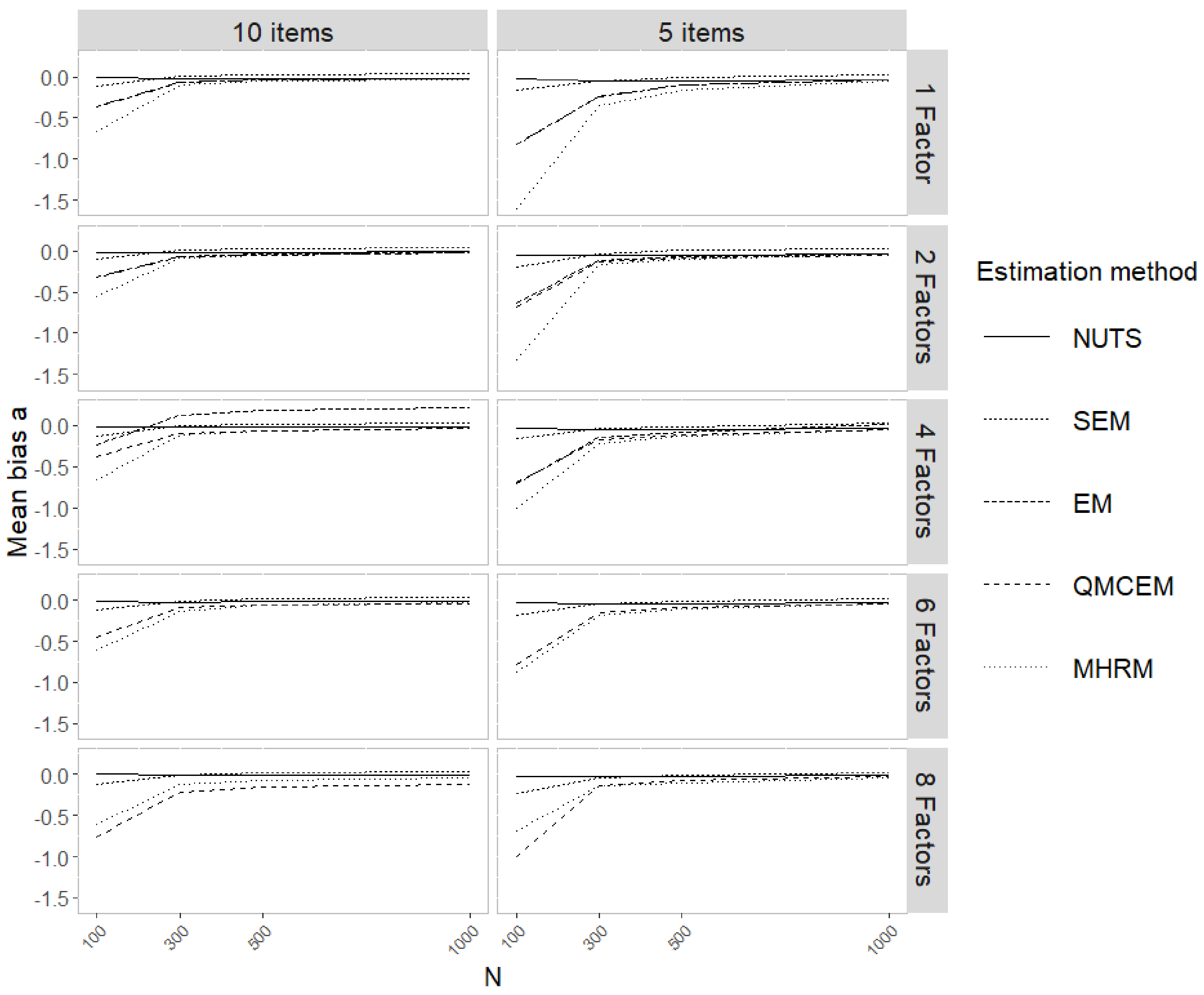
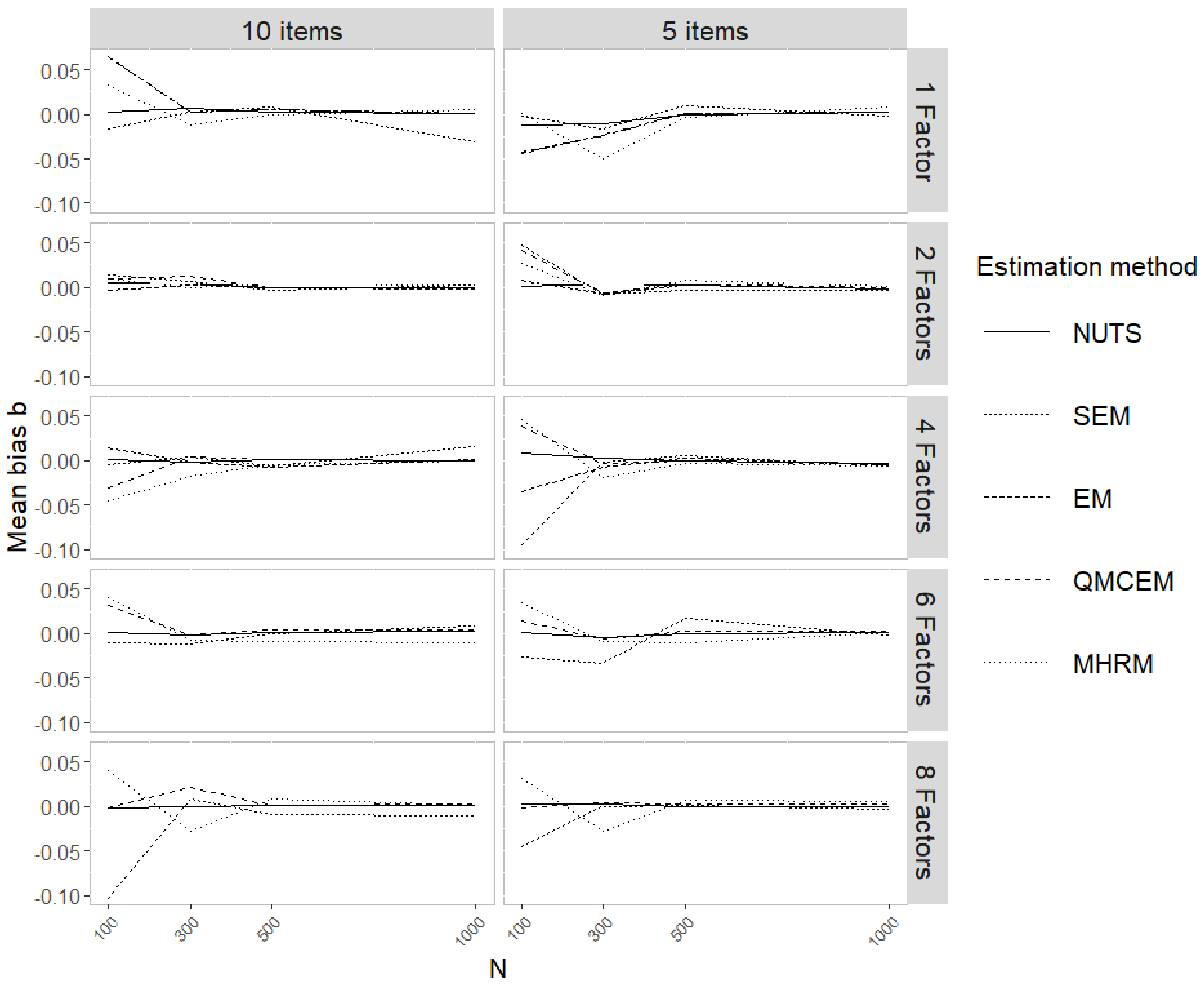
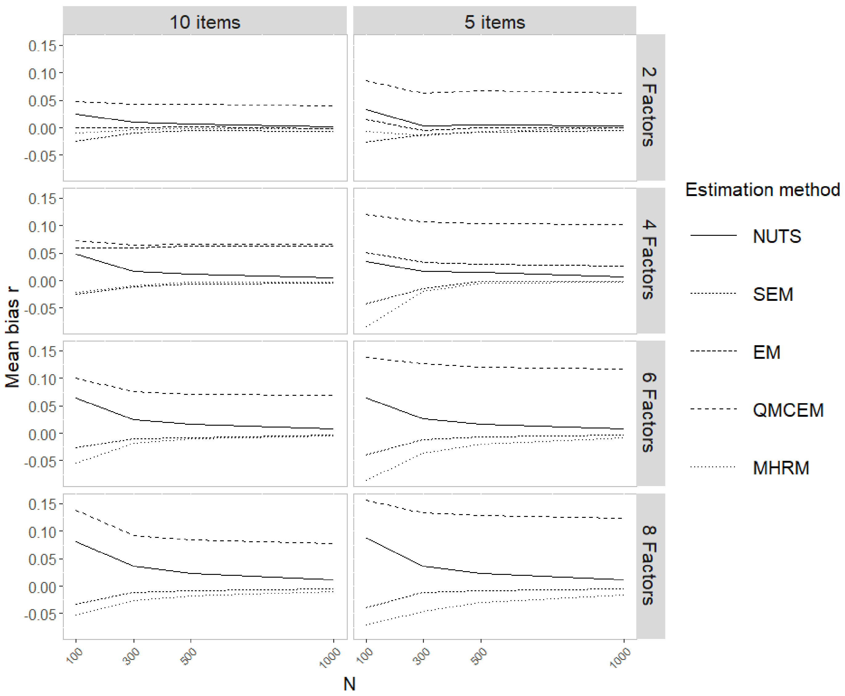
For the average bias (

Table 3. Average Bias for each method across D and N conditions.

N		100			300			500			1000
	r	a	b	r	a	b	r	a	b	r	a	b
NUTS	0.054	−0.022	<0.001	0.021	−0.032	<0.001	0.015	−0.029	<0.001	0.007	−0.019	<0.001
WLSMV	−0.030	−0.090	−0.011	−0.012	−0.013	−0.005	−0.006	0.009	0.002	−0.004	0.032	−0.003
EM	0.028	−0.283	0.004	0.021	−0.066	−0.005	0.024	−0.022	<0.001	0.022	0.018	<0.001
QMCEM	0.089	−0.291	0.009	0.088	−0.122	−0.001	0.086	−0.080	0.002	0.082	−-0.046	0.001
MHRM	−0.052	−0.274	0.023	−0.022	−0.113	−0.015	−0.012	−0.076	−0.001	−0.006	−0.037	0.001
D	1			2			4			6			8
	a	b	r	a	b	r	a	b	r	a	b	r	a	b
NUTS	−0.028	−0.001	0.011	−0.032	0.002	0.019	−0.030	0.001	0.029	−0.025	<0.001	0.039	−0.014	0.001
WLSMV	−0.015	−0.006	−0.012	−0.007	0.004	−0.011	−0.008	−0.004	−0.011	−0.007	−0.005	−0.011	−0.002	−0.009
EM	−0.112	0.001	<0.001	−0.097	−0.001	0.049	−0.012	−0.002	–	–	–	–	–	–
QMCEM	−0.112	0.001	0.055	−0.112	0.005	0.086	−0.121	0.003	0.099	−0.112	−0.001	0.112	−0.131	0.002
MHRM	−0.136	0.001	−0.008	−0.093	0.004	−0.014	−0.088	−0.011	−0.020	−0.082	−0.005	−0.026	−0.072	0.002

), for the difficulty b parameter, the differences in bias between estimation methods are small, as all of them achieved average bias of zero up to the first decimal (Figure 1). For the factor correlations r, we find that WLSMV results in the lowest bias, followed by NUTS, EM, and MHRM, consistently across conditions (Figure 2). Finally, for the discrimination a parameters, we see the largest bias differences between methods, where NUTS and WLSMV result in the lowest bias, followed by EM. While QMCEM and MHRM show the highest average bias (Figure 3). Across simulation conditions, we see that, in general, as sample size increases bias decreases. MHRM presents lower bias as number of factors increase.

When looking at absolute bias in

Table 4. Average absolute bias for each method across D and N conditions.

N		100			300			500			1000
	r	a	b	r	a	b	r	a	b	r	a	b
NUTS	0.091	0.405	0.208	0.049	0.285	0.133	0.037	0.232	0.107	0.026	0.169	0.077
WLSMV	0.099	0.597	0.576	0.050	0.344	0.231	0.037	0.265	0.151	0.026	0.189	0.103
EM	0.087	0.726	0.446	0.055	0.378	0.174	0.047	0.294	0.133	0.038	0.211	0.094
QMCEM	0.122	0.703	0.434	0.110	0.404	0.193	0.105	0.322	0.148	0.100	0.246	0.113
MHRM	0.114	0.696	0.429	0.055	0.359	0.166	0.039	0.268	0.120	0.027	0.181	0.083
D	1			2			4			6			8
	a	b	r	a	b	r	a	b	r	a	b	r	a	b
NUTS	0.276	0.132	0.047	0.277	0.131	0.048	0.273	0.131	0.051	0.270	0.131	0.056	0.266	0.131
WLSMV	0.337	0.220	0.051	0.331	0.236	0.049	0.325	0.246	0.046	0.319	0.241	0.045	0.308	0.237
EM	0.364	0.189	0.045	0.343	0.176	0.064	0.442	0.229	–	–	–	–	–	–
QMCEM	0.363	0.189	0.066	0.370	0.190	0.101	0.387	0.204	0.120	0.392	0.200	0.156	0.435	0.213
MHRM	0.373	0.176	0.045	0.326	0.160	0.046	0.302	0.150	0.047	0.286	0.150	0.047	0.265	0.137

, for the factor correlation r, most estimation methods present similar absolute bias (NUTS, WLSMV, EM, and MHRM), while QMCEM consistently presents higher absolute bias. As sample size increases, the bias decreases from around 0.09 to around 0.02. NUTS, WLSMV, and MHRM present consistent absolute bias as the number of factors increase, while QMCEM absolute bias increases as the number of factors increases.

For the difficulty b parameters, we see that NUTS results in the lowest absolute bias across N and D, while the other methods show similar absolute bias; the only exception is that MHRM presents absolute bias similar to NUTS when the number of factors is larger. As sample size increases, we see the bias decrease, and with $N=1000$ the bias for NUTS and MHRM are similar, while the other three methods stay similar across conditions.

Lastly, for the discrimination a parameter, NUTS again shows the lowest absolute bias, followed by WLSMV, and EM. QMCEM and MHRM show similar absolute bias. For all the methods, as sample size increases, bias decreases. With larger sample sizes, WLSMV and MHRM absolute bias becomes similar to NUTS, while EM and QMCEM consistently presents larger bias. As number of factors increase, MHRM presents lower bias, still NUTS presents lower bias across D (plots with the bias and the 90% CI for each method across simulation conditions are presented on the OSF site for this project: https://osf.io/9drne/, accessed on 1 August 2021).

As we simulated population parameters from continues distributions, we looked further into the bias across different ranges from the parameter values. We split the population parameters into three quantiles, presenting bias across low, medium, and high ranges. As the discrimination parameter followed the distribution $a\sim U(0.4,3)$, the low range was values lower than 1.258, medium ranged from 1.258 to 2.116, and high values were greater than 2.116. As the difficulty parameter followed the distribution $b\sim N(0,1)$, the low ranges were values lower than −0.439, the medium range was between −0.439 and 0.412, and the high values were greater than 0.412. As the the factor correlations followed the distribution $r\sim U(0.2,0.6)$, the low range were values lower than 0.332, the medium range was between 0.332 and 0.464, and high values were greater than 0.464.

The average bias across ranges of population values and sample sizes is presented in

Table 5. Average bias for each method across N and different levels of the population values.

a		100			300			500			1000
	Low	Medium	High	Low	Medium	High	Low	Medium	High	Low	Medium	High
NUTS	−0.052	−0.059	0.059	−0.007	−0.027	−0.039	−0.002	−0.020	−0.044	−0.000	−0.008	−0.032
WLSMV	−0.091	−0.114	−0.045	−0.035	−0.012	0.017	−0.026	0.008	0.049	−0.020	0.028	0.088
EM	−0.037	−0.215	−0.544	0.024	0.021	−0.068	0.028	0.053	0.019	0.033	0.076	0.116
QMCEM	−0.098	−0.281	−0.497	−0.040	−0.110	−0.230	−0.031	−0.080	−0.150	−0.025	−0.056	−0.083
MHRM	−0.075	−0.216	−0.414	−0.022	−0.074	−0.210	−0.015	−0.051	−0.140	−0.009	−0.025	−0.072
b		100			300			500			1000
	Low	Medium	High	Low	Medium	High	Low	Medium	High	Low	Medium	High
NUTS	−0.003	0.002	0.005	0.011	0.001	−0.012	0.008	0.002	−0.008	0.007	0.000	−0.005
WLSMV	0.223	0.011	−0.302	0.101	0.009	−0.115	0.071	0.002	−0.074	0.048	0.000	−0.050
EM	0.137	0.001	−0.104	0.097	0.002	−0.106	0.079	0.002	−0.087	0.068	0.001	−0.069
QMCEM	0.100	−0.004	−0.101	0.037	0.000	−0.026	0.023	0.002	−0.019	0.012	0.000	−0.008
MHRM	0.184	−0.020	−0.094	0.014	−0.010	−0.043	0.008	0.001	−0.010	0.004	0.001	−0.007
r		100			300			500			1000
	Low	Medium	High	Low	Medium	High	Low	Medium	High	Low	Medium	High
NUTS	0.056	0.074	0.085	0.027	0.030	0.033	0.018	0.020	0.021	0.010	0.010	0.011
WLSMV	−0.033	−0.037	−0.031	−0.011	−0.013	−0.010	−0.007	−0.007	−0.006	−0.004	−0.004	−0.004
EM	0.035	0.047	0.065	0.031	0.039	0.051	0.032	0.040	0.049	0.031	0.037	0.045
QMCEM	0.062	0.104	0.162	0.072	0.097	0.149	0.068	0.093	0.141	0.066	0.090	0.135
MHRM	−0.053	−0.073	−0.077	−0.021	−0.032	−0.039	−0.014	−0.019	−0.022	−0.008	−0.010	−0.012

. Similar patterns as before appeared—as sample size increases, bias decreases. With $n=100$ for the a parameter we see the IRT methods presenting higher bias at higher ranges of the population values. QMCEM and MHRM repeat this pattern as sample size increases, while EM presents similar results at larger sample sizes. WLSMV presents similar bias at different ranges of the population values, except with $N=100$, where the medium range presents higher bias. NUTS presents similar bias across the different ranges of the population values.

For the b parameters, NUTS presents similar bias across different ranges, with the medium range presenting slightly smaller bias. The other methods present a pattern, with higher bias at the low and high ranges, and smaller bias at the medium range, and these differences decrease as sample size increases. For the factor correlations, NUTS, WLSMV, EM, and MHRM presents similar bias across the different ranges, while QMCEM presents higher bias as the range goes higher.

3.1.4. Variability

When looking at the estimated parameter variability, we see in

Table 6. Variability (SD) of the estimates around the population value across D and N conditions.

N		100			300			500			1000
	r	a	b	r	a	b	r	a	b	r	a	b
NUTS	0.065	0.134	0.096	0.037	0.098	0.061	0.028	0.081	0.050	0.020	0.061	0.036
WLSMV	0.098	0.450	0.840	0.051	0.169	0.443	0.030	0.141	0.234	0.020	0.078	0.242
EM	0.095	0.740	0.755	0.056	0.277	0.138	0.045	0.185	0.122	0.037	0.136	0.050
QMCEM	0.090	0.735	0.663	0.069	0.219	0.225	0.063	0.138	0.073	0.061	0.091	0.046
MHRM	0.097	0.980	0.670	0.043	0.277	0.197	0.031	0.179	0.069	0.021	0.086	0.097
D	1			2			4			6			8
	a	b	r	a	b	r	a	b	r	a	b	r	a	b
NUTS	0.147	0.093	0.066	0.109	0.070	0.034	0.079	0.054	0.031	0.067	0.049	0.033	0.058	0.047
WLSMV	0.343	0.491	0.085	0.230	0.471	0.046	0.169	0.479	0.034	0.157	0.433	0.028	0.251	0.466
EM	0.604	0.433	0.070	0.351	0.295	0.034	0.283	0.390	–	–	–	–	–	–
QMCEM	0.600	0.433	0.065	0.363	0.315	0.059	0.326	0.324	0.062	0.376	0.342	0.086	0.551	0.323
MHRM	0.917	0.402	0.078	0.640	0.346	0.052	0.503	0.315	0.045	0.403	0.308	0.034	0.284	0.323

the standard deviation of the estimated parameter around the population values (bias). For all cases, as sample size increases, variability decreases. Across sample size, we see that NUTS presents the smallest variability. For the factor correlations, the other methods present similar variability, except that QMCEM presents higher variability at larger sample sizes. For the a parameters, WLSMV presents lower variability than the IRT methods, but this difference decreases as N increases. While for the b parameters, the IRT methods present smaller variability than WLSMV.

Across the number of factors, for the factor correlations, NUTS, WLSMV, and EM present smaller variability in most cases, as number of factors increase MHRM variability decrease, while QMCEM variability increases. For the a parameter, NUTS presents the smaller variability, followed by WLSMV. With EM and QMCEM having similar levels, MHRM variability goes from the highest in the one-factor model, to being close to WLSMV with eight factors. Lastly, for the b parameters, NUTS present the smallest variability and is consistent across the different number of factors. The IRT methods present similar levels of variability, and WLSMV presents the larger variability (plots comparing the estimation methods variability across simulation conditions are presented on the OSF site for this project: https://osf.io/9drne/, accessed on 1 August 2021).

3.1.5. Coverage

We were also interested in whether each of the methods would result in users making the correct inference—that is, that the parameters from the true population model fall within their respective 95% CI.

Table 7. Average coverage of the 95% CI for the population value across D and N conditions.

N		100			300			500			1000
	r	a	b	r	a	b	r	a	b	r	a	b
NUTS	97.6	96.0	96.1	98.3	95.4	95.6	98.7	95.1	95.3	98.8	94.8	95.2
WLSMV	93.9	90.9	95.2	97.3	92.5	95.6	98.2	92.4	95.5	98.5	91.8	95.4
EM	97.3	93.6	61.2	95.0	92.4	72.8	92.2	91.1	73.6	85.1	88.3	74.5
QMCEM	98.9	94.3	62.7	95.2	92.3	74.0	90.0	90.0	74.3	78.2	85.2	72.8
MHRM	79.7	91.8	65.6	87.9	92.1	74.3	90.0	91.7	75.4	91.2	91.2	76.3
D	1			2			4			6			8
	a	b	r	a	b	r	a	b	r	a	b	r	a	b
NUTS	95.5	95.6	99.1	95.4	95.7	98.7	95.4	95.5	98.2	95.3	95.5	97.5	95.1	95.5
WLSMV	92.1	95.6	97.2	91.8	95.4	97.4	91.9	95.4	97.4	92.0	95.4	97.4	92.1	95.4
EM	95.1	73.6	99.0	95.1	73.9	84.4	82.6	65.4	–	–	–	–	–	–
QMCEM	95.1	73.6	98.9	93.0	72.2	88.3	89.2	71.7	84.1	85.5	70.9	78.0	79.9	69.5
MHRM	94.0	74.3	97.2	95.0	74.9	92.3	92.3	74.6	85.4	89.0	74.3	78.8	86.8	73.1

shows the average percentage of times that the respective 95% CI included the population value. Overall, NUTS has the highest coverage, with an average of at least 95.1%, and as high as 99.1% across all sample sizes and number of factors. It is followed by WLSMV with an average coverage of at least 90.9% and up to 98.5% across all sample sizes and number of factors. All the IRT methods presented low coverage for the b parameter, around 62% for small sample sizes, and increases to be around 72% with larger samples. Consistently show similar coverage across different number of factors, around 70%. They show similar coverage for the a parameter, across different sample sizes presented similar results around 92%, except with large sample size QMCEM and EM presented slightly lower at 85% and 88%, respectively. Across different numbers of factors in the model, their coverage is high (around 93%) with one or two factors, but as the number of factors increases, coverage decreases down to 79.% and 86.8% for QMCEM and MHRM, respectively. For the r parameter, we see that EM and QMCEM start with high coverage with a small sample and decrease as sample sizes increases, while MHRM starts with low coverage at small sample size and increases as sample size increases. Across a different number of factors, all IRT methods have high coverage with small number of factors, and it decreases for all of them as the number of factors increases, going from being around 95% to being around 78%.

4. Discussion

In this paper, we conducted the largest between-item multidimensional IRT simulation of which we are aware, comparing popular estimation methods in terms of convergence and parameter recovery. The present projects adds to the literature about estimation methods for latent variable models with binary indicators by studying the performance of a variety of estimation methods across a large number of simulation conditions. Whereas, previous research focused on either a small number of estimation methods or a small number of simulation conditions. Further, the results present a detailed comparison across sample size and number factors in the model [6,8,9,10,11,13,33,34,35,36,37].

We found that the NUTS MCMC estimation method was the most effective, showing highest rates of convergence across conditions, and not presenting improper solutions or outliers. BMIRT models constrain the estimated parameters to be admissible values, presenting an advantage over the frequentist counterparts. While the frequentist estimation methods can lead to nonconvergence or improper solutions, this most commonly happens with small sample size and large models.

For IRT full information estimation methods, the EM algorithm works well when the models have a small number of factors (four or fewer), but failed to converge with larger models. When the model includes more factors, the best-performing method was MHRM, as it overcomes the EM limitations by using an MCMC sampling method instead of fixed quadrature points. In some cases, MHRM resulted in outlier results or was unable to compute standard errors.

The limited information method (WLSMV) showed the second-highest rate of convergence, and resulted in outliers or improper solutions (Heywood cases) in a some cases; however, the improper solutions and outliers presented more commonly across small samples and large models. WLSMV performance was not affected by either sample size of model size, indicating that when converged models do not present improper solution, it is a reliable estimation method.

The NUTS MCMC estimation method for Bayesian inference presented the best convergence rate, and when allowed to increase iterations always found a proper solution (based on the simulation conditions). This is an expected behavior based on the sampler’s ability to handle complex and large parameter spaces [30]. The use of priors allowed the model to avoid improper solutions and outliers, as they are implemented to limit the parameter space based on the model characteristics instead of sample characteristics (Equation (2)). For example, the difficulty b parameter was in the same metric as the underlying factors ($N(0,1)$), the discrimination a parameter was in the log-normal metric which is not expected to reach high values, and the factor correlations had a limited parameter space (uniform). In this way, NUTS takes advantage of this known information to facilitate estimation.

Regarding parameter bias, the NUTS method consistently presented the lowest bias across the different parameters, followed by WLSMV. The EM algorithm presented the lowest bias across IRT full information methods but failed to converge for high-dimensional models. While MHRM presented similar bias to NUTS and WLSMV for the b parameter and factor correlations, it showed higher bias for the a parameter. When looking at the inferences that would be drawn from the results of each estimation method, we find that NUTS and WLSMV have the highest CI coverage of the true population value, above 90% for all parameters. While the IRT methods present high coverage for the a and r parameters, all of them present low CI coverage for the b parameter.

Limitations and Future Research

As with any simulation study, we could not include all possible conditions to study. We focused on between-item MIRT models, but many applied studies will also be interested in within-item MIRT models. More research is needed to evaluate whether the estimation methods follow similar behavior as the ones presented in the project. Another limitation is that we focus on the comparison of the estimation methods as implemented by the mirt R package for the IRT frequentist models, the lavaan R package for the WLSMV model, and the general Bayesian program Stan for the NUTS MCMC sampler. Other IRT software can have better performing optimizers, leading to higher rates of convergence; however, we would expect the bias and overall performance to be similar across software programs.

Based on what researchers often see in practice, we evaluated the estimation method up to eight-factor models, considering this a large number of factors for applied research in general. It would be useful to extend this research to even larger models, and find what (if any) is the limit for number of factors that can be estimated with the best-behaving methods from this project (NUTS, WLSMV, and MHRM).

The present research focused on between-item compensatory multidimensional IRT models; further research is needed to evaluate the estimation methods across within-item and non-compesatory MIRT model.

5. Recommendations and Conclusions

In summary, for models with few factors (and large enough sample size), the estimation methods examined in this paper have similar performance. As the number of factors increases, the NUTS MCMC method is the most recommended to yield convergence without yielding improper results, as well as presenting consistent results across different sample sizes. Within the frequentist framework, the WLSMV method was the best-performing one, but researchers should be aware of possible Heywood cases. Among the full information IRT estimation methods, MHRM is the best-performing method, but researchers should consider limitations related to the bias of the a parameters and coverage of the b parameters. We think these results are informative, due to the increasing ease with which researchers can develop large assessments and collect large datasets.

References

1. Reckase, M.D. Multidimensional Item Response Theory, 1st ed.; Springer Publishing Company, Incorporated: Heidelberg, Germany, 2009. [Google Scholar]
2. Fox, J.P. Bayesian Item Response Modeling: Theory and Applications; Statistics for Social and Behavioral Sciences; Springer Publishing Company, Incorporated: Heidelberg, Germany, 2010. [Google Scholar]
3. Liu, Y.; Magnus, B.E.; O’Connor, H.; Thissen, D. Multidimensional Item Response Theory. In The Wiley-Blackwell Handbook of Psychometric Testing; Irwing, P., Booth, T., Hughes, D., Eds.; John Wiley & Son, Ltd: Chichester, UK, 2018; pp. 445–493. [Google Scholar]
4. Bonifay, W. Multidimensional Item Response Theory; Quantitative Applications in the Social Sciences; SAGE Publications: London, UK, 2019. [Google Scholar]
5. Adams, R.J.; Wilson, M.; Wang, W.C. The multidimensional random coefficients multinomial logit model. Appl. Psychol. Meas. 1997, 21, 1–23. [Google Scholar] [CrossRef]
6. DiStefano, C.; Morgan, G.B. A Comparison of Diagonal Weighted Least Squares Robust Estimation Techniques for Ordinal Data. Struct. Equ. Model. Multidiscip. J. 2014, 21, 425–438. [Google Scholar] [CrossRef]
7. Wirth, R.J.; Edwards, M.C. Item Factor Analysis: Current Approaches and Future Directions. Psychol. Methods 2007, 12, 58–79. [Google Scholar] [CrossRef] [PubMed] [Green Version]
8. Baker, F. An investigation of item parameter recovery characteristics of a Gibbs sampling procedure. Appl. Psychol. Meas. 1998, 22, 153–169. [Google Scholar] [CrossRef]
9. Han, K.C.T.; Paek, I. A Review of Commercial Software Packages for Multidimensional IRT Modeling. Appl. Psychol. Meas. 2014, 38, 486–498. [Google Scholar] [CrossRef]
10. Moustaki, I.; Jöreskog, K.G.; Mavridis, D. Factor Models for Ordinal Variables with Covariate Effects on the Manifest and Latent Variables: A Comparison of LISREL and IRT Approaches. Struct. Equ. Model. Multidiscip. J. 2004, 11, 487–513. [Google Scholar] [CrossRef]
11. Forero, C.G.; Maydeu-Olivares, A.; Gallardo-Pujol, D. Factor Analysis with Ordinal Indicators: A Monte Carlo Study Comparing DWLS and ULS Estimation. Struct. Equ. Model. Multidiscip. J. 2009, 16, 625–641. [Google Scholar] [CrossRef]
12. Flora, D.B.; Curran, P.J. An Empirical Evaluation of Alternative Methods of Estimation for Confirmatory Factor Analysis with Ordinal Data. Psychol. Methods 2004, 9, 466–491. [Google Scholar] [CrossRef] [Green Version]
13. Kuo, T.C.; Sheng, Y. A Comparison of Estimation Methods for a Multi-unidimensional Graded Response IRT Model. Front. Psychol. 2016, 7. [Google Scholar] [CrossRef] [Green Version]
14. Svetina, D.; Valdivia, A.; Underhill, S.; Dai, S.; Wang, X. Parameter Recovery in Multidimensional Item Response Theory Models Under Complexity and Nonnormality. Appl. Psychol. Meas. 2017, 41, 530–544. [Google Scholar] [CrossRef] [PubMed]
15. Smits, N.; Öğreden, O.; Garnier-Villarreal, M.; Terwee, C.B.; Chalmers, R.P. A study of alternative approaches to non-normal latent trait distributions in item response theory models used for health outcome measurement. Stat. Methods Med. Res. 2020. [Google Scholar] [CrossRef]
16. Bock, R.D.; Aitkin, M. Marginal maximum likelihood estimation of item parameters: Application of an EM algorithm. Psychometrika 1981, 46, 443–459. [Google Scholar] [CrossRef]
17. Jank, W. Quasi-Monte Carlo sampling to improve the efficiency of Monte Carlo EM. Comput. Stat. Data Anal. 2005, 48, 685–701. [Google Scholar] [CrossRef]
18. Wei, G.C.G.; Tanner, M.A. A Monte Carlo Implementation of the EM Algorithm and the Poor Man’s Data Augmentation Algorithms. J. Am. Stat. Assoc. 1990, 85, 699–704. [Google Scholar] [CrossRef]
19. Caflisch, R.E.; Morokoff, W.; Owen, A. Valuation of mortgage-backed securities using Brownian bridges to reduce effective dimension. J. Comput. Financ. 1997, 1, 27–46. [Google Scholar] [CrossRef]
20. Cai, L. High-dimensional Exploratory Item Factor Analysis by A Metropolis–Hastings Robbins–Monro Algorithm. Psychometrika 2010, 75, 33–57. [Google Scholar] [CrossRef] [Green Version]
21. Cai, L. Metropolis-Hastings Robbins-Monro Algorithm for Confirmatory Item Factor Analysis. J. Educ. Behav. Stat. 2010, 35, 307–335. [Google Scholar] [CrossRef]
22. Robbins, H.; Monro, S. A Stochastic Approximation Method. Ann. Math. Stat. 1951, 22, 400–407. [Google Scholar] [CrossRef]
23. Chalmers, R.P. mirt: A Multidimensional Item Response Theory Package for the R Environment. J. Stat. Softw. 2012, 48, 1–29. [Google Scholar] [CrossRef] [Green Version]
24. Bovaird, J.A.; Kozoil, N.A. Measurement models for ordered-categorical indicators. In Handbook of Structural Equation Modeling; Hoyle, R.H., Ed.; Guilford Press: New York, NY, USA, 2012; pp. 495–511. [Google Scholar]
25. Browne, M.W. Asymptotically distribution-free methods for the analysis of covariance structures. Br. J. Math. Stat. Psychol. 1984, 37, 62–83. [Google Scholar] [CrossRef]
26. Kamata, A.; Bauer, D.J. A Note on the Relation between Factor Analytic and Item Response Theory Models. Struct. Equ. Model. Multidiscip. J. 2008, 15, 136–153. [Google Scholar] [CrossRef]
27. Gelman, A.; Carlin, J.; Stern, H.; Dunson, D.; Vehtari, A.; Rubin, D. Bayesian Data Analysis, 3rd ed.; Chapman and Hall/CRC: London, UK, 2014. [Google Scholar]
28. Song, X.Y.; Lee, S.Y. Basic and Advanced Bayesian Structural Equation Modeling: With Applications in the Medical and Behavioral Sciences; Probability and Statistics; John Wiley & Son, Ltd.: West Sussex, UK, 2012. [Google Scholar]
29. Merkle, E.C.; Wang, T. Bayesian latent variable models for the analysis of experimental psychology data. Psychon. Bull. Rev. 2018, 25, 256–270. [Google Scholar] [CrossRef] [PubMed] [Green Version]
30. Hoffman, M.D.; Gelman, A. The No-U-Turn Sampler: Adaptively Setting Path Lengths in Hamiltonian Monte Carlo. J. Mach. Learn. Res. 2014, 15, 1593–1623. [Google Scholar]
31. Carpenter, B.; Gelman, A.; Hoffman, M.D.; Lee, D.; Goodrich, B.; Betancourt, M.; Brubaker, M.; Guo, J.; Li, P.; Riddell, A. Stan: A probabilistic programming language. J. Stat. Softw. 2017, 76, 1–32. [Google Scholar] [CrossRef] [Green Version]
32. Lewandowski, D.; Kurowicka, D.; Joe, H. Generating random correlation matrices based on vines and extended onion method. J. Multivar. Anal. 2009, 100, 1989–2001. [Google Scholar] [CrossRef] [Green Version]
33. Bandalos, D.L. Relative Performance of Categorical Diagonally Weighted Least Squares and Robust Maximum Likelihood Estimation. Struct. Equ. Model. Multidiscip. J. 2014, 21, 102–116. [Google Scholar] [CrossRef]
34. Kiliç, A.; Uysal, I.; Atar, B. Comparison of confirmatory factor analysis estimation methods on binary data. Int. J. Assess. Tools Educ. 2020, 451–487. [Google Scholar] [CrossRef]
35. Kiliç, A.F.; Doğan, N. Comparison of confirmatory factor analysis estimation methods on mixed-format data. Int. J. Assess. Tools Educ. 2021, 21–37. [Google Scholar] [CrossRef]
36. Natesan, P. Comparing interval estimates for small sample ordinal CFA models. Front. Psychol. 2015, 6. [Google Scholar] [CrossRef] [Green Version]
37. Asparouhov, T.; Muthen, B. Comparison of computational methods for high dimensional item factor analysis. 2012. Unpublished work. [Google Scholar]
38. R Core Team. R: A Language and Environment for Statistical Computing; R Foundation for Statistical Computing: Vienna, Austria, 2020. [Google Scholar]
39. Rosseel, Y. lavaan: An R Package for Structural Equation Modeling. J. Stat. Softw. 2012, 48, 1–36. [Google Scholar] [CrossRef] [Green Version]
40. Stan Development Team. RStan: The R Interface to Stan. 2020. R Package Version 2.21.2. Available online: https://mc-stan.org/rstan/authors.html (accessed on 1 August 2021).
41. Gelman, A.; Rubin, D. Inference from iterative simulation using multiple sequences. Stat. Sci. 1992, 7, 457–472. [Google Scholar] [CrossRef]
42. Brooks, S.; Gelman, A. General methods for monitoring convergence of iterative simulations. J. Comput. Graph. Stat. 1998, 7, 434–455. [Google Scholar] [CrossRef] [Green Version]
43. van Driel, O.P. On various causes of improper solutions in maximum likelihood factor analysis. Psychometrika 1978, 43, 225–243. [Google Scholar] [CrossRef]
44. Kolenikov, S.; Bollen, K.A. Testing Negative Error Variances: Is a Heywood Case a Symptom of Misspecification? Sociol. Methods Res. 2012, 41, 124–167. [Google Scholar] [CrossRef]
Figure 1. Average bias on the b parameter across simulation conditions, for all estimation methods.
Psych 03 00029 g001
Figure 2. Average bias on the r parameter across simulation conditions, for all estimation methods.
Psych 03 00029 g002
Figure 3. Average bias on the a parameter across simulation conditions, for all estimation methods.
Psych 03 00029 g003